BIM and BEM Methodologies Integration in Energy-Efficient Buildings Using Experimental Design

Abstract

Linking Building Information Modelling and Building Energy Modelling methodologies appear as a tool for the energy performance analysis of a dwelling, being able to build the physical model via Autodesk Revit and simulating the energy modeling with its complement Autodesk Insight. A residential two-story house was evaluated in five different locations within distinct climatic zones to reduce its electricity demand. Experimental Design is used as a methodological tool to define the possible arrangement of results emitted via Autodesk Insight that exhibits the minor electric demand, considering three variables: Lighting efficiency, Plug-Load Efficiency, and HVAC systems. The analysis concluded that while the higher the efficiency of lighting and applications, the lower the electric demand. In addition, the type of climate and thermal characteristics of the materials that conform to the building envelope have significant effects on the energetic performance. The adjustment of different energetic measures and its comparison with other climatic zones enable decision-makers to choose the best combination of variables for developing strategies to lower the electric demand towards energy-efficient buildings.

1. Introduction

Part of the energy consumption in buildings is a consequence of highly demanding appliances and utilities employed to offer comfort and accomplishing daily tasks (heating, cooling, lighting, computer devices, cooking, and others). However, some inconvenience could appear when energy demand exceeds the user’s economic and environmental parameters, including risk for traditional power grid systems [1,2].

For a better understanding of the energy performance of a building, and because energy waste must be reduced, some tools have appeared in recent years to simulate the energy demand and consumption of a dwelling. The utilization of Building Information Modelling (BIM) and Building Energy Modelling (BEM) methodologies could be a helpful tool to achieve it.

The BIM-BEM interoperability becomes necessary to incorporate energy performance analysis in the early steps of the building project. It permits the calculation of Energy Use Intensity (EUI), allocation of annual energy budgets, predict the year energy consumption, comparing HVAC systems and appliances, utility schedules, and defining energy and comfort standards. It is all for helping in the decision-making process to select competent and sustainable models towards energy-efficient buildings [3,4].

Data exchange between BIM and BEM applications is not a seamless task. Usually, it requires manual intervention and data transformation [5] due to the need for available software programs that support a robust BIM-BEM translation process. Some interoperability issues in the manual process appear because the model’s focus remains on the construction documentation rather than the energy performance simulation [6]. This situation traduces in incomplete or incorrect HVAC system modeling, missing information about controls and internal loads, and difficulties reading geometry and attributes data for the physical model [5]. This situation derives from a time-consuming process and non-optimized, less energy-conscious models.

When the BIM and BEM methodologies are incorporated in the same software, the need for the manual information exchange between different software turns null. The usage of Autodesk Revit comes up as a suitable and advantageous option for proper interoperability between the BIM and BEM methodologies, using the same software via Insight 360 and Autodesk Green Building Studio suites to estimate the whole energy performance of a building [4,7,8].

Although studies were found in the literature that used a statistical approach to analyze the performance of buildings, there were no studies that applied an experimental design to study the results of the energy performance of appliances by integrating the BIM and BEM methodologies for load reduction energy in a building.

In this article, we use BIM and BEM methodologies, experimental design, and statistical analysis to simulate facilities’ energy loads a building typology representative of houses located in tropical and subtropical areas. Experimental Design’s methodology was followed to model an equation for the simulation, which considers the building characteristics, facilities, and consumption pattern. Statistical linear regression was used to determine the significance and veracity of the results during the analysis and verification process. The solutions evaluated considered air conditioning, heating, and ventilation systems with low energy consumption, low consumption lighting, and reduced energy loads following their operating hours [9,10,11,12] and maintaining or updating the required comfort levels.

By allowing the simulation of energy performance from the integration of systems, methods, and procedures that consider the variation in the characteristics of the building and facilities, the methodology used helps designers, builders, and users assess the benefits of design alternatives and upgrades and adjustments existing buildings.

In a scenario of growing scarcity of energy sources and increased demand, this work also contributes to reducing energy consumption without compromising the needs and expectations of users regarding the building’s performance, particularly concerning comfort and well-being. Another important contribution is that the solution adopted for integrating systems, methods, and procedures can inspire professional researchers to extrapolate their benefits and potential to this field of knowledge. Finally, this work also contributes to the literature on energy efficiency in dwellings.

This paper is structured into seven sections. Section 1 introduces the matter of study. Section 2 expresses the context and current reality of the evaluation of energy consumption. Section 3 explains the materials and methods followed to evaluate energy consumption by using BIM tools. Section 4 shows the case study building to validate the proposed methods presented in Section 2. Section 5 shows the results of the creation and assessment of the physical and energy models. Section 6 enables a discussion about the results obtained and their possible reasons. Finally, Section 7 briefly explains the research was done and its possible upgrades for further works.

2. Background

Power demand is increasing daily in part due to the appliances (which includes air conditioners, heaters, lamps, fans, hairdryers, irons), reaching up to 40% of total energy demand only for residential buildings [13,14]. Energy wasting in buildings is associated with inefficient systems or appliances, old-fashioned envelopes, and space distribution, lack of control systems, and misguided consumption usage [11].

To better understand the energy performance of a building, it is necessary to study its physical model. The BIM methodology consists of the development and use of computer software to simulate the construction and operation of a building accordingly to the agreement between architects, engineers, and clients (like site development, building form, and orientation, materials, services, and systems). The product is a data-rich, object-oriented, intelligent, and parametric digital model that provides benefit and essential information for the decision-making process [3]. On the other hand, BEM methodology executes the facility’s energy performance through its simulation, using predefined criteria about the building composition and utilization [4]. At this level of the analysis, the design tools and the simulation tools appear as two categories of calculation performance. The first one allows the description of the lighting and HVAC (Humidity, Ventilation, and Air Conditioning) system’s size and operation; while the second one presents the dynamic calculations considering the whole year, assessing the indoor quality and comfort, energy demand, and payback periods, saving measures [15].

The interoperability between these two methodologies had not been managed easily. In the literature, it was found that this process is accomplished by accessing the data of the BIM model through data formats like gbXML and IFC files to exchange data between two programs (one for BIM and another for BEM) for subsequent analyses, just as the interoperability between Autodesk Revit does energy plus [16], Autodesk Revit–Design-Builder [17] or Ecotect–EnergyPlus [18]. It means that the simulation happens in an isolated, manual scheme [16,17,18]. In these terms, a knowledge gap appears in the light of accurately exporting or interpreting the exchanged data [4].

The researchers that had worked on this direct link include Yarramsetty et al. [7] who performed a study where some literature review was needed to develop the building’s BIM and energy domains; then, an energy calculation tool was applied to calculate the energy demand. Utkucu et al. [19] worked on optimizing a building by modifying its façade in Autodesk Revit, creating an energy analysis model using Autodesk Insight, revising the comfort variables, and lastly comparing them with quality designs and criteria. Deepa et al. [8] also modeled a library building in Autodesk Revit to analyze it later using Autodesk Insight. It was achieved by creating a 3D model, defining some energy settings for the building, specifying a location, and creating the energy model to estimate the energy use of the building. Sharma et al. [20] made a research study following the same methodology frameworks cited above but applied to analyze the orientation of a building and its effects on lighting systems.

The utilization of REVIT to create the physical model of the building and its suites for studying the energy performance through Energy Use Intensity (EUI) appears like a feasible choice to integrate those methodologies. Nonetheless, much research needs to be done to evaluate the accuracy of the results to determine if is possible to model the energy behavior of the building and thereby establish possible economic or environmental goals.

One metric to assess the energy loads in a building is the Energy Use Intensity (EUI). It is defined as a measure of the energy consumption’s levels relative to the building’s gross area to indicate its energy performance [21,22]. The result is the calculation of annual energy use divided by total building area (kWh/m²/year). This product is utilized to measure the dwelling energy performance, and all the simulations are based on these obtained values.

Autodesk Insight provides an effective and cohesive experience for improving building energy performance. It has a robust BIM integration that allows the visualization, interaction, and specification of building performance data earlier in the design process [23]. Autodesk Insight results permit the evaluation of energy consumption (kWh/${\mathrm{m}}^2$/year) via Energy Use Intensity (EUI). To permit the optimization of the energy model, it allows the manipulation of different options of parameters such as building orientation, window-wall ratio, window shades, window glass, types of walls and roof construction, infiltration rate, lighting, and plug-load efficiency, daylighting, and occupancy controls, HVAC systems, operations schedules, and photovoltaic panel efficiency, payback limits and coverage. This optimization occurs manually by the user and shows how to increase or decrease the energy demand of the study case when selecting different options.

Autodesk Green Building Studio is a flexible cloud-based service for energy analysis that runs building performance simulations to optimize energy efficiency. It can be done by using Vasari or REVIT conceptual mass model or a more detailed model. The energy simulation results can be viewed on the GBS website [24]. Autodesk Green Building Studio allows the analysis of the energy performance results.

The concepts of Net and Nearly Zero Energy Buildings (NZEB) had become popular to describe the synergy between renewable energy systems and low energy consumption to achieve a balanced energy budget when concluded an annual cycle [14]. For Net Zero Energy Buildings, the balance between the amount of demand (significantly reduced in comparison with typical dwellings) and consumption must be fulfilled by renewable sources in a defined period (in most cases over a year) [25,26]. In addition, they could be able to export energy to the public grid, depending on the temporal matching between generation and load and the storage possibilities. Also, the definition of Nearly Zero Energy Buildings exists, which represents the constructions with a high-energy performance. The low energy demand is generated by energy from renewable sources, produced on-site or nearby [27,28]; however, this demand is not completely covered.

As part of the energy demand, occupancy schedules and residents’ habits are important aspects of a dwelling, towards the pursuit of energy efficiency. People spend most of their time in built environments; consequently, a lot of attention must be given to studying the conditions that buildings provide and their effects on humans to satisfy their need for comfort [29,30]. This parameter is crucial to guarantee the wellness of humans inside the construction because comfort and energy demand are closely related.

Comfort, as perceived by the sense organs, could be divided into thermal, visual, auditory, olfactory, and hygienic comfort [31,32]. As comfort is sensation, it is a subjective variable, which depends on the people. Nevertheless, the parameters must be specified when designing a building attempting wellness to more people [29]. The constructive characteristics must be defined contemplating the geographic localization, the activities performed by the dwellers, and the equipment involved to attenuate the discomfort because of adverse climate conditions and activities executed, all while thinking in energy-efficient measures.

Special attention is given to climatic conditions to achieve high comfort and optimum energy performance. The climate plays an important role in energy consumption and energy-efficiency systems in buildings [27]. The buildings are subjected to climate conditions which can affect the energy consumption of the building [33]. Architectural features distinguish buildings in the different climatic zones worldwide. For example, buildings in warm zones globally, such as tropical areas, are frequently designed to heighten the interactions between indoor and outdoor climates. The opposed situation occurs to constructions in cold zones, where the design tries to insulate the building from temperature exchange [27].

Through bioclimatic design and the use of design measures, a higher level of building energy efficiency and indoor thermal comfort can be achieved; the measures related to windows performance to increase ventilation levels and lighting, installation of shading devices, consideration of thermal insulation techniques, and airtightness [34,35]. The house’s orientation affects the quantity of energy to be demanded due to the linkage between environmental factors and indoor comfort. The more benefit from the orientation of the house (daylighting, shading, direction of winds), the more comfort to be felt by the occupants. The successful application of architectural features based on the climatic conditions will define and valorize the energy efficiency, exploiting the benefits that the environment offers [36], resulting in a diminution in the energy load.

Houses in tropical and sub-tropical high-income neighborhoods present elevated levels of energy consumption [37]. Most of the recent studies have highlighted the energy consumption in low-income households, and not that much in the ones in high-income dwellings; however, a few pieces of research were found, like the ones of Malama et al., Allen et al., Xu, and Williams et al. [37,38,39,40]. Apart from the design and location of the building [41,42], it was found that some of the reasons causing elevated energy consumption in bulky households are due to income and behavior of the users, age, activities developed, and the technology level of the appliances connected. The consciousness of the dwellers is another factor; high-income consumers tend to be more environmentally responsible, but it may not be applied in the personal energy-use ambit [39].

So, it could be said that high-income households, despite presenting some advantageous architectural features, appropriated for warm climates, most of them are not properly utilized, as a consequence of inadequate occupancy schedules and exacerbated utilization of electrical devices to achieve thermal comfort.

In this research, some statistical techniques to execute and validate the research methodology are required. Experimental design (or Design of Experiments) is a collection of tools used for studying the behavior of a system, involving planning and performance of experiments where a simultaneous change of many factors is carried out systematically to determine the effects of experimental variables [43,44].

It aims to systematically select or plan experiments to achieve the desired outcomes by considering the knowledge about the physical processes in the decision-making process [45]. This process is based on the analysis of how the input factors (input variables) are related to the outputs (response variables) [46].

The two main applications of experimental design are screening, in which the factors that influence the experiments are identified, and optimization, in which the optimal settings or conditions for an experiment are found. The domains that experimental design has impacted significantly comprise real experiments, simulation-based experimental design, and parameter learning or hyper-parameter tuning [47,48]. It can be achieved by balancing several features, including power, generalizability, forms of validity, practicality, and cost [49].

The manipulation of variables brings an interesting approach to its results. The effects and statistical significance of a larger group of experimental variables can be determined through factorial or screening designs, which enable choosing the relevant variables or conditions for the next set of experiments, considering different levels for each factor [12,43]. The main goal of the analysis of variance (ANOVA) is to study the total dispersion observed in the resulting values of the selected characteristics and attribute it to the examined factors that derive their significance over the system analyzed [44]. The linear regression is the equation that assumes the linear relationship between the input variables (independent variables) and the single output variable (response variable) [46].

There are many examples of experimental designs in the construction industry. Kioupis [44] handled a parametric experimental design to identify the settings of the process factors that optimize the quality characteristics of geopolymeric products. Yong et al. [50] adopted the experimental design to find optimal building envelope parameter values to minimize the heating load in a single-family house. Bustami et al. [51] investigated the potential of native plants growing in vertical walls for green buildings in Australia, considering different plant species, soil substrates, and irrigation regimes. Serbouti et al. [52] employed an experimental design to optimize a building’s energy performance in Morocco using Python and TRNSYS. Najjar et al. [12] developed research where various performance parameters related to the building design (construction materials, window-wall ratios) were analyzed to obtain the be-suited arrangement of factors that present a more efficient energy consumption for the case of study building.

However, an experimental design had not been applied to analyze the result of the interoperability between BIM and BEM methodologies statistically when studying house facilities. In this case, the approach exposed permits the evaluation of the factors (home appliances) that most affect the energy loads in the case of the study presented.

3. Materials and Methods

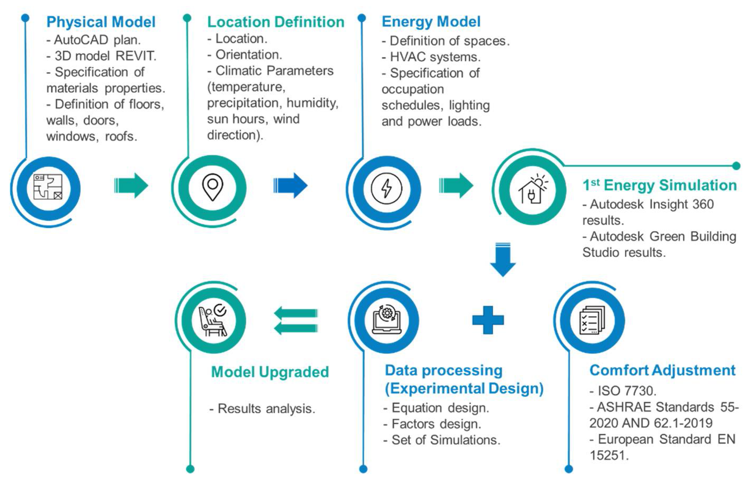
The proposed method starts with a physical model (applying the BIM methodology), then an energy model based on this physical model, and to conclude an energy simulation, it all was made to show the performance of the dwelling, as presented in Figure 1. The procedure for the realization of this research was divided into seven steps: design of the physical model, location definition, creation of energy model, development of first energy simulation, comfort adjustment following current standards, data processing using Experimental Planning, and development of statistical analysis of the model upgraded to check results.

A house whose characteristics and consumption pattern are representative of tropical and subtropical areas, with a high standard, was selected to develop this research. The house has traces that are inspired by Spanish and Italian architecture, show stucco or plaster exterior and red clay roof tiles, ornate archways, ceramic tiles on the floor, and exposed columns and beams [30]. The reason to choose this house was to analyze the possible energy performance advantages present in houses with spacious rooms, which present some attributes such as large windows, open spaces, balconies, high ceilings, shading devices, clay roofs tiles, and clear colors. These characteristics could significantly improve indoor comfort conditions by keeping a refreshed and pleasant environment inside the house [53,54].

Bulky houses similar to the one used in this study are often used in warm climates, mainly in middle/upper-class neighborhoods. This house typology has also become attractive to this whole, for having high energy loads due to its inhabitants’ behavior and weather conditions, and for having the potential to reduce energy loads and increase energy efficiency.

Performing the energy simulation requires defining the physical model. It starts with an AutoCAD plan illustrating the specifications of the construction project. Autodesk REVIT is applied later to simulate the 3D elements, such as floors, walls, doors, windows, and roofs. Furniture elements could be added using online libraries like bimobject.com [55] and revitcity.com [56] to create a more realistic physical model. Autodesk REVIT has its own materials properties, which are globally accepted. Still, for creating a realistic model, thermal properties were modified for the materials brick, concrete, travertine, and tiles based on the experimental research of Castro Ferreira [57], to perform a model with accurate real behavior following Brazilian materials.

Location Definition permits comparing the different thermal behavior in several cities and countries. In this work, five different locations for the same case study are proposed to represent the energy demand, the required comfort standards, and its relation with the climatic conditions from those locations. The five locations carefully chosen were Armação dos Búzios, in southwest Brazil; Capri, in the Mediterranean Italian coast; Punta Cana, in the Caribbean Sea; Dubai, in the Persian Gulf; and Sydney, in the East Coast of Australia; they were defined to evaluate the energy performance of the house in five different climates. It was also given an orientation of 315° to true north to the same model in the different locations. This value coincides with all locations as the most profitable one to better use climatic conditions, such as solar radiation and wind direction. In addition to these, other climatic parameters were evaluated, such as temperature, humidity, precipitation, and Sun hours, to better understand the different conditions on the energy performance of the case of study.

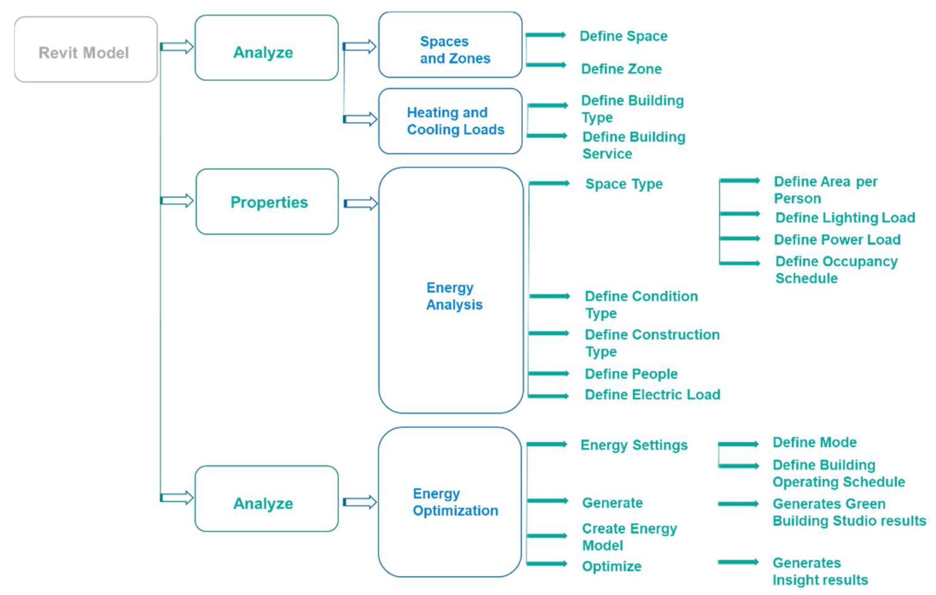
The integration between BIM and BEM methodologies is based on the definition of spaces and energy attributes. This interoperability based on REVIT is graphically explained in a flowchart in Figure 2.

The energy model was designed by defining spaces in the plans of the Revit 3D model. It was possible due to the Revit tools for separating the different spaces of the construction project to characterize them in terms of indoor comfort better. Only thermal and visual variables will be considered, such as temperature, humidity, air velocity, airflow, and illuminance, to guarantee comfort inside the house of the case of study. It is because those are the ones that can be analyzed in the physical and energy models recreated in the simulation.

The next step was grouping different spaces to create zones. These zones could permit the assignation of different HVAC systems, but in this case, was selected the same HVAC system (VAV, Hot Water Heater, Chiller 5.96 Coefficient of Performance, Boilers 84.5 efficiency) for the two zones created.

The occupation schedules, occupancy, lighting, and power loads values were defined as the “By Space Type” option suggested by default in Autodesk REVIT. These parameters were defined on purpose to perform the first energy simulation and show how the not definition of these variables could affect the energy performance; then, the correct parameters of “Energy Settings” were defined to perform the models. The energy simulations continued by clicking the “Create Energy Model” in Revit to create a 3D view of the energy model and examine no mistakes or errors [58]. In this work, five different energy simulations were carried out initially, one for each postulated city. These energy simulations were launched by clicking the “Generate” button to generate the results in the Autodesk Green Building Studio suite; and lastly, press the “Optimize” option to generate the possible optimization options in the Autodesk Insight suite.

Once the models were created and corroborated that the EUI value was elevated, two options to diminish the energy demand in the house were conceived. The first one was to adjust the available comfort values to modify within Revit (air temperature, humidity, air velocity, airflow, and air changes). The second one was to manipulate the results emitted by Autodesk Insight by lessening the significant values following real possibilities (limits established by Autodesk Green Building Studio) and leaving unchanged the options that did not offer a significant diminution of EUI.

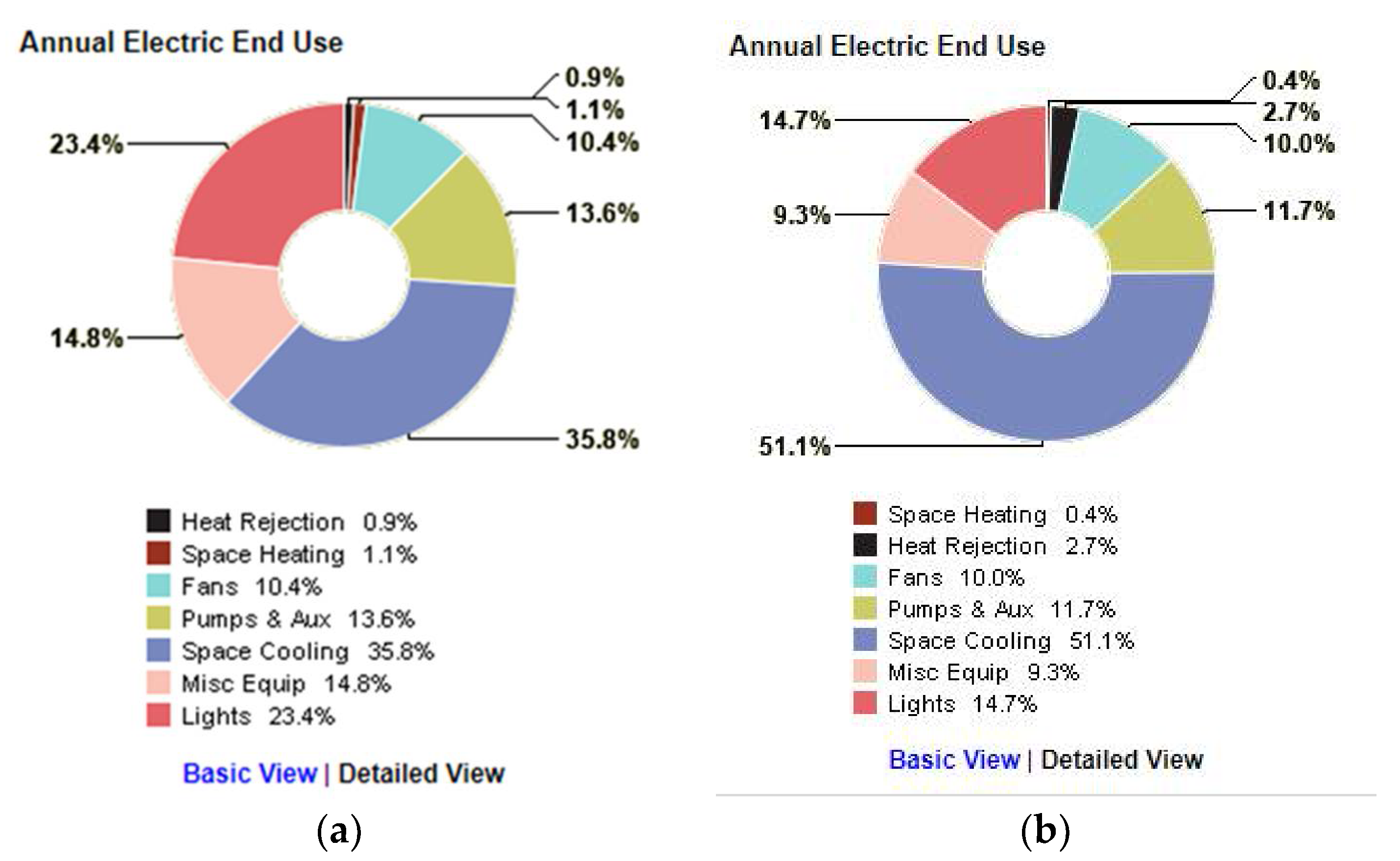
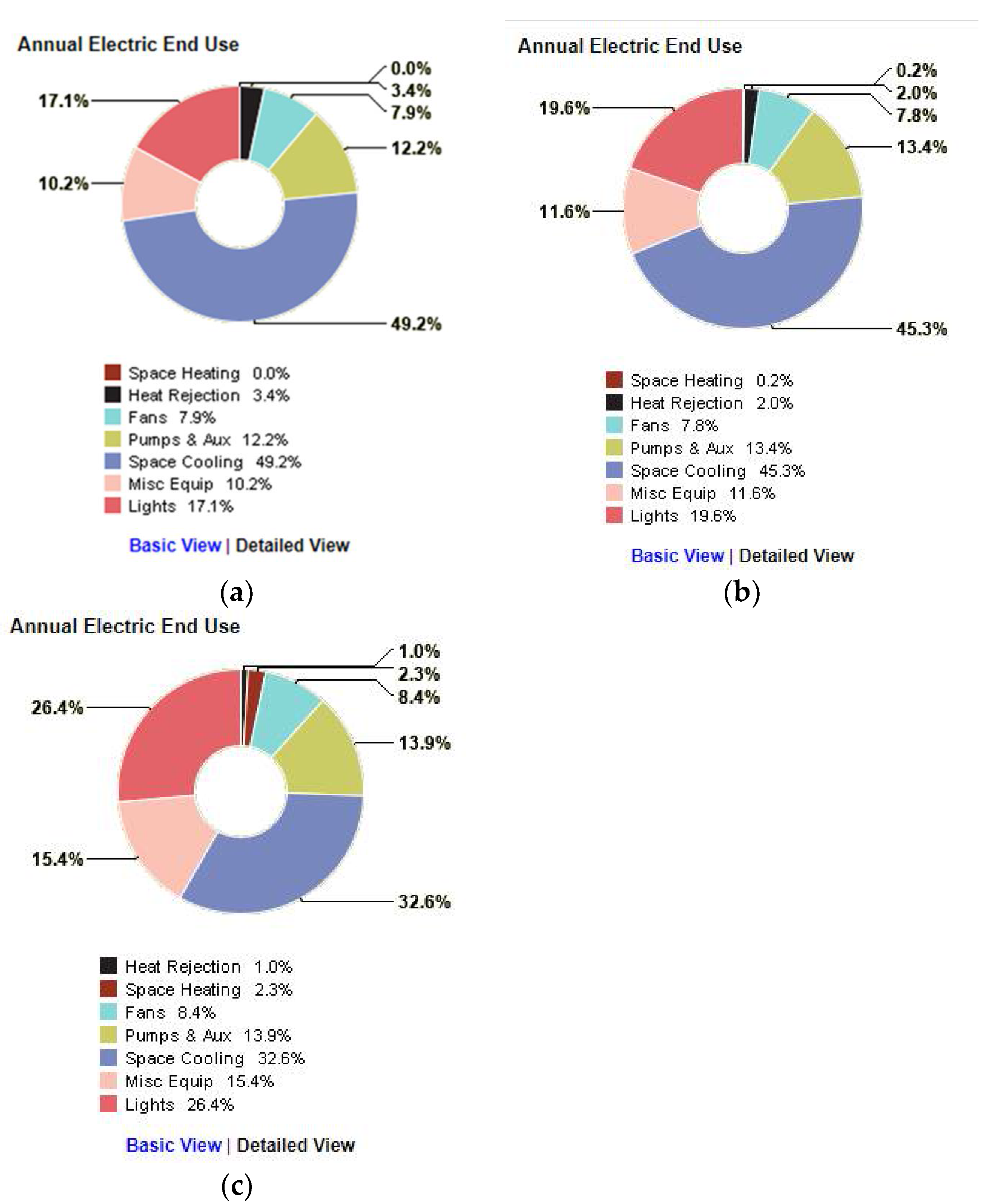
For this research work, it was considered only the Green Building Studio’s results about EUI, electric and fuel demand, photovoltaic potential (panel type, energy savings, nominal rated power, total panel area, maximum payback period), energy end-use charts, and the weather station information for every model created, to assist in the pursuit of energy-efficient or NZEB models.

The optimal comfort values were disposed of following a series of international norms and standards (ISO [59], ASHRAE [60,61], and European Standard [62], whose statutes were valid for the five constructed models. Then, they were successfully modified in the physical model.

Manipulating the different values of EUI emitted by Insight demands the use of experimental design because it is not known which combination of options may ensure a correct diminution of the energy demand. It was created an equation that could calculate the energy consumed by putting the appliances under interaction to determine its influence and possible performance solutions. The variables of the equation are called “design factors”, and their different options are called “levels”. Following the experimental design methodology, there were considered three factors (low-consumption lighting, low-consumption power loads, and HVAC systems with low energy demand); and within them, the levels were specified as three different values for lighting efficiency, two different values of load efficiency, and seven different options for the HVAC system for developing the experimental planning study. At the same time, the rest of the options to diminish the EUI emitted by Autodesk Insight were established in the minimum demand for energy.

Forty-two simulations were carried to obtain the results of the different energy performances for the different cities. The significance of the results was validated by performing a statistical linear regression, considering the p-values minor than 0.05. Once the simulations were done, it was possible to recognize in which cities and under what conditions (set of combinations) the major and minor values of EUI were achieved.

4. Case Study: Validating the Flowchart of the Methodology

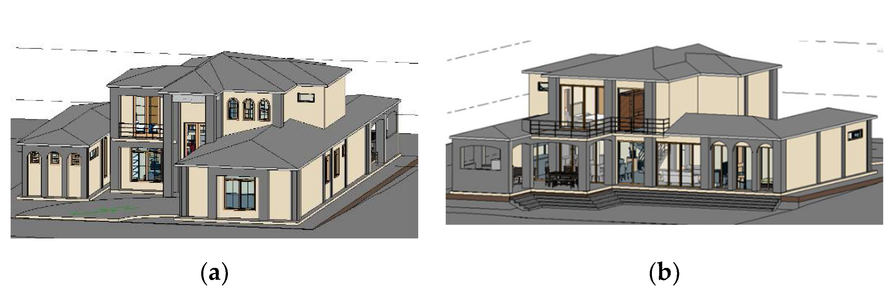
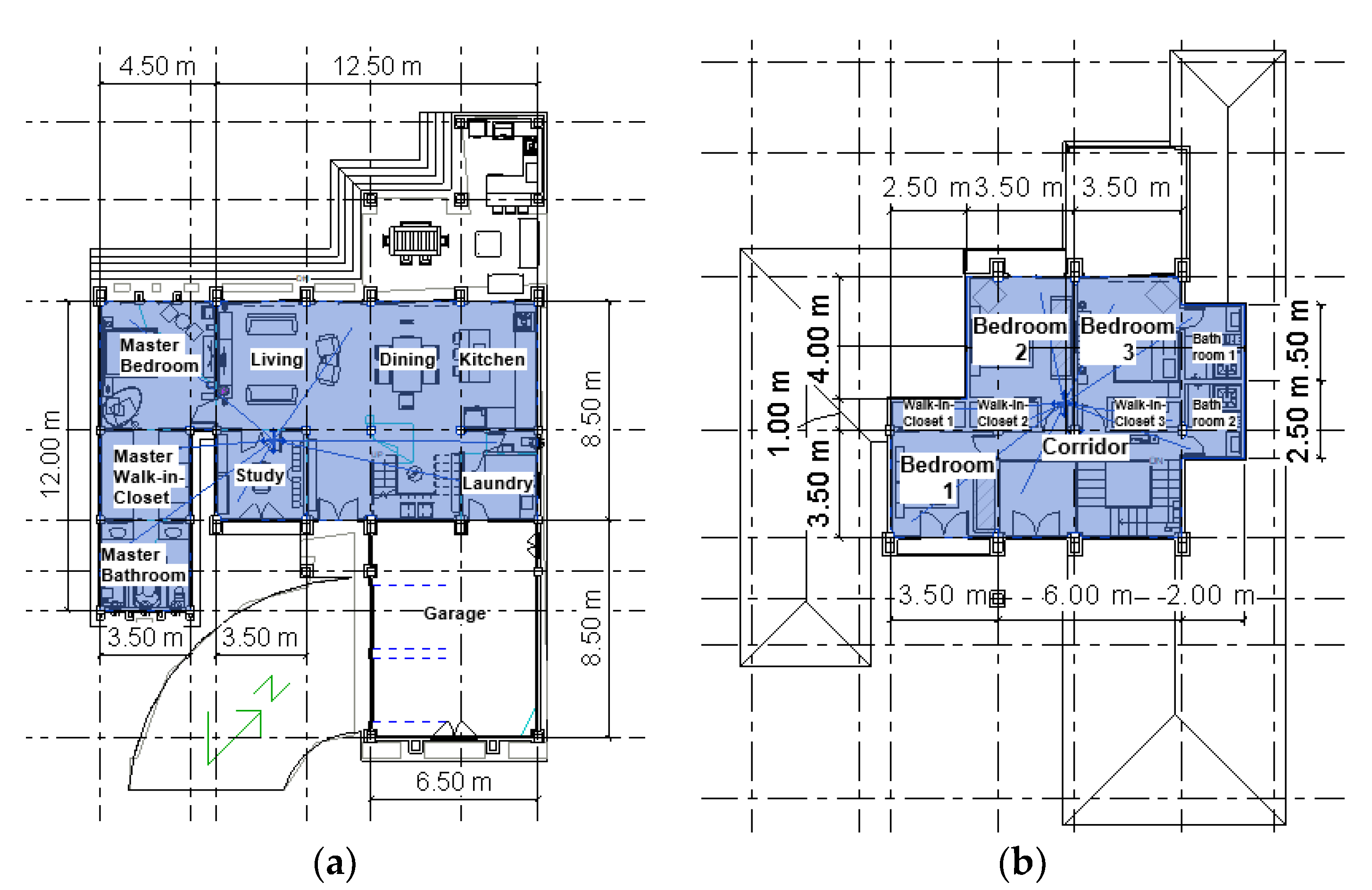
As mentioned, it was selected as a hypothetical two-story single-family house, to analyze its energy performance, particularly in zones where it is possible to find these houses (the range of the globe presenting warm climates). Figure 3 illustrates the views of the house.

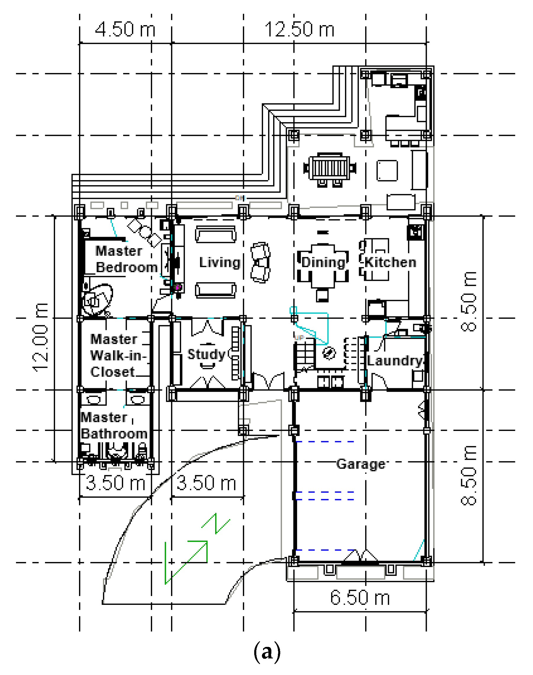
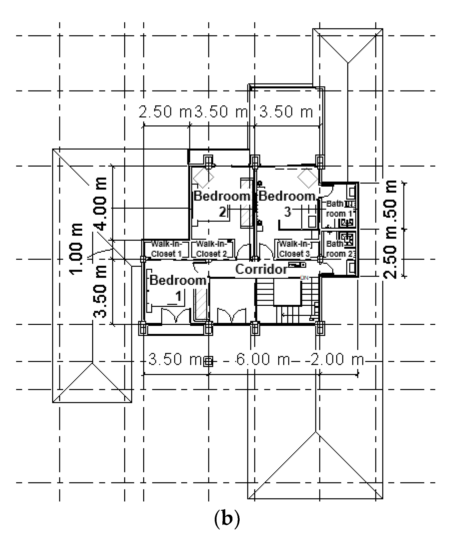
The house has an area of 250 ${\mathrm{m}}^2$ distributed in two stories. The first floor has 3 m height, and the second floor varies between 3 m and 4.42 m on its maximum height. It is composed on the lower level by a double-height entry hall, living-dining-kitchen spaces conforming a spacious room, a library, master bedroom, walk-in closet and bathroom, laundry, and a visitors ½ bathroom. Back in the hall and rising the stairs can be found three bedrooms, three walk-in closets, two bathrooms, and a balcony on the upper level. In addition, a two-car garage is integrated into the façade on the first floor, and on the backside can be found an outdoor kitchen in the covered lanai. The floor plans of the house can be seen in Figure 4. The thermal variables of the constitutive materials, which directly affect the house’s energy performance, are exhibited in

Table 1. Thermal variables of selected materials.

Material	Thermal $\mathbf{Conductivity},\mathsf{\lambda }(\mathbf{W}/\mathbf{m}·\mathbf{K})$	$\mathbf{Specific}\mathbf{Heat},\mathbf{C}(\mathbf{J}/\mathbf{g}\mathbf{·}\mathbf{°}\mathbf{C})$	$\mathbf{Density},\mathsf{\rho }(\mathbf{k}\mathbf{g}/{\mathbf{m}}^3)$	Emissivity, ε
Brick	0.90	0.92	1600	0.95
Concrete, cast-in-place	1.15	1.00	2000	0.95
Travertine	2.90	0.84	2750	0.95
Clay-roof Tiles	0.80	0.80	1900	0.90

and come directly from the study made by Castro Ferreira in Brazil [57].

It should be noticed that the thermal variables of the imported elements (furniture, doors) come directly from the online library and are unmodifiable or seen; also, thermal variables of paint are not considered due to their minimum thickness. Furthermore, thermal variables of the complete building’s elements are also considered, as can be seen in

Table 2. Thermal variables of building’s elements.

Element	Thickness (cm)	$\mathbf{Heat}\mathbf{Transfer}\mathbf{Coefficient},\mathbf{U}(\mathbf{W}/{\mathbf{m}}^2·\mathbf{K})$	Thermal $\mathbf{Resistance},\mathbf{R}({\mathbf{m}}^2·\mathbf{K}/\mathbf{W})$	Thermal Mass $(\mathbf{k}\mathbf{J}/\mathbf{K})$	Solar Heat Gain Coefficient
Wall type 1	15	6.85	0.15	22.11	-
Wall type 2	10	9.93	0.10	13.97	-
Floor	15	8.40	0.12	28.26	-
Roof	12	9.03	0.11	21.40	-
Windows	0.4	3.69	0.27	-	0.78

.

This house is north-west oriented, specifically 315 to true north. It permits a considerable entrance of daylighting, which helps with natural illuminance and warm indoor temperatures. Such an orientation is assisted by the shading elements and does not allow excessive solar radiation inside the house.

As particular features of this household, windows and doors have a significant effect on natural lighting and ventilation rates, which influences the energy demand for the appliances. The description of its characteristics can be seen in

Table 3. Doors and Windows.

Element	Quantity	Space	Material	Height (m)	Width (m)
Window 1	1	Master bathroom	Sash and Glass	0.5	2.0
Window 2	3		Wood and Glass	0.6	0.465
Sliding Door	1		Wood	2.1	1.0
Window	2	Master walk-in-closet	Wood and Glass	2.0	0.5
Sliding Door	1		Wood	2.1	1.0
Sliding Door	3	Master bedroom	Sash and Glass	2.5	1.1
Door	1		Wood	2.1	0.9
Window	1	Library	Wood and Glass	2.0	1.8
Door	1		Wood and Glass	2.5	1.6
Door	1	Entry hall	Wood and Glass	4.0	1.6
Sliding Door 1	1	Living room	Sash and Glass	2.5	2.9
Sliding Door 2	1		Sash and Glass	2.5	1.9
Sliding Door	1	Dining room	Sash and Glass	2.5	2.9
Sliding Door	1	Kitchen	Sash and Glass	2.5	1.9
Window	1	Visitors’ bathroom	Wood and Glass	0.6	0.465
Door	1		Wood	2.1	0.7
Window	1	Laundry	Wood and Glass	1.5	1.0
Door	1		Wood	2.1	0.8
Window 1	1	Garage	Wood and Glass	1.5	1.0
Window 2	1		Wood and Glass	2.0	1.8
Door 1	1		Wood	2.1	0.8
Door 2	2		Wood	2.5	2.5
Window	3	Stairs	Wood and Glass	1.2	0.6
Door 1	1	Bedroom 1	Wood and Glass	2.5	1.6
Door 2	1		Wood	2.1	0.8
Door	1	Walk-in-Closet 1	Wood	2.1	0.7
Sliding Door	1	Bedroom 2	Sash and Glass	2.5	1.83
Door			Wood	2.1	0.8
Door	1	Walk-in-Closet 2	Wood	2.1	0.7
Sliding Door	1	Bedroom 3	Sash and Glass	2.5	2.9
Door			Wood	2.1	0.8
Door	1	Walk-in-Closet 3	Wood	2.1	0.7
Window	1	Bathroom 1	Sash and Glass	0.5	1.0
Door	1		Wood	2.1	0.7
Window	1	Bathroom 2	Sash and Glass	0.5	1.0
Door	1		Wood	2.1	0.7

.

The next energy settings were defined following alternatives offered inside Autodesk Revit. The Building Type was defined as a “Single Family” house. The energy analytical model was simulated contemplating “Conceptual Masses and Building Elements”. The HVAC system selected to cool and heat the house was “VAV-Single Duct” (Central VAV, HW Heat, Chiller 5.96 COP, Boilers 84.5 eff.), provided by the Heating and Cooling loads services. For the HVAC system, were specified 17 rooms, according to the indoor spaces to define two HVAC zones, as can be seen in Figure 5. Furthermore, the location of the total rooms and zones of the case study building is illustrated in

Table 4. Rooms and zones.

Space	Room	Zone
Master bathroom	1
Master walk-in-closet	2
Master bedroom	3
Library	4
Entry hall
Living room		1
Dining room	5
Kitchen
Stairs
Visitors’ bathroom	6
Laundry	7
Garage	8	-
Bedroom 1	9
Walk-in-closet 1	10
Bedroom 2	11
Walk-in-closet 2	12
Bedroom 3	13	2
Walk-in-closet 3	14
Bathroom 1	15
Bathroom 2	16
Corridor	17

.

Every room was considered “By Space Type” (dormitory bedroom, laundry, restroom, and so on), properly defined following every space aforementioned. It means that Autodesk Revit will automatically consider the values corresponding to Area per Person (dwellers), Lighting Load Density, Power Load Density, Sensible Heat Gain per Person and Latent Heat Gain per Person by the space type selected. In addition, it was contemplated the schedules for occupancy, also “By Space Type”.

Table 5. Space type description.

Space Type	$\mathbf{Area}\mathbf{per}\mathbf{Person}({\mathbf{m}}^2)$	$\mathbf{Lighting}\mathbf{Load}\mathbf{Density}(\mathbf{W}/{\mathbf{m}}^2)$	$\mathbf{Power}\mathbf{Load}\mathbf{Density}(\mathbf{W}/{\mathbf{m}}^2)$	Sensible Heat Gain per Person (W)	Latent Heat Gain per Person (W)	Occupancy
Dormitory Bedroom	10	11.95	5.81	73.27	45.43	Home Occupancy (24 h)
Restroom	10	9.69	3.23	73.27	58.61	Home Occupancy (24 h)
Library-Audiovisual	4	13.99	16.15	73.27	58.61	Retail Facility Occupancy (7 a.m. to 8 p.m.)
Dining Area	1.5	9.69	5.81	80.56	58.61	Home Occupancy (24 h)
Laundry–Ironing and Sorting	5	6.3	32.29	80.59	139.21	Retail Facility Occupancy (7 a.m. to 8 p.m.)
Stairway	10	6.46	3.23	73.27	58.61	Home Occupancy (24 h)
Parking Area	20	2.05	3.23	73.27	58.61	Home Occupancy (24 h)

shows the space types with the respective values and schedules for its variables.

4.1. Comfort Conditions

According to ASHRAE Standard 55-2020 [59,60], which defines the thermal environmental conditions for human occupancy, the air temperature must be between 22.5 °C to 26 °C for summer (at clothing insulation factor 0.5); and between 20 °C to 23.5 °C for winter (at clothing insulation factor 0.9). Also, Standard ISO 7730 [59] suggests air temperature should be between 20 °C and 24 °C in winter and between 23 °C and 26 °C in summer.

For humidity, Standard 55-2020 also specifies between 55% and 60% during summer and an interval of 20% to 30% during winter. Likewise, ISO 7730 recommends humidity levels between 30% and 70% over the year [59]. Although Air Velocity depends significantly on the air temperature and humidity levels, for the suggested comfort values specified before, some acceptable intervals of Air Velocity are around 0 and 0.8 m/s in summer, and lesser than 0.15 m/s in winter, accordingly to ASHRAE Standard 55. For ISO 7730, at 23 °C, the optimal air velocity is 0.2 m/s. Likewise, the European Standard EN 15,251 recommends an air velocity between 0.2 and 0.8 m/s [62]. Ventilation requisites were established by ASHRAE Standard 62.1-2019 [60], suggesting a minimum of 0.3 L/S·m² of airflow, and between 0.35 and 1 air change per hour. Again, the European Standard establishes a ventilation rate of around 0.49 $\mathrm{L}/\mathrm{s}·{\mathrm{m}}^2$ and 0.7 air changes per hour [62].

The standards mentioned above were utilized to define the comfort variables of the case study, considering international terms, with the purpose to fulfill common requirements for the different locations selected worldwide and not only to accomplish regional comfort exigencies. However, the house of the case study was defined the following values in

Table 6. Comfort values considered.

	Air Temperature (°C)	Humidity (%)	Air Velocity (m/s)	$\mathbf{Air}\mathbf{Flow}(\mathbf{L}/\mathbf{s}·{\mathbf{m}}^2)$	Air Changes (ren/h)
Comfort Values	23	55	0.2	0.5	0.7

, aiming to satisfy the requirements for both winter and summer, and is following the highest number of standards possible.

4.2. Climatic Conditions

For the analysis, five locations were selected to represent five different climatic conditions and evaluate how the house’s response follows the same physical and energetic adjustments. It was used the Köppen-Geiger climate classification system. The locations were Armação dos Búzios, Rio de Janeiro state-Brazil, with Tropical Savanna climate; Capri Island, Campania region–Italia, presenting a Mediterranean Hot Summer climate; Punta Cana, La Altagracia province–Dominican Republic, exhibiting a Tropical Monsoon climate; Dubai–Dubai–United Arab Emirates, with Hot Desert climate; and Sydney, New South Wales state, manifesting a Humid Sub-Tropical climate. The reason for selecting those five locations was the possibility of encountering bulky houses similar to the one used in this study, typical of high-income neighborhoods in warm regions. Those warm regions were proposed in latitudes between the 45° north and 45° south, to include the northernmost reference, Mediterranean Sea, and the southernmost reference, the east coast of Australia.

Table 7. Climatic conditions for selected locations.

Location	Climate Type	Average High Temp (°C)	Average Low Temp (°C)	Annual Precipitation (mm)	Average Relative Humidity (%)	Sunshine Hours
Armação dos Búzios [63]	Aw	25.7	21.8	1012	81.7	3113.7
Capri [64]	Cs	18.7	16.9	938	73.6	3452.5
Punta Cana [65]	Am	29.3	23.2	1102.6	82.4	3046.3
Dubai [66]	BWh	33.2	20.1	94.7	51.8	3570.0
Sydney [67]	Cfa	21.5	15.0	912	69.3	3115.4

shows the year-average climate variables for the different locations selected for the study.

4.3. Experimental Design

The experimental design applied can be summarized by the following steps: First, the goal’s definition, which implies the possible energy reduction according to the suggestion items emitted by Autodesk Insight’s results. Second, the determination of which results to take into account to manipulate and carry on the simulations. Third, were defined the factors and levels that affected the EUI and created the equation that represents the energy consumption. Fourth, were developed the forty-two simulations that combine the different factors and levels defined above. Fifth, the different results were analyzed and determined the behavior of the EUI in the different cities following the combination of factors and levels. And lastly, it was conducted statistical analysis (analysis of variance and linear regression) to verify the accuracy of the study and determine the significance of the results obtained (the software Minitab was adopted for this calculation to conduct the main effects plot by integrating the statistical process.

4.4. Inventory of Database

Depending on the location of a house building, more or less energy will be demanded for the lighting and power loads, as much as for the HVAC systems to offer more indoor comfort conditions. To decrease the energy consumption in the house by manipulating the load of the appliance, it was idealized to alter the variables “Lighting Efficiency”, “Plug Load Efficiency” and “HVAC System” for the definition of the factors that will have a part in the execution of the experimental design process.

Lighting Efficiency ($E_L$) shows the average internal heat gain and power consumption of electric lighting per unit floor area. It consists of three levels that are offered by Autodesk Insight analysis, which are 11.95 W/m², 7.53 W/m², and 3.23 W/m², depending on the dwelling’s electric potency in lighting devices. Plug Load Efficiency ($E_P$) displays the power used by equipment in the building, such as computers, printers, washing machines, refrigerators, hairdryers, internet modems, etc. It consists of two levels, also available in the Autodesk Insight analysis which are 10.76 W/m² and 6.46 W/m², following the mentioned equipment’s load. HVAC System ($E_H$) illustrates the efficiency options range of the HVAC systems. It consists of seven levels: the different possible options, like Central VAV, ASHRAE Package System, High-Efficiency Heat Pump, High-Efficiency Package System, High-Efficiency Package Terminal AC, High-Efficiency Package VAV, and ASHRAE Package Terminal Heat Pump.

Describing the HVAC systems, the Central VAV presents a static pressure duct system with variable speed drive, a Coefficient of Performance of 5.96, and a water heater. The ASHRAE Package System has an Energy-Efficiency Ratio of 11, presenting the minimum efficiency of the HVAC systems in REVIT. The High-Efficiency Heat Pump has a Seasonal Energy-Efficiency Ratio of 17.4 and works with a constant volume cycling fan. The High-Efficiency Package System presents a small unit in a single zone system and has a Seasonal Energy-Efficiency Ratio of 20. The High-Efficiency Package Terminal AC is a type of self-contained heating and air-conditioning system, with an Energy-Efficiency Ratio of 12.7. The High-Efficiency VAV is an air terminal with a high-efficiency turndown on an air system, underflow air distribution with a Coefficient of Performance of 7.5. The Package Terminal Heat Pump consists of a separate, un-cased refrigeration system installed in a cabinet, which uses reverse cycle refrigeration as its prime heat source and has an Energy-Efficiency Ratio of 11.9.

The different levels of the factors mentioned above represent the options suggested by Autodesk Insight to dwindle the energy consumed when handling the appliance’s load in the operational phase of the case study. They were selected for being the options that offer minor electric consumption for each variable compared to the initial model generated. The factors and the levels can be shown in

Table 8. The sequence of combinations of Design Factors and Levels.

Sequence	Lighting Efficiency (W/m2)	Plug Load Efficiency (W/m2)	HVAC System
1	11.95	10.76	Central VAV, HW Heat, Chiller 5.96 COP
2	11.95	10.76	ASHRAE Package System
3	11.95	10.76	High Eff Heat Pump
4	11.95	10.76	High Eff Package System
5	11.95	10.76	High Eff Package Terminal AC
6	11.95	10.76	High Eff VAV
7	11.95	10.76	ASHRAE Package Terminal Heat Pump
8	11.95	6.46	Central VAV, HW Heat, Chiller 5.96 COP
9	11.95	6.46	ASHRAE Package System
10	11.95	6.46	High Eff Heat Pump
11	11.95	6.46	High Eff Package System
12	11.95	6.46	High Eff Package Terminal AC
13	11.95	6.46	High Eff VAV
14	11.95	6.46	ASHRAE Package Terminal Heat Pump
15	7.53	10.76	Central VAV, HW Heat, Chiller 5.96 COP
16	7.53	10.76	ASHRAE Package System
17	7.53	10.76	High Eff Heat Pump
18	7.53	10.76	High Eff Package System
19	7.53	10.76	High Eff Package Terminal AC
20	7.53	10.76	High Eff VAV
21	7.53	10.76	ASHRAE Package Terminal Heat Pump
22	7.53	6.46	Central VAV, HW Heat, Chiller 5.96 COP
23	7.53	6.46	ASHRAE Package System
24	7.53	6.46	High Eff Heat Pump
25	7.53	6.46	High Eff Package System
26	7.53	6.46	High Eff Package Terminal AC
27	7.53	6.46	High Eff VAV
28	7.53	6.46	ASHRAE Package Terminal Heat Pump
29	3.23	10.76	Central VAV, HW Heat, Chiller 5.96 COP
30	3.23	10.76	ASHRAE Package System
31	3.23	10.76	High Eff Heat Pump
32	3.23	10.76	High Eff Package System
33	3.23	10.76	High Eff Package Terminal AC
34	3.23	10.76	High Eff VAV
35	3.23	10.76	ASHRAE Package Terminal Heat Pump
36	3.23	6.46	Central VAV, HW Heat, Chiller 5.96 COP
37	3.23	6.46	ASHRAE Package System
38	3.23	6.46	High Eff Heat Pump
39	3.23	6.46	High Eff Package System
40	3.23	6.46	High Eff Package Terminal AC
41	3.23	6.46	High Eff VAV
42	3.23	6.46	ASHRAE Package Terminal Heat Pump

.

As mentioned in the methodology, the rest of the variables emitted by Insight were fixed following two criteria: (a) the ones that its options’ manipulation have insignificant effects on the total EUI, were left with no changes (window-wall ratio, window shading, window glass, wall construction, roof construction, infiltration); (b) the ones that cannot be changed for operational reasons (daylighting & occupancy controls, operating schedule, PV—panel efficiency, PV—payback limit and PV—surface coverage), were also left unchanged. The set of combinations to achieve the experimental design analysis is showed in Table 8. The permute process gave as a result of the realization of 42 different combinations, by multiplying the different levels of the factors (3 × 2 × 7 = 42).

4.5. Equation Design

It was needed to create an equation for the model. It displays the interaction between the factors and their levels for identifying the energy consumption of the appliances. The equation applied is as follows:

$$\begin{gathered} E={\beta }_0+\left({\beta }_1·E_L\right)+({\beta }_2·E_P)+\left({\beta }_3·E_H\right)+\left({\beta }_{12}·E_L·E_P\right)+\left({\beta }_{13}·E_L·E_H\right) \\ +\left({\beta }_{23}·E_P·E_H\right)+({\beta }_{123}·E_L·E_P·E_H)+ϵ \end{gathered}$$

(1)

where E is the energy use intensity (EUI). This parameter, following the equation aforementioned, is based on the all relationships possible between the factors considered shown in Table 7 aforementioned ($E_L$, $E_P$, $E_H,$ $E_L·E_P$, $E_L·E_H$, $E_P·E_H$ and $E_L·E_P·E_H$). The constant ${\beta }_0$ represents the value for the EUI when the rest of the factors are equal to zero; it is the value of the energy performance given by the fixed variables emitted by Autodesk Insight. The coefficients ${\beta }_1,{\beta }_2$, ${\beta }_3,{\beta }_{12}$, ${\beta }_{13},{\beta }_{23}$ and ${\beta }_{123}$ are the variables that explain the combinations. The variable $ϵ$ is attributed to the model’s experimental error.

4.6. Statistical Analysis

It is necessary to apply two statistical models to perform the result analysis: an analysis of variance and linear regression. In this case, Minitab software was utilized to carry out the statistical analysis, giving Paretos’ and residuals diagrams, variance and p-values, coefficient values, and the final regression equations. To establish the accuracy of the analysis, the p-value test was carried on to determine the representativeness of the results; it was established that the p-values cannot exceed 0.05 to confirm the correctness of the linear regression analysis.

5. Results

The regression model results were accomplished by running the energy analysis, 42 times for each of the five cities, using Autodesk Insight to calculate the EUI.

Table 9. Energy Analysis’ Results.

Sequence	Armação dos Búzios	Capri	Punta Cana	Dubai	Sydney
1	201	187	191	315	354
2	176	154	183	315	346
3	145	93.1	142	243	263
4	150	141	142	253	325
5	136	138	136	262	325
6	136	142	129	254	272
7	129	74.3	129	242	257
8	176	173	164	289	332
9	153	141	157	289	324
10	125	83.1	120	221	246
11	129	129	119	230	304
12	116	126	114	239	304
13	117	130	107	231	255
14	110	65.1	108	220	240
15	190	184	190	304	334
16	166	151	182	305	326
17	136	91	141	235	247
18	141	138	141	244	306
19	128	135	135	253	306
20	128	140	128	245	256
21	121	72.4	128	233	241
22	167	170	163	280	318
23	145	139	156	280	311
24	117	80.9	119	214	235
25	122	126	119	223	291
26	109	123	113	231	291
27	110	128	106	224	243
28	103	63.1	107	213	229
29	167	174	163	281	320
30	145	142	156	281	313
31	118	83.5	119	214	237
32	122	129	119	223	293
33	110	126	113	232	294
34	110	131	106	224	245
35	104	65.5	107	213	231
36	151	161	143	261	305
37	130	131	137	261	298
38	104	74.8	102	198	224
39	109	119	102	206	279
40	96.8	116	96.5	215	279
41	97.2	120	90.5	207	232
42	91	57.6	91	197	218

shows the calculated values for the different cities following the combinations showed above.

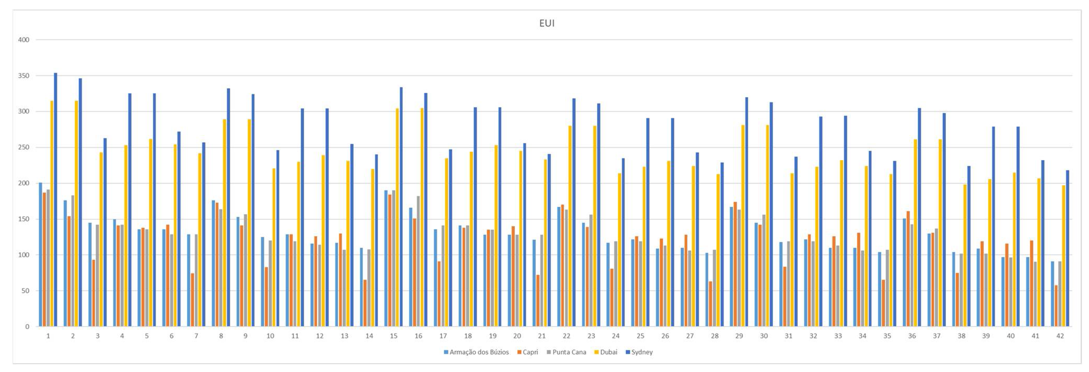
Figure 6 exposes the various results acquired from the simulations, to show the variations on the EUI graphically depending on the different combinations of factors and under the influence of the climate of the different cities analyzed.

The X-axis represents the different sets of combinations (considering that they were 42). It can be seen that in every combination (1, 2, 3, …, 42) exist five bars, which represent the five locations in the assessment process, being light blue for Armação dos Búzios, orange for Capri, grey for Punta Cana, yellow for Dubai and dark blue for Sydney. Y-axis represents the EUI values, which is the measure of the energy consumed in the house of the case-of-study, per square meter, per year.

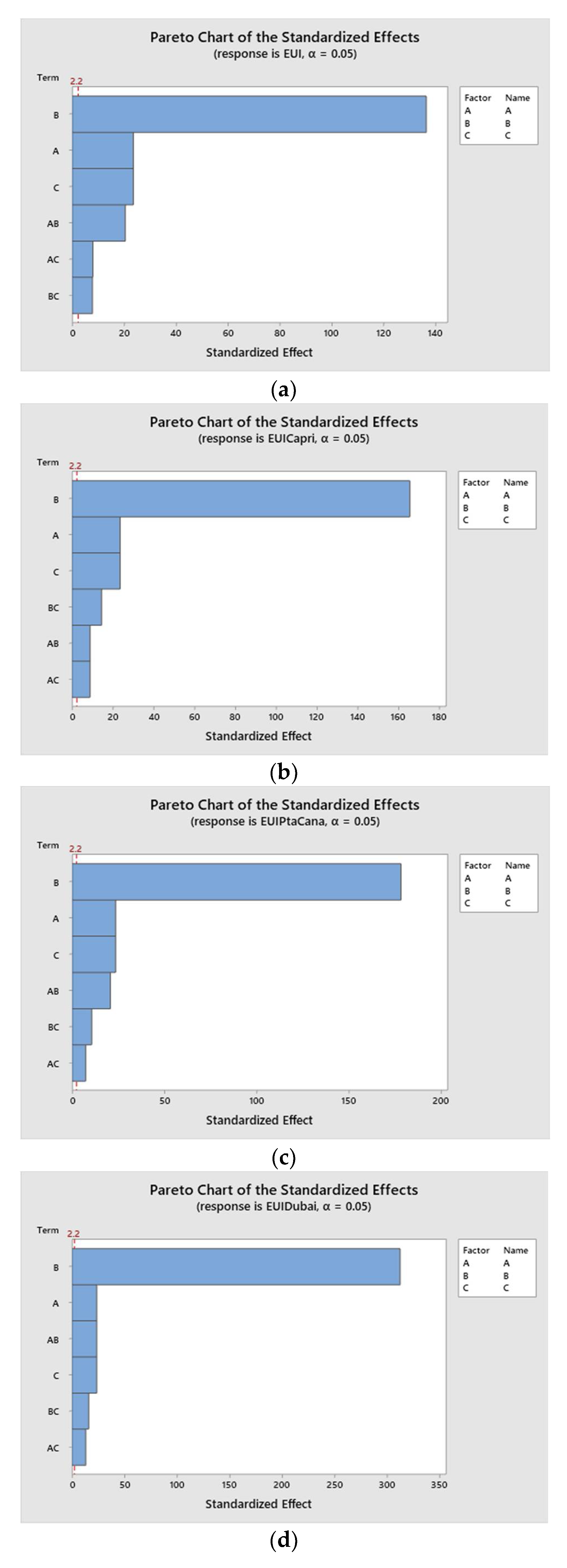
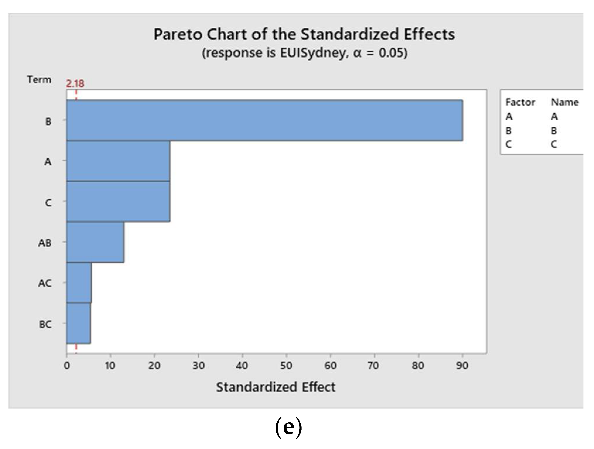
Also, the statistical analysis of the results was executed using Minitab software as the tool to accomplish the study. All of the results are presented in Supplementary Materials; to explain the accuracy of the analysis for each city can be revised the coefficients, variables and formulae from Tables S1–S25. Also, a series of Pareto’s diagrams plots and Residual Plots can be seen from Figures S1–S5. The five figures indicate the correlation’s significance for each of the five cities analyzed. Factors A refers to lighting efficiency; factors B refers to plug load, and factors C refers to the HVAC systems. Factor AB points to the significance of the relationship between lighting and plug load; factor BC, between plug load and HVAC system; and factor AC between lighting efficiency and HVAC system.

Figure 6 shows the results of the energy performance of the building in the case study by varying the different levels and factors, as explained in Table 9. When evaluating these results, it can be seen that the EUI decreases almost in every simulation, until the seventh one, where it goes back up to repeat the cycle, but this time, with slight minor EUI results than the last set of seven. It is possible to denote that the slight diminution is due to the increase of efficiency in both lighting and plug load (going from 11.95 to 3.23 W/m² in the case of lighting, and from 10.76 to 6.46 W/m² in the case of plug load). It is an important matter that expresses the positive effect on energy performance as the lighting and plug load increases their efficiency.

The EUI variations in the seven simulations set are due to the effect of the efficiency from the HVAC systems. Sequences 1, 2, 8, 9, 15, 16, 22, 23, 29, 30, 36, and 37 have higher values of EUI, which means that the Central VAV and the ASHRAE Package System have minor energy efficiency. Sequences 4, 5, 11, 12, 18, 19, 25, 26, 32, 33, 39, and 40 have the medium values of EUI within the set of 7 simulations; it represents that High-Efficiency Package System and the High-Efficiency Package Terminal AC show medium energy efficiency. Sequences 3, 6, 7, 10, 13, 14, 17, 20, 21, 24, 27, 28, 31, 34, 35, 38, 41, and 42 have the lower values of EUI, which illustrates that High-Efficiency Heat Pump, High-Efficiency VAV and ASHRAE Package Terminal Heat Pump are the HVAC systems that display the greatest energy efficiency.

The minor values of EUI are shown in sequence 42, which exhibit the more efficient loads for lighting and power of the equipment, and the ASHRAE Package Terminal Heat Pump (must efficient HVAC system). In analog form, the major values of EUI are shown in sequence 1, which presents the higher values of lighting and power loads (less efficient), and the Central VAV system, which is the most energy-consuming HVAC system. The variation of EUI values between these two sequences is around 100 and 140 kWh/m²/year of difference, which is a significant amount of energy.

Special attention must be given to the fact that the minor values of EUI in every set of seven sequences are found in sequences 7, 14, 21, 28, 35, and 42, confirming that the most efficient HVAC system is the ASHRAE Package Terminal Heat Pump. Same case, the higher values of EUI are expressed in sequences 1, 8, 15, 22, 29, and 36, indicating that the less efficient HVAC system is the Central VAV. It is outstanding that efficiency is needed to improve energy performance, not only for the HVAC system but also for lighting and power devices.

It could be evidenced when comparing sequences 11 and 12 with sequences 18 and 19. Although they have almost the same EUI values, the lighting efficiency increased (from 11.95 to 7.53 W/m²), and the power load efficiency decreased (from 6.46 to 10.76 W/m²). The same thing happens when comparing sequences 25 and 26 and sequences 32 and 33. They present the same HVAC systems (High-Efficiency Package System and High-Efficiency Package Terminal AC) and around the same values of EUI, even when increasing lighting efficiency and decreasing plug load efficiency.

Also, it must be highlighted that efficiency in HVAC systems is representative. The HVAC system considered in sequence 6 (High-Efficiency VAV), which have lower efficiencies in lighting and power loads, produce almost the same effect in the values of EUI shown in sequences 39 and 40, in which the lighting and power load efficiencies diminishes from 11.95 and 10.76 to 3.23 and 6.46 W/m²; it increases to balance the effects of less efficient HVAC systems (such as High-Efficiency Package System and High-Efficiency Package Terminal AC).

The values of energy loads obtained in Figure 6 verify that the combination of efficient lighting, power equipment, and HVAC systems together result in a real diminution of energy consumption and better energy performance. However, climate conditions highlight that could exist a significant variation in the different cities analyzed, even when using the same arrangement of lighting, power load, and HVAC systems’ efficiencies. There is a considerable difference in energy performance for the same sequences due to different locations’ conditions, mainly between the first three climates: Tropical Savanna, Tropical Monsoon and Mediterranean Hot Summer, and the last two climates: Hot Desert and Humid Sub-tropical.

Armação dos Búzios, Punta Cana and Capri presented little variation between them on the EUI results (around 190 kWh/m²/year for sequence 1). Dubai and Sydney showed quite higher energy consumption (around 330 kWh/m²/year also for sequence 1), being possible to denote that EUI for Sydney is the highest in each one of the 42 different sequences (reaching maximum EUI values around 350 kWh/m²/year for sequences 1 and 2). Despite Capri and Sydney present the most variability in sun hours along the year, which can be thought of as more lighting consuming, still showing a wide difference in EUI; for example, in sequences 7 and 12, the gap between Capri and Sydney is 182.7 and 178 kWh/m²/year of EUI respectively. It means that the relevant energy consumption occurs due to the energy required by HVAC systems.

The minor values of EUI for Capri (understood as the city that displays the slight energy consumption results) are found in sequences 7, 14, 21, 28, 35, and 42, which have the most efficient HVAC system (High-Efficiency Package Terminal AC), as aforementioned. However, in some cases, the energy consumption in Armação dos Búzios or Punta Cana could be lesser than in Capri (sequences 5, 6, 12, 13, 19, 20, 22, 25, 26, 27, 29, 32, 33, 34, 36, 39, 40 and 41). Two reasons could explain it.

The first reason is that some HVAC can be more profitable following some climatic conditions (High-Efficiency Package Terminal AC and High-Efficiency VAV can be evidence for being the same two HVAC systems in sequences 5, 6, 12, 13, 19, and 20). The second reason is that when lighting and plug load efficiency increase, the weight of the EUI settles in the HVAC systems (evidenced in sequences 22, 25, 26, 27, 29, 32, 33, 34, 36, 39, 40, and 41); it represents that lighting efficiency and its relationship with sun hours has its significance in energy consumed.

Another indication that some HVAC is more useful in some climatic conditions than others, and lighting efficiency is representative, is that, for Sydney, in sequences 8 and 9, the EUI results are minor (332 and 324 kWh/m²/year) than in sequences 15 and 16 (334 and 326 kWh/m²/year), which present higher lighting and plug load efficiency. In addition, in Dubai, there is no difference in EUI results for sequences 1 and 2, 8 and 9, 22 and 23, 29 and 30, and 36 and 37, even considering the two different HVAC systems (Central VAV and ASHRAE Package System). It is another evidence that some HVAC systems are more profitable in some locations regarding energy consumption.

The behavior analyzed related to the different EUI results for the same sequence evidence that the more variability in the air temperature (around the day and the year), the more energy consumption. It is due to the need for heating and cooling, which became more necessary when presenting wide variations of air temperatures. Furthermore, sun radiation and precipitations regime also show significance in the results. For tropical climates, the EUI does not present significant variations; when having similar climates, the energy consumed will move around the same values due to levels of radiation, clouds presence, and the little variance of air temperature and humidity values.

When interpreting the sequences of every seven simulations in Figure 6, it can be perceived that the energy use intensity seems to decrease when increasing the efficiency of the HVAC system, which is the most representative of the factors. In addition, it can be evident that for tropical climates, the energy consumption is lesser than for desert or sub-tropical climates. However, when the results are introduced in the Minitab software for its linear regression analysis, and making a comparison of the five different Pareto’s diagrams, under the five different cities selected, the results show that HVAC systems are not the only factors that affect the most the EUI results, but also power loads, as seen in Figure 7.

Figure 7a–d expose that the most representative values of effects are for factor B, which is referred to as the Power Loads. It could mean that the power loads increase the EUI equation (which can be demonstrated in Figure 7a–d, which exposes the equations for EUI) in a form even higher than does by the HVAC systems or the lighting loads. Nonetheless, when checking Figure 7e for Sydney, it can be perceived that factor B decreases its effect. It could mean that power loads are not as representative as for the other locations for this specific location. It does not mean that the significance of the other factors (HVAC system or Lighting) is superior for power loads; it could mean that the significance of those factors increases for Sydney.

The statistical analysis accomplished in Minitab can be revised in the Supplementary Materials. In there it is possible to observe the results of the General Factorial Regression, and how its methodology was followed, being possible to obtain the factor information, which describes the division of factors and levels; the analysis of variance, where are showed the information of the p-values; the summary of the model, with the S and R values; the coefficients summary, showing the T-values and p-values and coefficients for each one of the interactions between levels; and finally, the Regression Equation, which expresses the significance of the interactions between factors and levels. By motives related to the size of the regression equation and the coefficients’ tables, this information can be seen more accurately in the Supplementary Materials from Tables S1–S25.

As seen in the Supplementary Materials’ tables, all the p-values of the statistical linear regression analysis are lower than 0.05; it means that the results are truly representative. The normal probability plot of the residuals for Búzios and Capri shows a one-direction tail, which means a normal distribution of the results. For Punta Cana and Sydney, the distribution softly draws an inverted S-curve, which expresses that the distribution of the results is not so normal, due to the variance of the data. For Dubai, the residuals are grouped in vertical lines, which means a greater variation of the values.

When comparing the residuals versus its fits (Supplementary Materials Figures S1–S5), it can be seen that the points are randomly distributed around the 0 for the Dubai and Sydney, more distributed closer to the lower values of EUI in Búzios and Punta Cana, and more distributed closer to the higher values of EUI in Capri. It means that more variance of the results is found for minor EUI results in Búzios and Punta Cana and the major EUI results in Capri.

For Capri and Punta Cana, residuals versus order are randomly distributed around the graphic, which means a typical behavior of the EUI results. For Búzios and Sydney, the graphic shows a tendency to reduce residual values in the middle, having more accurate values in medium EUI results. For Dubai, the graphic displays a tendency of rising residuals in the middle values, which means that the extreme values of EUI present more accuracy. When analyzing these results with the other plots (Supplementary Materials Figures S1–S5), it is possible to comprehend that, even with some variation, the distribution of the residuals is relatively symmetrical, displaying a normal behavior in the results of EUI analyzed.

6. Discussion

This research aids in evaluating the energy performance of a building by manipulating its options of lighting and plug load efficiencies and its types of HVAC systems. Sometimes underestimated, appliances have meaningful importance in energy consumption during the operational phase of a building. A hypothetical house compiling the features presented in single-family, high-income households in Brazil (wide windows, uninsulated walls, clay-roof tiles, open spaces, among others) was analyzed to consider its advantages in the energy consumption of the building when related to the loads of the mentioned facilities.

The model’s design is representative of Brazil, where similar houses are widespread all over the country, same as for other warm-climate zones in America, like the Caribbean. Nevertheless, it may not be similar to households present in Australia or some other sub-tropical zones due to the differences in the construction techniques or material properties. The model analyzed was extrapolated to other locations with the purpose of applying the statistical-experimental design approach as a form to acquire the minimum results of energy consumption.

The results obtained demonstrated the impact that efficiency has on the appliances of a building: the higher the efficiency, the minor the EUI. Comparing the different combinations of design factors and levels between different cities (with different climates), it becomes evident that appliances’ energy consumption could be greater or inferior in some locations. It is caused by the regime of utilization as much as the appliances’ efficiency.

The need for cooling in Sydney (eastern coast of Australia) or Dubai (middle east desert) is more representative than it could be Punta Cana (Caribbean Sea), Armação dos Búzios (southeast coast of Brazil), or in Capri (Mediterranean Sea). Figure 8 and Figure 9 explain this comparison graphically. The different climate conditions with its variables such as air temperature, sun hours and radiation, humidity and precipitation, play an elemental role in defining the energy performance of a building due to the consequent demand for electric demand.

Some values of EUI can be similar between them, as is the case of the EUI for Armação dos Búzios and Punta Cana. It could be explained by sharing the same climate type, but the difference lies in the different sub-climate types and latitudes. The lighting demand must be considered, as presented in Figure 9. Following the duration of sun hours, lighting could be more or less switched on, which impacts energy consumption, mainly in locations with high latitudes, such as Sydney. That is why it becomes necessary they use efficient lights. Also, warm climates demand ventilation devices; for rainy seasons, even without elevated temperatures, humidity has an effect of suffocation.

The building materials and the architectural styles also contribute to improve or worse the energy performance of a building. As evidence, sumptuous, spacious houses adapted to warm climates, as the ones located in Tropical or Mediterranean areas (such as in Armação dos Búzios, Capri, or Punta Cana) has an optimal energy performance (as mentioned by [43,44]), in comparison with the ones located in the desert or sub-tropical climates (Dubai or Sydney). Additionally, the construction materials utilized in the buildings have an important effect on the indoor temperature and consequently in the utilization of HVAC systems to upgrade the comfort, as could be proven in the higher energy demands in Sydney and Dubai, where were utilized the same construction materials than in the mild climate examples.

The link between BIM and BEM methodologies can be accomplished by using Autodesk Revit and its complements Autodesk Insight and Green Building Studio. It can be done simply when clicking on the buttons that perform the analyses. All the difficulties appointed by Gerrish, Miller, and Azevedo [4,16,17], and others can be avoided when working inside the Autodesk Environment. The results emitted by Autodesk Insight are trustworthy, and its versatility of use makes it an advantageous solution for creating energy models starting from a 3D physical model.

An optimal arrangement of lighting, plug loads, and HVAC systems, which could present a differential energy efficiency, diminish in a significant way the energy demand of a building. Considerations about the climate type in the location need to be done for better energy performance. In behalf of this, Experimental Design appears as an optimal choice for a statistical approach of the results when comparing, as in this case, the EUI of the different cases in virtue of a better decision-making process [49]. The analysis made in Minitab software permitted identifying the hidden behavior of the factors that influence the EUI results. The significance of these factors that compose the equation is relevant to know the possibilities of improving or considering changes in the decision-making process.

In addition to this approach, other measures need to be followed to increase sustainable conscience and responsibility. Consume habits also play an important role in energy consumption. The more electric equipment plugged in, the higher the energy demand. Environmental education for changing consumption habits is fundamental, and the substitution of conventional to energy-efficient devices are alternatives that need to be popularized. Insulation strategies, passive architecture measures are also alternatives for improving comfort and reduce energy consumption.

7. Conclusions

Assessment of energy performance appears as an option to improve the energy consumption towards NZEB parameters of sustainability. The appliances within a building have a considerable impact on the energy demand of a dwelling as a part of the operational phase of its life cycle. When diminishing the energy demand, the savings have a positive impact on the environment. The novelty of this research was to apply the linkage between the BIM and BEM methodologies within one environment: Autodesk and its tools REVIT (for performing the physical model) and Insight and Green Building Studio (for performing the energy model) to decrease the energy load of the appliances by applying the experimental design methodology. The results obtained were satisfactory and showed a broad range of options to improve the energy performance.

The analysis contemplated the lighting and power load efficiencies and the HVAC systems, whose options can be easily modified inside the model in REVIT. For preparing the simulations, some variables emitted by Insight remained unchanged, such as construction materials, window-wall ratios, glass types, photovoltaic options, among others, and only were modified the options for lighting efficiencies, power loads efficiencies, and HVAC systems that offer minor energy consume. Because the goal was to decrease the EUI results, a statistical approach was devised to define the options (later called design factors and levels) that could accomplish this intention. Experimental Design was the procedure utilized to create these arrangements via a series of simulations executed in Autodesk Insight to determine the different results of EUI, and a Linear Regression and Analysis of Variance performed in Minitab to analyze the correlations and significances of the variables studied. When evaluating an energy model, it is important to use a statistical linear regression to better understand the factor’s behavior that modifies the EUI and its relation and effects between themselves.

The results obtained could increase or preserve the high indoor comfort levels that the house performs by the architectural concept and reduce energy consumption. In consequence, the environmental impact generated by high energy consumption is also lessened. Considering this panorama, the goal of having a nearly zero energy house presenting opulent features can be achieved more easily.

The selected case study has its particular features, and, despite it is similar to Brazilian bulky houses, its application as a real physical model in other world locations to obtain similar results needs to be studied and improved, adapting to the requirements needed in the location. However, the applied methodology is valid for usance in any other model, where the diminution of the energy loads needs to be achieved.

Some limitations were presented in the research. The lack of information about the materials’ thermal properties did not permit an accurate specification of some other materials. The climatic conditions established by the meteorological stations included in the database of Autodesk REVIT were defined without verifying their accuracy. The options for energy performance improvement, obtained by Autodesk Insight, were considered as they appear in the results, with a lack of knowledge about its viability or specifications. However, the framework can be easily followed for its replication in another research. The specifications about materials, climate conditions in different locations, lighting, power equipment, and HVAC systems loads can be improved and performed for further studies.