Application of Machine Learning for Predicting Building Energy Use at Different Temporal and Spatial Resolution under Climate Change in USA

Abstract

Given the urgency of climate change, development of fast and reliable methods is essential to understand urban building energy use in the sector that accounts for 40% of total energy use in USA. Although machine learning (ML) methods may offer promise and are less difficult to develop, discrepancy in methods, results, and recommendations have emerged that requires attention. Existing research also shows inconsistencies related to integrating climate change models into energy modeling. To address these challenges, four models: random forest (RF), extreme gradient boosting (XGBoost), single regression tree, and multiple linear regression (MLR), were developed using the Commercial Building Energy Consumption Survey dataset to predict energy use intensity (EUI) under projected heating and cooling degree days by the Intergovernmental Panel on Climate Change (IPCC) across the USA during the 21st century. The RF model provided better performance and reduced the mean absolute error by 4%, 11%, and 12% compared to XGBoost, single regression tree, and MLR, respectively. Moreover, using the RF model for climate change analysis showed that office buildings’ EUI will increase between 8.9% to 63.1% compared to 2012 baseline for different geographic regions between 2030 and 2080. One region is projected to experience an EUI reduction of almost 1.5%. Finally, good data enhance the predicting ability of ML therefore, comprehensive regional building datasets are crucial to assess counteraction of building energy use in the face of climate change at finer spatial scale.

1. Introduction

Urban areas account for nearly 67% of total energy consumption worldwide [1]. As the population shifts from rural areas to cities, the energy consumption in cities will continue to rise [2,3]. Understanding energy use in cities and associated greenhouse gas emissions, is critical to solving energy and policy goals. Yet data related to urban energy use is disparate and diverse, especially in the area of building energy use. In London buildings consumes 61% of the city’s energy which is two times higher than the share of transportation [4]. Further, the rising dependency of city residents and workers on appliances, office equipment, and space conditioning has led to the increase in building energy use [1,5]. For example, space conditioning comprises almost 31% of the total energy use of Shanghai, China [6]. Given the pressing nature of climate change, there is an immediate need to develop fast and reliable methods to understand urban building energy use in the sector that accounts for 40% and 30–40% of total energy use in USA and the world, respectively [7,8,9].

Urban buildings are comprised of many types, from residential to commercial, and the fabric of the urban environment is shifting as new buildings are constructed, while existing buildings remain unchanged or are renovated. Understanding the energy use of existing buildings remains challenging as their vintage, material properties, and renovations lead to a high uncertainty in predicting building energy use.

In addition to these challenges, climate change will exacerbate building energy use modeling and predictions. Climate change and extreme weather events like heat waves may have positive or negative effects on energy use of this sector. Therefore, analyzing buildings at large scale and how they consume energy during operation in accordance to different factors such as weather condition, geographic region, building activity (use type), etc. will improve our understanding and aid policy makers and city planners in making informative decisions regarding regional energy and climate change mitigation policies as well as resiliency planning [10,11,12].

Machine learning (ML) may offer promise, and several researchers have explored this space in the context of building energy use [13,14,15,16,17,18,19,20,21,22]. ML approaches are less difficult to pursue than physics-based approaches that rely on heat and mass transfer and requires extensive “input” information [14]. However, disparate methods, databases, temporal resolutions, results, and recommendations related to ML have emerged. Thus, the body of literature was reviewed to analyze gaps and opportunities.

Ahmad et al. established a comparison between artificial neural network (ANN) and random forest when predicting energy use (energy for heating, cooling, and ventilation) of a hotel with hourly resolution [13]. They used ten predictors that presented weather condition, time, and booking status. Through a stepwise technique, hyperparametric ability of ANN and random forest were explored in order to introduce the models’ controls (number of hidden layers for ANN, depth of trees and number of tested predictors at tree nodes for random forest) that provided the closest predictions [13]. Yalcintas et al. used ANN and multiple linear regression (MLR) models to predict office buildings’ electricity use in nine USA census divisions, separately [23,24]. The input predictors that were used in their ANN models varied from those that were used in the MLR models to achieve the best possible predicting performance. Among the predictors only age and number of floors were related to buildings and remaining predictors presented weather condition and operation of buildings [23]. Robinson et al. [25] used Commercial Building Energy Consumption Survey (CBECS) data for training, testing, and evaluating ML models [7]. Then, compared the predictive performance of eleven ML-based models and two linear models that were built using five variables from CBECS. This study reported that extreme gradient boosting provided the best goodness-of-fit in estimating annual energy use. Further, the authors validated this model through applying it to the New York City benchmark dataset and reported that the model performed well on an unseen dataset by having low magnitude of errors [25]. In these studies, ML-based models were reported to provide better performance (lower error) compared to linear models; however, these studies were limited by the numbers and type of predictors used. The diversity of a building’s use type, often used to develop prediction models, is another factor that may affect performance.

Deng et al. selected a subset of CBECS data that was limited to office buildings, and they compared the performance of six models in predicting annual total energy use intensity (EUI), HVAC EUI, lighting EUI, and plug load EUI [26]. Random forest and support vector machine (SVM) were found to have better performance on total EUI prediction; however, different results were reported for other end uses. Errors obtained from different models for HVAC EUI showed great discrepancy; however, for lighting EUI models showed close performance. Finally, the study showed that random forest model had the lowest values of errors for plug load EUI [26].

In order to examine whether addressing the identified gaps have positive effect on prediction accuracy in this study, first, we expanded the scope to all commercial building use types available in CBECS, as Deng et al. focused only on office buildings. Second, our study used more than a hundred predictors via CBECS data to develop our ML models.

In addition to ML disparities and gaps, the existing research also shows inconstancies related to integrating climate change models into energy modeling. Several research projects developed methods and tools to project future weather and studied trends of energy consumption in relation with weather variability [27,28,29,30,31,32,33,34,35,36,37,38], but it is not clear which approach is the most promising as many scenarios present large ranges, making it difficult for decision makers to enact policies. For example, in the thorough work by Reyna and Chester, they employed a physics-based approach to develop a bottom-up model and map the combined effect of climate change and energy efficiency policies for the residential building stock of Los Angeles County (LAC), CA between the years 2020 and 2060 [28]. The stock was clustered into eighty-four archetypes, based on construction period, use type, and climate zone, further electricity and natural gas consumption were simulated utilizing Energy Plus [39]. The morphing technique was used to create hourly weather profiles, for forty-one years, based on four climate change scenarios established by Intergovernmental Panel on Climate Change (IPCC) fifth assessment report (RCP2.6, RCP4.5, RCP6, RCP8.5) [40]. The authors ran numerous simulations and reported results that showed under RCP2.6 and RCP8.5 electricity demand will increase between 41% to 78% and 47% to 87% over different policy scenarios for LAC, respectively.

Similarly, Dirks et al. reported annual buildings energy use of three years (2004, 2052, 2089) based on the IPCC fourth assessment report’s moderate scenario across USA [29,41]. For this study, 26,000 energy models that encompassed a variety of building use types, envelope characteristics, size, etc. and resembled USA building stock were created using Building ENergy Demand (BEND), an energy simulation platform. Dirks and colleagues obtained the downscaled daily precipitation, minimum and maximum temperature, which are required as inputs for energy models, from Computational Assessment of Scenarios of Change for Delta Ecosystem (CASCaDE) dataset. Results for the late 21st century suggested that change in annual electricity use will consistently increase over different census divisions, ranging from 9% to 30%. On the other hand, for mid-century, annual electricity will change inconsistently across different regions ranging from 4% decrease to 19% increase [29].

In another approach, Christenson et al. adopted a method which integrated degree days, building thermal loss, internal gain, and solar gain to develop an equation and quantify the energy demand under climate change in Switzerland [32]. The heating demand was projected to reduce (13% to 87%) for various temporal and spatial spans; however, it was suggested that cooling demand projection needed additional study [32]. In summary, energy use has predicted to rise or lower, with high variations, in different regions over different temporal periods and it deserves further exploration.

The review of existing literature has revealed that there are inconsistencies in the use of ML in urban building energy models. We believe some of the questions remain. At the same time, we acknowledge that drawing general conclusions about algorithms accuracy is not realistic since every data has a unique characteristic. To address these challenges and summarize, robust machine learning methods were applied to predict commercial buildings annual energy use under projected heating and cooling degree days (HDD and CDD) by IPCC across USA during the 21st century. We used publicly available data via CBECS dataset to develop ML models. Specifically, we applied statistical and ML algorithms to the CBECS micro dataset to explore:

1

Which of the statistical and ML algorithms (multiple linear regression, single regression tree, random forest, and extreme gradient boosting) provide a better predictive ability of building energy use intensity by comparing the goodness-of-fit?

2

How many predictors will affect the performance of the model, and what are the type (e.g., age, number of occupants, etc.) and combination of the predictors?

2. Materials and Methods

This section describes the seven phases that were developed and employed to answer the aforementioned research questions. Phase one, data and data preprocessing, clarifies the sources of data and the steps to prepare the dataset, such as predictor selection and feature engineering. In the second phase, a concise characterization of the four models is provided. The third phase, cross validation, focuses on techniques to address uncertainty and minimize bias in developing prediction models. To experiment with the effects of the number, type, and combination of predictors on the accuracy of energy use prediction, three groups of predictors (every group consists of different number and combination) were built (phase four, forming groups of predictors). Phase five, model performance, presents detail information on the metrics that are utilized to validate and evaluate strength of each model in predicting energy use of commercial buildings. These metrics establish the foundation for further comparing and selecting the best model. The next phase uses USA climate regions and census divisions’ boundaries to generate smaller geographic regions with less weather variability, and the visualization of the higher resolution regions is demonstrated. Finally, the climate change phase explains climate change scenarios, obtaining weather projections based on the scenarios, and integration of weather projections into the best ML model to study the energy use change.

2.1. Data and Data Preprocessing

The U.S. Energy Information Administration (EIA) has published ten issues of CBECS since 1979. CBECS is a national-scale survey with a dataset about energy use and parameters that affect energy use of commercial buildings. The dataset is gathered through questionnaires filled out by buildings’ representative or energy suppliers or both parties. This paper used CBECS microdata from 2012 [7]. The micro dataset includes 6720 commercial buildings across USA with detailed information on 491 variables, such as, envelope attributes, mechanical systems, renovation status, operation, occupancy, weather, and energy end use; thus, the variables are either categorical or continuous.

One goal of our work was to include as many commercial buildings as possible, and not focus on a standard commercial office building. We did, however, remove 847 buildings from the CBECS dataset that are more industrial or processing related, these included manufacturing industrial complexes, central physical plant on complexes, plants that produce district steam, plants that produce district hot water, plant that produce district chilled water, plant that produce electricity, and central plants. We conducted interquartile range analysis and removed outliers since regular models are prone to put high weight on outliers that will result in poor performance and low reliability [42]. Based on our experience in building energy modelling, use type plays an important role in the magnitude of energy use; for example, food service usually consumes more energy than office buildings. Hence, an interquartile range analysis was performed for every use type, separately and upper and lower thresholds were estimated based on 1st and 3rd quartiles for all use types [43]. 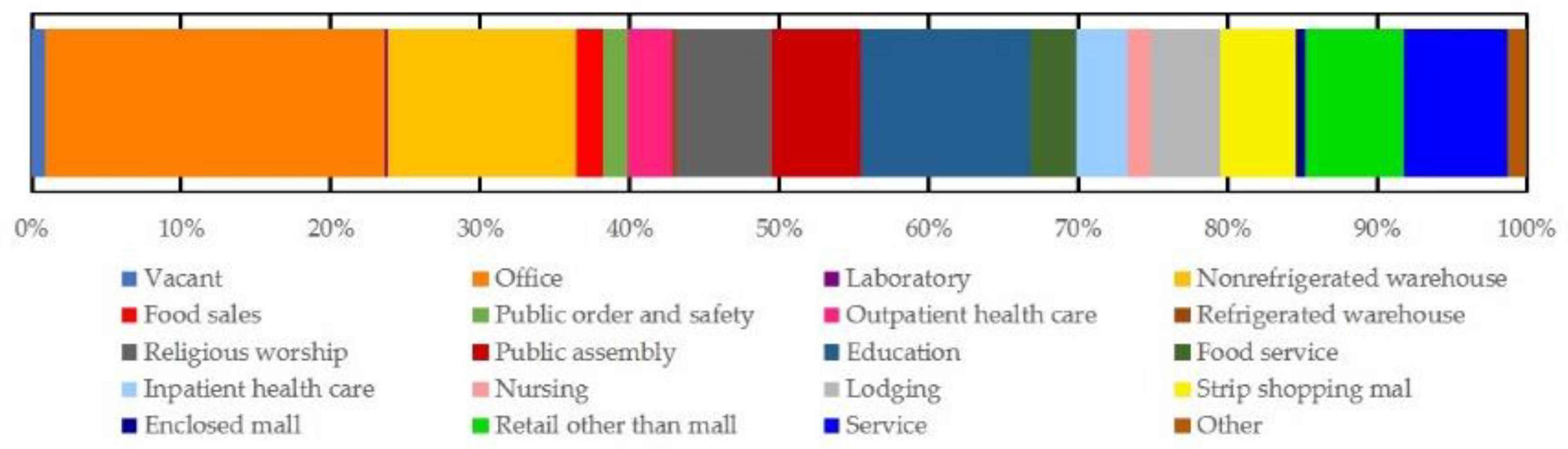Figure 1 shows the frequency distribution of commercial building use types. Ultimately, the dataset included 5252 buildings.

In the development of our models, the input variables are called predictors and the building’s annual EUI is the target variable. The primary statistics of the EUI are displayed in

Table 1. Primary statistics of annual EUI (kBtu/ft²) in the dataset.

Minimum	Maximum	Median	Mean	Standard Deviation
0.0	754.4	57.3	75.9	73.9

.

We developed a list of 114 predictors based on consulting with building energy experts and using building energy modeling [25,26,44].

Table 2. Partial list of input predictors used for developing prediction models. Note: * indicates that the feature engineering technique was applied to the predictors (Table S1 for entire list.). Commercial Building Energy Consumption Survey = CBECS.

CBECS ID	Description	Categorical/ Continuous	Group 1	Group 2	Group 3
HDD65*	Heating degree days	Continuous	✓	✓	✓
CDD65*	Cooling degree days	Continuous	✓	✓	✓
WKHRS*	Total hours open per week	Continuous	✓	✓	✓
NWKER*	Number of employees	Continuous	✓	✓	✓
OE*	Office equipment	Continuous	✓	✓	✓
PUBCLIM	Building America climate region	Categorical	✓	✓	✓
PBA	Principal building activity	Categorical	✓	✓	✓
WLCNS	Wall construction material	Categorical	✓	✓	✓
RFCNS	Roof construction material	Categorical	✓	✓	✓
GLSSPC	Percent exterior glass	Categorical	✓	✓	✓
YRCONC	Year of construction category	Categorical	✓	✓	✓
HEATP	Percent heated	Categorical	✓	✓	✓
COOLP	Percent cooled	Categorical	✓	✓	✓
ENRGYPLN	Energy management plan	Categorical	✓	✓	✓
WINTYP	Window glass type	Categorical	✓	✓	✓

is a partial list of the predictors for brevity, with the entire list of predictors along with descriptions in Table S1. In summary, the dataset includes 5252 observations (buildings) and 114 predictors.

Pre-processing of the data required two steps of feature engineering for continuous predictors and factorial design for categorical predictors.

Feature engineering through scaling was applied to the predictors in Table 2 indicated with an “*” to improve models’ accuracy. Feature engineering converts variables into new forms to be more compatible with machine learning algorithms [45,46]. Equation (1) was utilized for scaling in which $z_i$ is the scaled value of a predictor, $x_i$ is original value of a predictor, $\overline{x}$ is mean of original values, and $\sigma$ represents standard deviation of original values.

$$z_i=\frac{x_i-\overline{x}}{\sigma }$$

(1)

Several categorical predictors have two or more categories, therefore requiring recoding via available techniques (e.g., dummy coding, effects coding, etc.) to be readable by regression-based algorithms [45]. We used dummy coding, which is described as a factorial design that creates pairwise comparisons for categorical variable [47]. A categorical variable with h categories is converted to h − 1 dummy variables. For instance, the principal building activity or use type (e.g., office) is a predictor with twenty categories (1 to 20) which was recoded into nineteen dummy predictors. Every dummy predictor has a value of 0 or 1. Table S3 provides description of categories for all categorical predictors.

2.2. Statistical/ML Models

EUI was calculated via the annual energy use (kBtu) and the floor space (ft²) and is the target variable in our models. The annual energy use is the sum of electricity, natural gas, fuel oil, and district heat as indicated in CBECS.

In order to employ a prediction model for climate change analysis, a determination of what statistical and/or ML algorithm was explored. While there is a broad list of ML models, random forest and extreme gradient boosting were selected to predict annual EUI of buildings. Random forest manages multi-dimensional datasets, that encompass numerous predictors easily and it provides higher training speed compared to other ensemble algorithms, since it can work with a subset of predictors at every node of every tree. Other advantages of random forest are low bias and impartiality regarding non-linear predictors. Likewise, extreme gradient boosting manages non-linearity of data; however, it requires longer training time because trees are formed sequentially (a detailed description of random forest and extreme gradient boosting are provided in subsequent sections). In addition to these advantages, research on predicting building energy use has mostly suggested that ensemble methods provide better performance compared to other ML models or deep learning models such as neural network [13,25,26]. Multiple linear regression and single regression tree were included because they require fewer control parameters; if they provide promising prediction of a dataset, using complex ML models may not be reasonable. Thus, utilizing these four models establishes a sufficient comparison ground. The next sections further describe the four models.

2.2.1. Multiple Linear Regression

Unlike simple linear regression that models a target variable based on one predictor, multiple linear regression finds linear connection between several predictors and a target variable [48]. In general, this connection can be described through the following formula in which k predictors are noted as $x_{i1}$, $x_{i2}$, …, $x_{ik}$, $Y$ is target variable, and ${\alpha }_0$, ${\alpha }_1$, …, ${\alpha }_k$ are regression coefficients, Equation (2).

$${Y=\alpha }_0{+\alpha }_1{x}_{i1}{+\alpha }_2{x}_{i2}{+\dots +\alpha }_k{x}_{ik}$$

(2)

The algorithm determines coefficients through minimizing the sum of square of residual for n observations (every observation constitutes of k predictors and a dependent variable $y_i$) that is described in Equation (3) in which $e_i$ is residual:

$${\displaystyle \sum }_{i=1}^n{e}_i^2={\displaystyle \sum }_{i=1}^n{\left(y_i{-\alpha }_0-{\displaystyle \sum }_{j=1}^k{\alpha }_j{x}_{ij}\right)}^2$$

(3)

2.2.2. Single Regression Tree

A prediction tree aims to model the nonlinear relation between sets of predictors and a target variable through classification if the target is categorical or regression if it is continuous. A regression tree starts from a root node by splitting data into two sub-nodes. In the root node, linear regression is implemented using all predictors to determine the one that partitions data in a way that minimizes the impurity of sub-nodes. The splitting procedure continues recursively at each sub-node until the measured impurity reaches the predefined threshold [49]. The threshold in our model is defined as when data stops converging. Eventually, the value of the target variables at final nodes are averaged and reported as the predicted value of that branch.

2.2.3. Random Forest

Sometimes, results obtained from a single regression tree may show high variance and low accuracy. In order to manage this variation, an ensemble method called bagging has been proposed [50]. In this method, rather than creating one tree based on the original dataset, many smaller datasets consisting of fewer numbers of observations are randomly selected from the original dataset. Further, regression trees are built for every smaller dataset, separately. Ultimately, the predictions from several regression trees are averaged and reported as the final outcome [50].

Random forest, an ensemble ML method, follows the similar strategy as bagging through construction of several classifications or regression trees [51]. The main difference of bagging and random forest is that when splitting nodes of trees, this step is not determined through testing all predictors. If the original dataset includes m number of predictors, m/3 predictors are randomly selected and tested to partition data at each node. For forests which solve classification problems, the number of predictors tested at each node is √m [52].

Since, our model aims to predict annual EUI, a continuous variable, the m/3 predictors are tested at every node of every tree to split data and minimize impurity of sub-nodes. Potential advantages of random forest are reduction in bias and overfitting. However, the required computational power may increase in comparison with statistical models [53].

2.2.4. Extreme Gradient Boosting

Another ensemble method is gradient boosting in which series of trees are constructed. Unlike random forest, trees are not independent. Each tree is formed by learning from the error of the previous tree and tries to improve its performance. The improvement occurs by first forming the loss function of the first tree, which is defined as deviation of the actual and predicted value, Equations (4) and (5), then minimizing the loss function through estimating the negative gradient, Equation (6). The second tree is fitted to the negative gradient and predicted values, obtained from the first tree, and is updated by adding predicted results obtained from second tree. This recursive process continues until the model stops converging or the model reaches predefined number of trees [54]. $y$ is true value of target variable, $F\left(x\right)$ is projected value of target variable, and n is the number of observations in Equations (4)–(6).

$$L=\left(y,F\left(x\right)\right)=\frac{{\left(y-F\left(x\right)\right)}^2}{2}$$

(4)

$$J={\displaystyle \sum }_{i=1}^{n}L\left(y_i,F\left(x_i\right)\right)$$

(5)

$$y_i-F\left(x_i\right)=-\frac{\partial J}{\partial F\left(x_i\right)}$$

(6)

2.3. Cross Validation

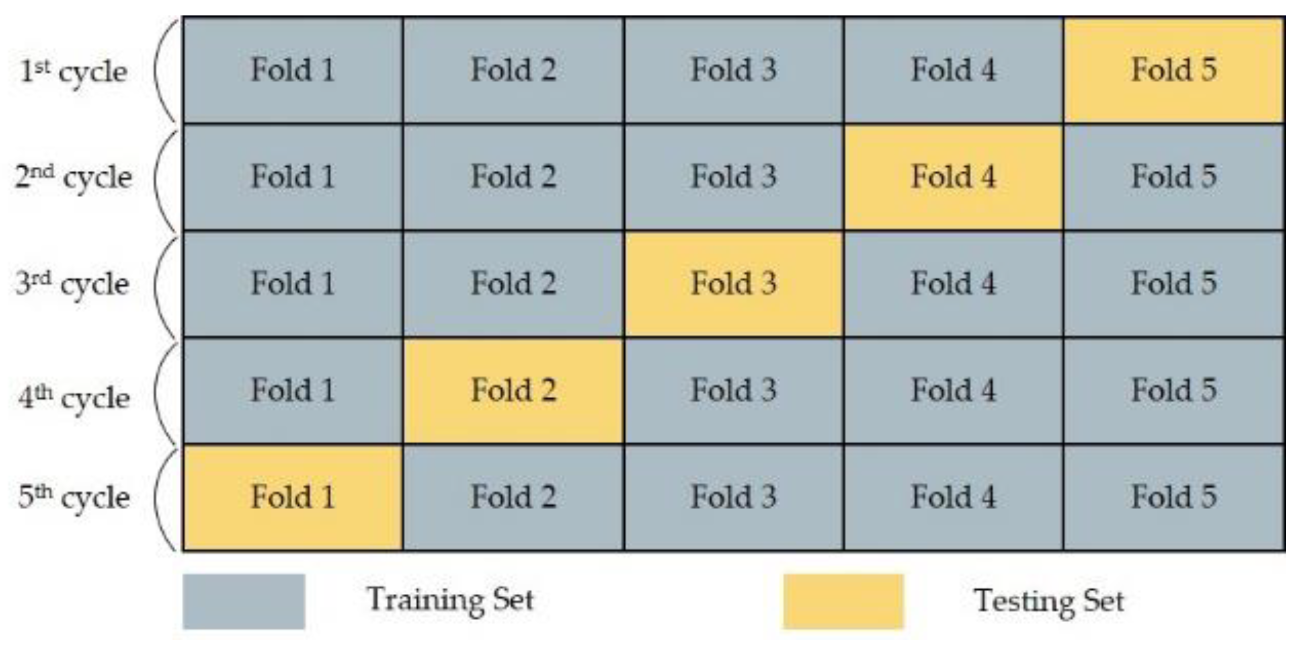
Generally, to reduce bias and address data uncertainty of statistical or ML models, cross validation is conducted. In a k-fold cross validation, the dataset is equally clustered to k folds. For each unique cycle, one-fold is reserved as a testing set and k − 1 folds are combined and serve as the training set. Selection of k should satisfy the tradeoff between the number of sufficient data samples in the training set and testing set.

In this work, we conducted a 5-fold cross validation with over ten rounds of iteration to have sufficient data samples (observations) for testing the models (see Figure 2). The original dataset (group 3, see Figure 3) was divided into five partitions each containing 20% of data samples. Four partitions were considered as the training set for developing a model and the remained one was employed as the testing set to evaluate the efficiency of model on an unseen dataset. Figure 2 shows a summary of cross validation process. For each algorithm, there was a total of fifty models (5 CV × 10 iterations).

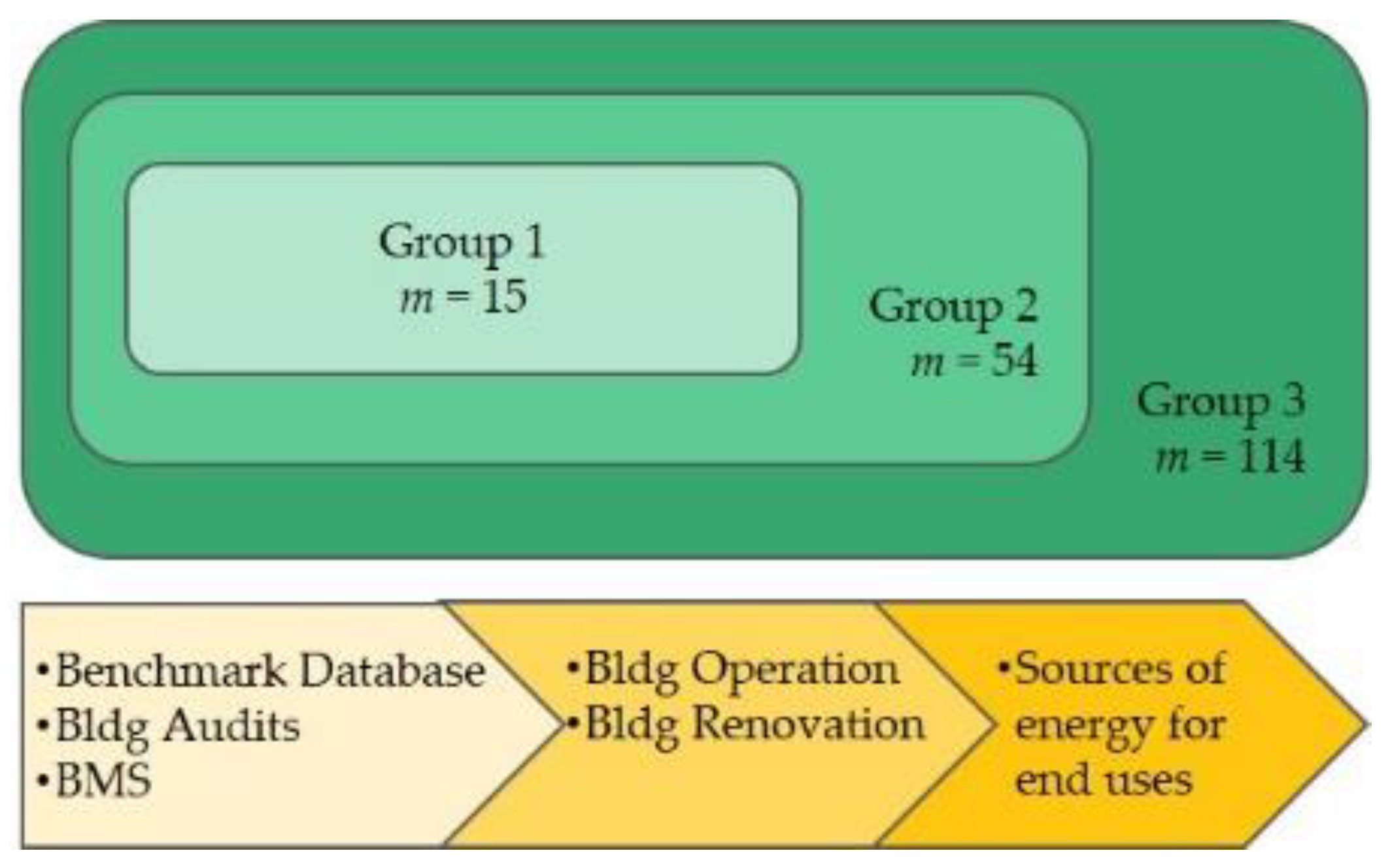
2.4. Forming Groups of Predictors

Previous articles have suggested discrepancies in the number, type, and combination of input predictors may impact the magnitude of prediction errors [25,26]. To explore this issue, we used a stepwise approach in which three subsets of CBECS data were created and used to develop prediction models based on random forest. The first subset which is referred to as group 1 are predictors that are either commonly found in benchmarking databases (e.g., age, use type, HDD, CDD, etc.) or can be obtained by simple building audits and building management systems (e.g., energy management plan, window type, etc.) (see Table 2). Group 2 expands upon the number of predictors in group 1 and encompasses parameters that provide more detailed information about a building’s operation as well as any renovations (e.g., existence of cafeteria, existence of laboratory equipment, lighting upgrade, insulation upgrade, etc.). Lastly, group 3, which is considered as the original dataset, includes all predictors from groups 1 and 2 as well as new predictors that explain sources of energy use for heating, cooling, cooking, water heating, and electricity generation (e.g., district heat used for water heating, electricity used for cooking). Figure 3 displays the relationship of groups 1–3 and a full description of each group is provided in Table S1. Performance metrics of models created for every group are compared and presented in the result of this paper (Section 3.2).

2.5. Model Performance

The common method of evaluating the performance of prediction models in building energy modelling is estimating the errors that are known as performance metrics [18,23,25,26,55,56]. The errors show how the reported EUI varies from predicted EUI obtained from different models. Mean absolute error (MAE), root mean squared error (RMSE), and coefficient of determination (R²) are three metrics that are utilized to select the model that provides the closest predictions to reported EUIs, Equations (7)–(9).

$$MAE=\frac{1}{n}{{\displaystyle \sum }}_{i=1}^n\left|\widehat{y_i}-y_i\right|$$

(7)

$$RMSE=\sqrt{\frac{{{\displaystyle \sum }}_{i=1}^n{\left(\widehat{y_i}-y_i\right)}^2}{n}}$$

(8)

$$R^2=1-\frac{{{\displaystyle \sum }}_{i=1}^n{\left(\widehat{y_i}-y_i\right)}^2}{{{\displaystyle \sum }}_{i=1}^n{\left(y_i-\left(\frac{{{\displaystyle \sum }}_{i=1}^n{y}_i}{n}\right)\right)}^2}$$

(9)

In above equations, $\widehat{y_i}$ is the predicted EUI, $y_i$ is the reported EUI derived from CBECS dataset, and $n$ is the total number of data samples. Every performance metric represents different aspects of variation between reported and predicted values. For instance, MAE explains the average error over entire sample while RMSE penalizes larger errors. Coefficient of determination illustrates the proximity of values to a regression line. Thus, estimating the three metrics establishes a comprehensive foundation for models’ comparison.

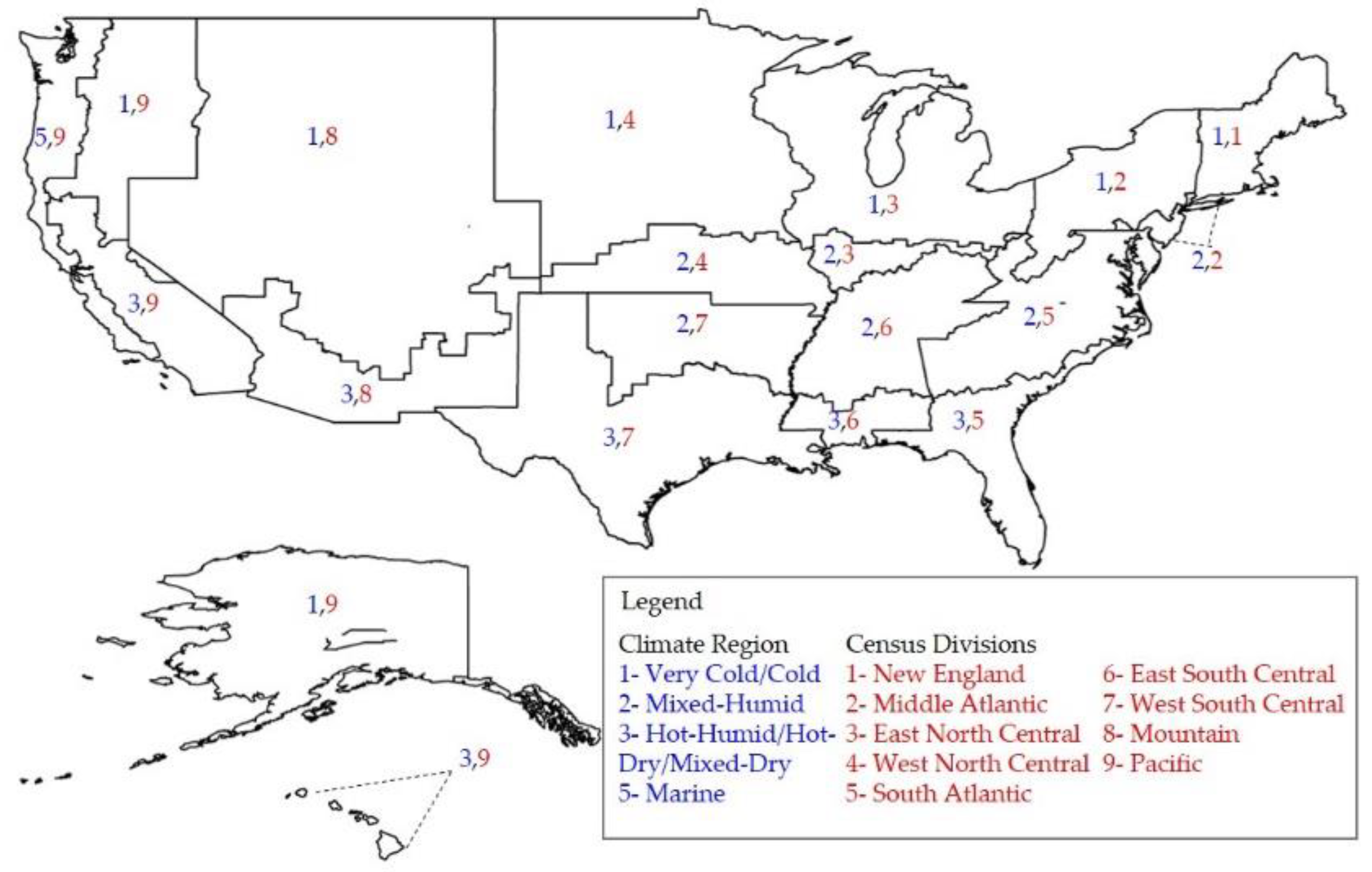
2.6. Integrating Geographic Regions Into Dataset

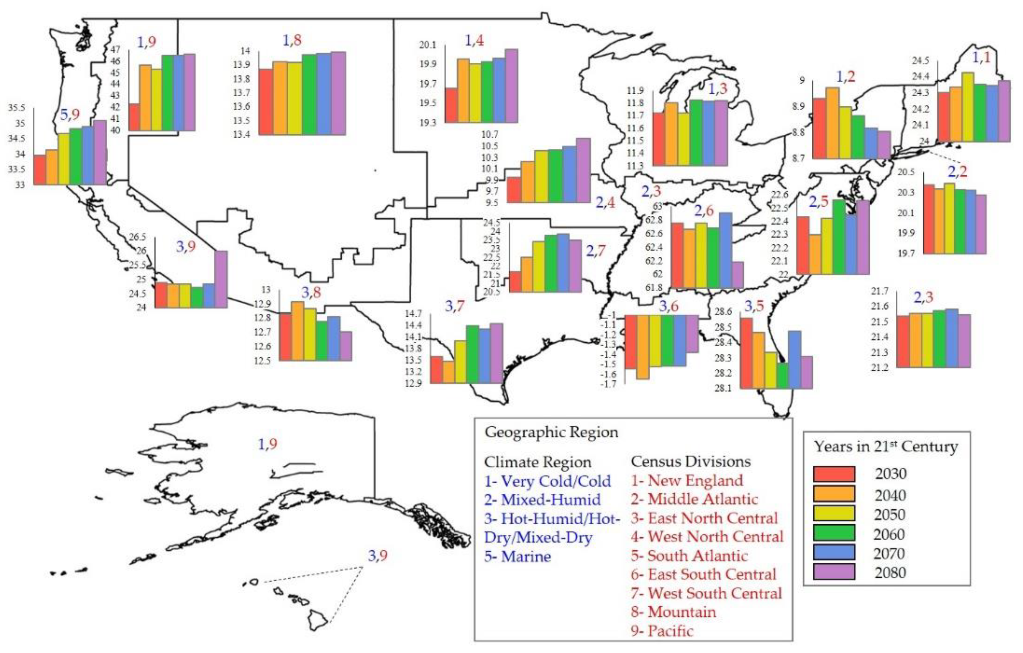
Weather is a key parameter in energy demand of buildings and thus it is always considered in energy and climate analysis. For instance, commercial reference buildings created by U.S. Department of Energy used sixteen climate regions to represent several weather conditions [44]. Unlike U.S. DOE, CBECS used lower spatial resolutions (less specificity with regards to location) to classify climate regions which increase weather variability within the regions. To reduce this variability, defining new boundaries with higher spatial resolution (enhanced specificity with regards to location) is beneficial. In addition, policies regarding climate change are usually established at regional or state level. Thus, in order for the results of our climate change analysis to be interpretable and meaningful for policy makers and planners, they should be aggregated according to these higher resolution boundaries.

The specific location of buildings is not reported in the CBECS dataset to reserve confidentiality; although, two variables in the dataset related to buildings’ location were presented: 1) climate region and 2) census divisions. The 2012 CBECS issue had four categories under climate regions as shown in

Table 3. Coding scheme for geographic regions.

Climate Region (Code)	Census Divisions (Code)	Geographic Region Code
Very Cold/Cold (1)	New England (1)	1,1
	Middle Atlantic (2)	1,2
	East North Central (3)	1,3
	West North Central (4)	1,4
	Mountain (8)	1,8
	Pacific (9)	1,9
Mixed-Humid (2)	Middle Atlantic (2)	2,2
	East North Central (3)	2,3
	West North Central (4)	2,4
	South Atlantic (5)	2,5
	East South Central (6)	2,6
	West South Central (7)	2,7
Hot-Humid/Hot-Dry/Mixed-Dry (3)	South Atlantic (5)	3,5
	East South Central (6)	3,6
	West South Central (7)	3,7
	Mountain (8)	3,8
	Pacific (9)	3,9
Marine (5)	Pacific (9)	5,9

[7,57] and nine categories under census divisions which are originally defined by the Census Bureau. We cross-referenced the two variables to form higher resolution boundaries which are referred as geographic regions in this manuscript.

The cross-referencing process resulted in eighteen geographic regions that are depicted in Figure 4 and the coding scheme is presented in Table 3. Further, every building in the dataset was assigned to a geographic region based on the coding scheme. As an example, a building in a very cold/cold climate that is located in New England has a geographic region code of 1,1. Since the boundary of the geographic regions may not be visually clear in the map (Figure 4), the geographic region codes of all USA counties are provided in Table S2.

2.7. Climate Change

The prediction of the annual EUI of commercial buildings in presence of climate change is one of the primary focus of this study. In this portion of the paper, we first introduce climate change scenarios and then discuss data acquisition.

In the fifth assessment report, IPCC proposed four pathways, known as Representative Concentration Pathways (RCP), RCP 8.5, RCP 6.0, RCP 4.5, RCP 2.6, for the possible range of radiative forcing and associated uncertainties [40]. For each pathway, a concentration of greenhouse gases (GHG) and the radiative forces are projected until 2100. In the most optimistic pathway (RCP2.6), due to the projected concentration of GHG, the radiative forcing is projected to increase by almost 0.95 (Btu/h.ft²) before 2100 and then reduce. Whereas, for RCP8.5 the projected radiative forcing is 2.69 (Btu/h.ft²) by 2100 and maintain an increasing trend after 2100. The radiative forcing will hit 1.43 (Btu/h.ft²) and 1.90 (Btu/h.ft²) by 2100 and will have the same amount after 2100 for RCP4.5 and RCP6.0, respectively. Additionally, the numerical models that are called General Circulation Models (GCMs) can simulate reactions of the climate due to increasing amount of GHG emissions [58,59]. To make the GCM results functional for practical purposes such as regionalization, downscaling methods are usually implemented [30]. For example, National Aeronautics and Space Administration (NASA) used downscaling to create a database, called NASA Earth Exchange Global Downscaled Daily Projections (NEX-GDDP), that contains projection of minimum temperature, maximum temperature, and precipitation under RCP4.5 and RCP8.5 with 15.5 mi × 15.5 mi spatial resolution, which is important when predicting building energy use.

Critical to building energy use is not only the aforementioned regional data, but also degree days. HDD is the summation of the deviation between the average daily temperature and 65 °F over a year, when the average temperature is below 65 °F. CDD is the summation of deviation between average daily temperature and 65 °F over a year when the average temperature is above 65 °F. EIA considered 65 °F as the reference temperature for CBECS. Selection of HDD and CDD as weather variables had two reasons. First, relationship between degree days and building energy use has been proven [60,61,62]. For example, Kennedy et al. showed a correlation between annual EUI and HDD of several countries where increase in HDD led to increase in annual EUI [62]. Second, degree days are almost the only weather-related variables that are available in national-level energy surveys (e.g., CBECS) or regional benchmarking databases.

For this paper, we utilized a publicly available visualization tool, developed by the Partnership for Resilience and Preparedness, a public-private organization working to data accessibly and climate resilience. One of the organization’s key features is that they processed NEX-GDDP raw data and created a visualization tool. For this project, their projected degree days was used for the time period of 2030 to 2080 [63]. Future degree days, as inputs for climate change analysis, are associated with uncertainty. One approach to account for input uncertainty is scenario analysis in which values of input parameters vary over every scenario [64]. Hence, the projected values of HDD and CDD under two scenarios, RCP4.5 and RCP8.5, were imported to the model to address this uncertainty.

Since CBECS does not provide exact locations, the goal was to find locations that have the closest HDD and CDD (for 2012) values to those of buildings in the dataset and use these locations for future HDD and CDD projection for climate change analysis. With this goal, first, the HDD and CDD for the year 2012 along with projected values for six years (2030–2080) of 650 locations in USA were gathered from the visualization tool [63].

These locations were clustered based on the geographic regions (see Section 2.6) in an attempt to build a cross-referencing algorithm with CBECS. The algorithm first identifies a location that has the nearest 2012 values (HDD and CDD) for every building in the dataset. Secondly, it assigns projected degree days for six years in future to every building. In order to ensure that gathered data (labeled population 1) properly represents CBECS’s climatic predictors (population 2), variability of the two populations were tested using F-test. The null hypothesis of this test is the equality of the variance of the two population ($h_o: {\sigma }_1^2={\sigma }_2^2$) which is shown in

Table 4. Results of testing variability of two populations for both HDD and CDD.

Geographic Region	HDD F-Value	CDD F-Value	Critical F-Value	Null Hypothesis
1,1	0.767	0.723	1.471	Not Rejected
1,2	0.737	1.033	1.729	Not Rejected
1,3	1.355	1.383	1.410	Not Rejected
1,4	0.972	1.392	1.432	Not Rejected
1,8	1.403	1.312	1.408	Not Rejected
1,9	1.800	0.730	1.808	Not Rejected
2,2	0.317	0.507	2.342	Not Rejected
2,3	0.964	1.367	3.296	Not Rejected
2,4	0.511	0.644	1.803	Not Rejected
2,5	1.367	1.375	1.498	Not Rejected
2,6	1.153	1.129	1.556	Not Rejected
2,7	1.119	1.279	1.554	Not Rejected
3,5	1.501	0.643	1.565	Not Rejected
3,6	1.481	0.671	2.349	Not Rejected
3,7	0.949	0.582	1.599	Not Rejected
3,8	0.862	1.127	1.751	Not Rejected
3,9	1.234	0.344	2.43	Not Rejected
5,9	1.668	1.464	1.737	Not Rejected

and is not rejected for all regions. This result suggests that gathered climatic data of 650 locations properly represents CBECS. Upon completion of cross-referencing, twelve new datasets (2-scenarios × 6-years) were created and imported to the best fitted model separately to predict EUI.

3. Results

3.1. Performance Validation

Results in

Table 5. Mean absolute error (mean ± standard deviation) of annual EUI for training and testing sets of different models. Performance improvement by comparing random forest model with other models (%) is provided in the last two columns.

Algorithm	Mean Absolute Error (MAE)		Improvement of Random Forest (%)
	Training Set	Testing Set	Training Set	Testing Set
Multiple linear regression	29.80 ± 0.28	31.58 ± 0.89	61.13	12.03
Single regression tree	25.99 ± 0.35	31.25 ± 0.98	55.42	11.10
Random forest	11.58 ± 0.09	27.78 ± 0.75	---	---
XGBoost	27.63 ± 0.50	28.89 ± 0.78	58.07	3.82

and

Table 6. Root mean square error (mean ± standard deviation) of annual EUI for training and testing sets of different models. Performance improvement by comparing random forest model with other models (%) is provided in the last two columns.

Algorithm	Root Mean Square Error (RMSE)		Improvement of Random Forest (%)
	Training Set	Testing Set	Training Set	Testing Set
Multiple linear regression	43.29 ± 0.53	46.07 ± 2.26	61.69	15.63
Single regression tree	36.37 ± 0.58	45.41 ± 2.44	54.40	14.40
Random forest	16.58 ± 0.20	38.87 ± 2.12	---	---
XGBoost	38.87 ± 0.82	41.25 ± 2.52	57.34	5.77

show that ML algorithms outperformed statistical algorithms; furthermore, random forest improved the testing set’s MAE by nearly 12%, 11%, and 4% compared to multiple linear regression, single regression tree, and extreme gradient boosting, respectively. Likewise, implementation of random forest has decreased RMSE by almost 16%, 14%, and 6% in comparison with multiple linear regression, single regression tree, and extreme gradient boosting, respectively (see Table 6). Similarly, R² shows that random forest model has yielded closer linear relationship between reported and predicted EUIs in comparison with other models (see

Table 7. R² (mean ± standard deviation) of annual EUI for training and testing sets of different models.

Algorithm	Coefficient of Determination (R2)
	Training Set	Testing Set
Multiple linear regression	0.66 ± 0.006	0.61 ± 0.029
Single regression tree	0.76 ± 0.006	0.62 ± 0.034
Random forest	0.95 ± 0.001	0.72 ± 0.028
XGBoost	0.72 ± 0.012	0.69 ± 0.034

).

In addition to performance metrics, required computational power may be a crucial factor in selecting the best model. Although the CBECS micro dataset is not considered a very large dataset, it is important to estimate the computational power in terms of total run time for every model, especially because it will be beneficial for future researchers that may work with larger and multi-dimensional datasets.

Table 8. Computational power recorded for different models over ten iterations and 5-fold cross validation.

Algorithm	Running Time (h)
Multiple linear regression	0.28
Single regression tree	0.06
Random forest	5.97
XGBoost	6.13

lists total run time of models using the same central processing unit while no other software programs or applications were in use. Random forest and extreme gradient boosting have more computational power. It is worthwhile to address that the required computational power for hyperparametric models such as random forest and extreme gradient boosting is highly sensitive to parameters that control them for example number of trees, number of predictors tried at every node of a tree, depth of trees, loss function etc.

3.2. Experimenting Impacts of Combination of Predictors on Model Performance

As explained in Section 2.4, three groups were formed to investigate the sensitivity of the model’s performance to the number, type, and combination of predictors. Since random forest (RF) was found as the most promising model in our study (Section 3.1), we aimed to proceed with the sensitivity analysis using RF. Changing the combination of predictors imported into the RF model improved the learning process of random forest. In comparing groups 1 and 2 (Figure 3), the MAE decreased 7% for the training set and 2% for the testing sets. The combination of predictors in group 3 improved the MAE by 15% and 10% for training and testing sets in contrast with group 1 (see

Table 9. Mean absolute error (mean ± standard deviation) of annual EUI for training and testing sets of three groups of predictors (Figure 3) used in the Random Forest model.

Algorithm – Group	Mean Absolute Error (MAE)
	Training Set	Testing Set
Random forest – Group 1	13.61 ± 0.13	30.76 ± 0.95
Random forest – Group 2	12.72 ± 0.13	30.20 ± 0.93
Random forest – Group 3	11.58 ± 0.09	27.78 ± 0.75

). The RMSE’s reduction was equal to MAE’s reduction when comparing groups 1 and 2 (

Table 10. Root mean square error (mean ± standard deviation) of annual EUI for training and testing sets of three groups of predictors (Figure 3) used in the Random Forest model.

Algorithm – Group	Root Mean Square Error (RMSE)
	Training Set	Testing Set
Random forest – Group 1	20.05 ± 0.35	44.23 ± 2.67
Random forest – Group 2	18.72 ± 0.31	43.35 ± 2.57
Random forest – Group 3	16.58 ± 0.20	38.87 ± 2.12

). Comparing groups 1 and 3, RMSE was lowered by 17% and 12% for training and testing sets, accordingly. In like manner, the standard deviations of MAE and RMSE obtained through combination of cross validation and multiple iterations have reduced. Improvements of R² in correlation with combination of predictors and changes in computational power are presented in

Table 11. R² (mean ± standard deviation) of annual EUI for training and testing sets of three groups of predictors (Figure 3) used in the Random Forest model.

Algorithm – Group	Coefficient of Determination (R2)
	Training Set	Testing Set
Random forest – Group 1	0.93 ± 0.002	0.64 ± 0.036
Random forest – Group 2	0.94 ± 0.002	0.65 ± 0.031
Random forest – Group 3	0.95 ± 0.001	0.72 ± 0.028

and

Table 12. Computational power recorded for three groups of predictors (Figure 3) used in the Random Forest model.

Algorithm – Group	Running Time (h)
Random forest – Group 1	1.59
Random forest – Group 2	3.62
Random forest – Group 3	5.97

.

3.3. Impacts of Climate Change on EUI

Deriving from CBECS data, office buildings include the largest portion of commercial buildings by having 18.3% of total floor space [7]. Although our model was comprehensive and included all use types defined by EIA, this section focuses on results obtained for office buildings for the purpose of brevity. Percentage of change in EUI for office buildings under RCP4.5 and RCP8.5 over six years during the 21st century is shown in Figure 5 and Figure 6, respectively. It should be noted that the percent change is averaged over every geographic region separately and the comparison baseline is the EUI in the year 2012.

In region 1,1, EUI will increase almost 24% in 2030 with slight change throughout the century due to projected change in HDD and CDD. The average EUI of office buildings under RCP4.5 will increase by 9% in region 1,2 during 2030. In the same region, energy use is predicted to increase 8.8% in late 21st century under RCP8.5. Likewise, due to RCP8.5, in region 1,4 there will be 19.6% and 20.1% energy use intensity increase at the beginning and end of the century, respectively. The most drastic EUI change in very cold/cold climate has been predicted for region 1,9 (comprising parts of Washington, Oregon, and California) as result of the highest climate change scenario (42.3% and 46.6% increase at 2030and 2080, respectively).

The largest change across mixed-humid climate is projected for region 2,6 (Tennessee, Kentucky, northern Alabama and northern Mississippi) with average EUI growth of 62.7% during all time spans for both climate change scenarios. As shown in the graphs, EUI fluctuation in this region is not considerable throughout the century (ranging from 62.2% to 62.9%). Although predictions obtained from random forest model show that regions located in the mixed-humid climate will experience almost the same increase or decrease in energy use at late 21st century as early 21st century, the result for region 2,7 shows more variation during the century. In this region based on RCP8.5, office buildings are predicted to consume 1.8% more energy per square footage during 2080 as opposed to 2030 (see Figure 6).

Interestingly, during the 1st temporal period in region 3,6 (parts of south Alabama and Mississippi) the EUI of office buildings will be reduced by 1.5% under RCP4.5 and 1.6% under RCP8.5 (see Figure 5 and Figure 6 for percent reduction throughout the century). Whereas, in the rest of geographic regions within hot-humid/hot-dry/mixed-dry climate EUI is showing an increasing trend. Finally, based on random forest model, EUI will gradually escalate from 34% increase at the beginning of the century to 35.1% increase by the end of century for the marine climate (region 5,9 contains parts of Washington, Oregon, and California) under RCP8.5. These EUI is projected to rise by 34% (year 2030) and 34.7% (year 2080) under RCP4.5 for the same geographic region. The increase projected for 5,9 is consistent with finding by Reyna and Chester [28].

4. Discussion

Since previous studies have drawn a different conclusion from applying ML to various subsets of the CBECS dataset [25,26], we first investigated the performance of simple statistical and complex machine learning algorithms on a subset of CBECS, that contains all commercial building use types and more than a hundred predictors, to single out the one that provides better goodness-of-fit to proceed with climate change analysis. Then, we assessed the ability of the prediction model that was developed using random forest algorithm in capturing the change in energy use intensity of commercial building as result of climate change.

As presented earlier, multiple linear regression model showed higher error rates for training and testing sets compared to ML algorithms which demonstrates the non-linear correlation of predictors and target variable. Although the computational power estimated for multiple linear regression was less than ML models, more convenient development and less power-intensive do not compensate for its poor performance. While the magnitude of MAE and RMSE that were obtained for random forest and extreme gradient boosting were slightly high considering the mean value of annual EUI (presented in Table 1), these results were similar to findings by Deng et al. [26]. For instance, Deng et al. found that MAE and RMSE of random forest were 27.0 ± 1.1 and 35.4 ± 1.8, respectively for a subset of CBECS dataset that only included office buildings. In our analysis, random forest provided marginally better prediction for total EUI than extreme gradient boosting whereas Deng and colleagues showed that both random forest and SVM outperformed other models [26]. We concluded that this difference was probably due to the difference in the combination of input predictors of models which shows that selecting input predictors have impacts on the final outcome and the fact that [26] developed the models for office buildings. Additionally, choice of models’ controls for hyperparametric models such as number of trees, loss function, depth of trees, etc. between two studies is another potential reason for this variation. The better performance of both random forest and extreme gradient boosting was reflective of non-linearity and complex interaction of building-, occupant-, operation-, and weather-related predictors and annual energy consumption of commercial buildings at national scale. We used the random forest model over extreme gradient boosting to proceed with both the experiment (Section 2.4) and the climate change analysis because of the following reasons: 1) lower error rate and higher coefficient of determination as discussed above, 2) less computational power (higher running speed), 3) indifference to non-linear predictors, and 4) more convenient tuning of parameters.

An experiment was conducted in Section 2.4 where three groups of predictors were created. Further, random forest models were developed using every group separately to analyze impact of number and various types of predictors on models’ performance. Results depicted that incorporating building operation- and renovation-related predictors (group 2) in the model improved performance marginally compared to group 1. On the other hand, performance of the model developed for group 3, that contained predictors describing energy sources used for various purposes (end uses) in buildings in addition to other predictors, showed considerable improvement over groups 1 and 2. Thus, it can be concluded that variables that describe energy sources for different purposes for instance “electricity used for main heating”, “natural gas used for water heating”, etc. have high contribution in predicting energy use and enhance the model. We think that this is because energy source may influence the coefficient of performance and age of mechanical, HVAC, and hot water systems/equipment of buildings. Furthermore, these variables aid explaining complicated nature of the dataset. Another finding to be address is that incorporating more input predictors to achieve a better model did not lead to overfitting because training set’s and testing set’s errors (MAE, RMSE,), and R² have reduced and increased, respectively.

As climatic analysis has suggested, EUI of commercial buildings will be affected by changes in two weather-related parameters (HDD and CDD). Most of geographic regions are predicted to have increase in energy use which conveys that increase in cooling demand due to warmer future will exceed the presumable reduction in heating demand. Moreover, space heating requires more energy than cooling [65], so presumable reduction in heating is not significant which will lead to overall energy use increase. Although the impact of changes in HDD and CDD is considerable when comparing energy use intensity of six years throughout 21st century to energy use intensity in the year 2012, changes in energy use intensity between these six years are not significant. We believe that the insignificant changes may be due to two reasons: 1) generalization of ML model, 2) reciprocal effects of building energy use and climate change. A well-generalized ML model is not affected by minor variations of few predictors. In the case of this study, since degree days changes minimally from one year to another year in future, the predicted energy use does not change considerably. However, since degree days is projected to change significantly compared to recorded HDD and CDD for the year 2012, the predicted energy use intensity shows noticeable changes. In conclusion, a well-generalized building prediction model does not reflect minor changes in weather-related predictors on the final target variable. Secondly, climate change in general and variation in degree days in specific are known to be the result of GHG emissions. Since operation of the building sector depends on the combustion of fossil fuels, the main source of GHG emissions, directly (i.e., coal, natural gas, petroleum) and indirectly (electricity generation) [66,67], there is probably a reciprocal cause and effect between variation in degree days and building energy use. This is another reason for insignificant energy use intensity change of six studied years. This possibility opens discussion regarding future work. Outliers, imputed values for some data samples, lack of occupants’ behavior, and complex interaction between predictors and annual EUI in CBECS dataset are challenges of interpretability of the model. In order to solve this challenge and better explain how the prediction model based on random forest has made decisions, SHAP analysis could be conducted in future works. SHAP is a deep learning framework that explains which predictors are more relevant for certain predictions or clarifies overall performance of a model through multiple visual means such as dependence plot, model explainer, and prediction explainer [68,69].

Detail and reliable data enhance predicting ability of ML and artificial intelligent approaches. However, majority of energy benchmarking efforts in USA cities like Philadelphia, New York, etc. lacks information regarding occupant-, operation-, HVAC system-, and weather-related parameters. Therefore, launching movements toward collecting more comprehensive regional building datasets in future is crucial to evaluate counteraction of building energy consumption and climate change at finer spatial scale using ML approaches. Policy makers and urban planners can advocate for allocating budgets to gather building dataset. Also, they can use the results of our study as a future road map of building energy use in presence of climatic variation.