Research on Chip Shear Angle and Built-Up Edge of Slow-Rate Machining EN C45 and EN 16MnCr5 Steels

Abstract

One of the phenomena that accompanies metal cutting is extensive plastic deformation and fracture. The excess material is plastically deformed, fractured, and removed from the workpiece in the form of chips, the formation of which depends on the type of crack and their propagation. Even in case of the so-called ‘continuous’ chip formation there still has to be a fracture, as the cutting process involves the separation of a chip from the workpiece. Controlling the chip separation and its patterning in a suitable form is the most important problem of the current industrial processes, which should be highly automated to achieve maximal production efficiency. The article deals with the chip root evaluation of two EN C45 and EN 16MnCr5 steels, focusing on the shear angle measuring and built-up edge observation as important factors influencing the machining process, because a repeated formation and dislodgement of built-up edge unfavorably affects changes in the rake angle, causing fluctuation in cutting forces, and thus inducing vibration, which is harmful to the cutting tool. Consequently, this leads to surface finish deterioration. The planing was selected as a slow-rate machining operation, within which orthogonal and oblique cutting has been used for the comparative chips’ root study. The planned experiment was implemented at three levels (lower, basic, and upper) for the test preparation and the statistical method, and regression function was used for the data evaluation. The mutual connections among the four considered factors (cutting speed, cutting depth, tool cutting edge inclination, and rake angle) and investigated by the shear angle were plotted in the form of graphical dependencies. Finally, chips obtained from both steels types and within both cutting methods were systematically processed from the microscopic (chip root) and macroscopic (chip pattern) points of view.

1. Introduction

Almost every mechanical component in use has undergone a machining operation at some stage of its manufacturing process. Considering that the economics of the metal cutting process significantly affect the overall cost of the final products, there is a strong drive to reduce the time and cost of machining operations. This is one of the reasons why chip machining technology underwent huge developments in the last several decades, which has been displayed by its massive use in industrial practice. Despite the opinion of some experts [1,2] that the manufacturing of components by machining is not efficient and that it is necessary to substitute it with chip-less methods, this technology is irreplaceable by other technological methods in many cases. The demanded accuracy and the quality of a machined surface are in many cases not achievable by mechanical working or casting processes, because the surfaces of the parts are adversely affected. This is why machining is needed. [3] Controlling the chip separation and its patterning in a suitable form is the most important problem of the current industrial processes, which should be highly automated to achieve maximal production efficiency.

One of the phenomena that accompanies metal cutting is extensive plastic deformation and fracture. The excess material is plastically deformed, fractured, and removed from the workpiece in the form of chips, the formation of which depends on the type of crack and their propagation. Even in the case of so-called ‘continuous’ chip formation there still has to be a fracture, as the cutting process involves the separation of a chip from the workpiece. Chips at the machining are formed due to tearing and shearing, the workpiece material adjacent to the tool face is compressed and a crack runs ahead of the cutting tool and towards the body of the workpiece. Cutting takes place intermittently and there is no movement of the work-piece material over the tool face. In chip formation by shear, there is general movement of the chip over the tool face.

As the tool advances into the work-piece, the metal ahead of the tool is severely stressed. The cutting tool causes internal shearing action in the metal, such that the metal below the cutting edge flows plastically in the form of a chip. Firstly, compression of the metal under the tool edge takes place, followed by the separation of the metal when the compression limit of that metal has been exceeded. Plastic flow takes place in a localized region called the shear plane, which extends from the cutting edge obliquely up to the uncut surface ahead of the tool. When the metal is sheared the crystals are elongated, the direction of elongation being different than that of the shear.

The angle made by a plane of shear with the direction of tool travel is known as the shear angle, Φ. Its value depends on the material being cut and the cutting conditions. If the shear angle is small, the path of the shear will be long, chips will be thick, and the force required to remove the layer of metal of given thickness will be high, and vice versa.

2. State of the Art

The classic shear plane model is based on a free body diagram of the chip, which is held in equilibrium by two equal, opposite, and collinear resultant forces, one acting on a shear plane, and the other on the rake face of the tool. This was developed by Merchant [4] in the early 1940s. Figure 1 depicts the famous Merchant’s circle, which shows the relationship between various force and velocity components acting on the chip. The individual symbols are defined as follows: v_c—chip velocity, v_s—shearing velocity, v_w—workpiece velocity, R_s is the resultant force on the tool with its projections in shear and in frictional directions, α, Φ, and β are the rake, shear, and friction angles, respectively, L_c is the contact length, and h and h_c are uncut chip thickness and chip thickness, respectively.

The basis of the scientific research related to orthogonal machining provided by Merchant has been further developed by many scientists, such as Weiner [5], Wallace and Boothroyd [6], and Muraka et al. [7]. Later, the involvement of computer aid enabled the development of new numerical models of orthogonal machining. The related research has been presented by Li et al. [8], Shi et al. [9], Filice et al. [10], Bagci [11], Priyadarshini et al. [12], and other researchers.

To study chip characteristics, it is necessary to specify the type of machining by which the chip forms. There are two different types of cutting: orthogonal and oblique. Orthogonal cutting is a type of metal cutting in which the cutting edge of the wedge shape cutting tool is perpendicular to the direction of tool motion. In this cutting, the cutting edge is wider than the width of a cut. This cutting is also known as 2D cutting, because the force developed during cutting can be a plot on a plane or can be represented by a 2D coordinate. However, orthogonal cutting is only a particular case of oblique cutting, such that any analysis of orthogonal cutting can be applied to oblique cutting. Oblique cutting is a common type of three-dimensional cutting used in the machining process [13].

The characterization of chip morphology is defined by analyzing the chip, both on a micro and macro level. On a micro-level, the chip is characterized as chip shape and at the macro level as chip curl. The chip shape characterizes the chip’s cross-section in a plane perpendicular to the rake face and the cutting plane. Continuous chips, segmented chips, and discontinuous chips could be defined as the most important classification of chip shape and this is influenced to a large extent by workpiece material behavior, cutting process parameters, and cutting tool macro geometry [14]. Mathematical formulations employing the above defined geometrical parameters were later developed by Nakayama et al. to define the chip in 3D practical applications [15]. A more systematic study on chip curl was developed by various research groups over several decades [14,16,17,18]. In addition, chip curl research has been well-reviewed and documented [19,20] and has resulted in a more quantifiable chip form classification. Among all these fundamental influences, from a cutting tool geometry viewpoint, the cutting tool macro geometry influences chip curl to a large extent. 2D orthogonal cutting would primarily result in an up curled chip, with side curling to a very small extent. In 3D oblique cutting, chips are a combination of both side curl and up curl. Chip curl is also influenced to a large extent by the nose configuration and its effect is dependent on the relationship between the nose radius and process parameters selected [21]. Chip segmentation is of pivotal importance, since it facilitates the machining ergonomics and scrap removal without damaging workpiece surface quality and ensuring the safety of the working personnel [22].

Noteworthy studies within the chip formation field are the works of Shaw et al. [23], Luk [24], and Okushima and Minato [25]. Palmer and Oxley [26] used experimental flow fields obtained by tracing the path of individual grains in low speed cutting to determine the extent of the deformation zone and the shear angle. They showed that the plastic deformation zone has a substantial thickness and the streamlines form smooth curves from the workpiece into the chip. They also developed slip-line field solutions from the experimental results and calculated the stress distribution in the deformation zone. Oxley and Welsh [27] developed a parallel-sided shear zone theory, which allows for strain hardening of the material. In this model, the shear flow stress changes from the initial yield stress at the lower boundary of the shear zone to a higher value at its upper boundary.

Along with an evolution of new materials that should be machined and continual cutting tools improvements, the topic of chip formation and its morphology is still relevant, so many researchers are presently addressing this issue. Prasetyo and Tauviqirrahman [28] developed more comprehensive models by using a power-law flow stress equation, whose coefficients are dependent on strain rate and temperature. These effects were combined using the concept of velocity-modified temperature, and it was suggested that the flow stress for a particular material at a given strain can be assumed to be a unique function of this parameter. Hegab with his research team [29] investigated the effects of two types of nano-cutting fluids on tool performance and chip morphology during the turning of Inconel 718. Similarly, Adekunle et al. [30] dealt with the chip morphology and behavior of tool temperature during the turning of AISI 301steel using different biodegradable oils. Anthony [31] analyzed a cutting force and chip morphology during the hard turning of AISI D2 steel. Their research confirmed the results of other studies, within which it was found that depth of the cut, followed by cutting speed, influence cutting force considerably. Umer et al. studied chip morphology predictions while machining hardened tool steel using finite element and smoothed particles hydrodynamics methods [32]. The topic of chip morphology and its formation modeling during metal cutting operations was also the subject of a study by Mabrouki et al. [33].

In chip machining, the chip forming process is often accompanied by the formation of a built-up edge (BUE) in the face of the tool and it is necessary to take this phenomenon into account. Its creation changes the geometry of the cutting tool and thus the conditions of the cutting process. It affects the removal of the chip from the cutting zone, its twisting, and shaping due to the material sticking to the tool face and thereby causing the tool face angle to change during the cutting process. During chip formation, the material layers of the workpiece become highly plastically deformed, and after separation by friction on the tool face this forms a so-called braked layer between the exiting chip and the tool face. The height of this layer varies considerably, depending on the cutting speed. At very low cutting speeds, the material is not sufficiently heated and plastic to cause such phenomena. However, when machining with cutting tools from high-speed steel at a cutting speed of 10 to 30 m·min⁻¹, these layers can be welded under pressure and thus lead to an increase in the tool face. Figure 2a–d shows the succession of the built-up-edge using the slip lines [34,35].

The tool angles of rake and clearance increase plastically due to the build-up edge (BUE) appearing, significantly increasing the corner radius (from r to r_BUE), depending on the size of the build-up edge. Since the built-up edge plastically extends the cutting edge, it increases the thickness of the cutting layer (from h to h_BUE) (Figure 2e) [36].

The important features of the built-up edge are the variability of its dimensions over time and space (in the line of the cutting edge) and the high hardness that will allow it to assume the function of the cutting edge. There is some range of cutting speed at which the built-up edge occurs. Outside this cutting speed range, no built-up edge can be observed [37,38].

As can be seen from the research works presented above, a great deal of research has been devoted toward understanding the mechanics of metal cutting, with the objective of obtaining more effective cutting tools and more efficient manufacturing process plans. Traditionally, these objectives have been achieved by experimentation and numerical simulation. In spite of extensive research in this field, the basic mechanics of the cutting process and the interplay of many factors which lead to its great variety are not yet totally understood, so the search for more effective models continues on analytical, experimental, and numerical fronts.

This study is an original contribution to the chip root research of two EN C45 and EN 16MnCr5 steel types as one of the possibilities to develop knowledge within a chip fracturing that can minimize cutting-tool wear and poor machinability, restricting the quality and productivity of the machining process. It aims to contribute to the analysis of the chip formation process at orthogonal and oblique cutting with relatively slower speeds, focusing on the chip shear angle and built-up edge investigation, as well as to the finding out the impact of selected machining factors on this process. The planing operation has been selected due to the visibility of the chip formation to the naked eye. This type of machining has also allowed authors to develop a new reliable method for sample acquisition in order to avoid chip root deformation and its thermal influence on sample acquisition, which could cause changes in the microstructure of the material.

To the best of our knowledge, no relevant studies have been published concerning chip root observations and the influence of cutting parameters (cutting speed, cutting depth, tool cutting edge inclination, and rake angle affected by forming built-up edge) on the shear angle of both EN C45 and EN 16MnCr5 steels types within such deep and complex comparative research. In addition, the mutual connections among the four considered factors influencing shear angle in orthogonal and oblique cutting have been plotted in the form of graphical dependencies.

3. Materials and Methods

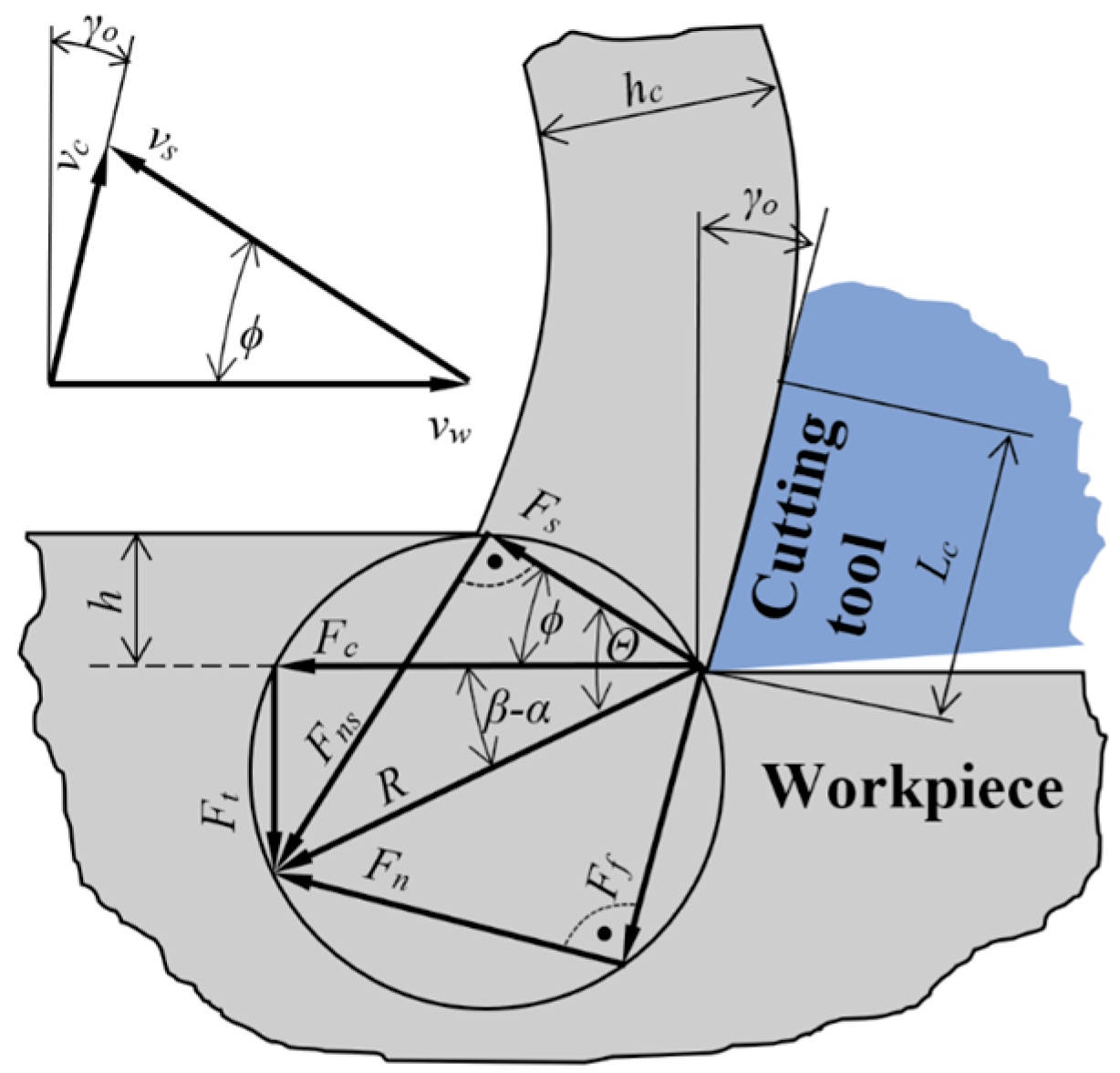
3.1. Cutting Tools, Machined Material, and Measuring Equipment

Chip formation at orthogonal and oblique slow-rate machining has been experimentally investigated within this research. For this study, the technology of planing was selected, at which the main sliding motion performs a workpiece. The machining process was carried out using the planer machine of KOVOSVIT MAS Machine Tools (Sezimovo Ústí, Czech Republic).

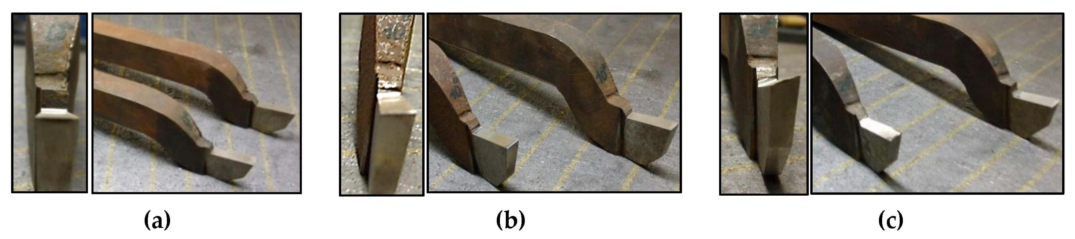
The planing necking tool type 32 × 20 ON 36550 HSS00 (PILANA Tools Ltd., Hulin, Czech Republic) was used for orthogonal cutting and a straight roughing tool 32 × 20 ON 36500 HSS00 was used in oblique machining. Both types of cutting tools included brazed-tips from high-speed steel with three different types of cutting edge inclinations: λ_s = 0°, 10°, and 20°. The angle of tool orthogonal rake γ_o and angle of tool orthogonal clearance α_o were varied in the second and third phase of the experiments to get a better view of the chip formation and to obtain more reliable results. Pictures of the cutting tools are presented in Figure 3 and Figure 4 and their geometries are arranged in

Table 1. Changes in the angle values.

Type of Tool Angle	Planing Necking Tool	Straight Roughing Tool
Tool cutting edge angle κr	0°	60°
Tool minor (end) cutting edge angle κr’	-	20°
Tool included angle εr	-	100°
Angle of tool orthogonal rake γo	8°/12°/16°	3°/7°/11°
Angle of tool orthogonal clearance αo	15°/11°/7°	15°/11°/7°

.

In order to verify the input angles of the tool orthogonal rake γ_o, preliminary input tests were performed. The tests were carried out using 3D measuring equipment RAPID CNC THOME (Zimme Maschinenbau GmbH, Kufstein, Austria), as shown in Figure 5, along with detail from the measuring process.

The angle of tool orthogonal rake γ_o was measured for every cutting tool used in the next experiments. The protocols from the measurements confirmed the values listed in Table 1, while the deviation of all measured values did not exceed 5% and the average angles of tool orthogonal rake for planing necking tools and straight roughing tool were γ_o = 8.138° = 8°2′0″ or γ_o = 3.159 = 3°2′1″, respectively.

The steels 1.7131 (EN 16MnCr5) and 1.0503 (EN C45) were selected as a machined material, the chip formation of which has been subjected to research. The chemical composition of these steels types is presented in

Table 2. Chemical composition of the steels.

Steel	C (%)	Mn (%)	Si (%)	Cr (%)	Ni (%)	Cu (%)	P (%)	S (%)
EN C45	0.42–0.50	0.50–0.80	0.17–0.37	max 0.25	max 0.30	max 0.30	max 0.040	max 0.040
EN 16MnCr5	0.14–0.19	1.10–1.40	0.17–0.37	0.80–1.10	-	-	max 0.035	max 0.035

.

The steel 1.7131 (EN 16MnCr5) contains smooth deformable calcium aluminates, encapsulated in manganese sulphide, as an alternative to tough alumina oxide inclusions. It is suitable for cementing and for die forging; it is well machinable, well weldable, and, after annealing, also well formable. This grade of steel is generally used for elements with a required core tensile strength of 800–1100 N·mm⁻² and good carrying resistance, e.g., piston bolts, camshafts, levers, and other automobile and mechanical engineering add-ons.

The steel 1.0503 (EN C45) is an unalloyed medium carbon engineering steel which offers moderate tensile strengths, wear resistance, and good machinability. This material is capable of through hardening by quenching and tempering on limited sections and can also be flame or induction hardened to a surface hardness of min 55 HRC. C45 is generally supplied in an untreated or normalized condition, with a typical tensile strength range of 570–700 MPa and Brinell hardness range of 170–210.

The infrared thermometer UNI-T UT305C (manufacturer UNI-TREND Technology, China Co., Ltd., Dongguan, China), based on a principle of infrared radiation emitted from the target surface, was used to measure the temperature.

Vickers microhardness was measured with the MICRO—VICKERS HARDNESS TESTER CV—403DAT (MetTech Ltd., Calgary, AB, Canada), which has the possibility of magnifying a view 200 times and 600 times.

Etched specimens of chips were observed by means of the Platinum USB digital microscope UM019 (Shenzhen Handsome Technology Co., Ltd., Shenzhen, China) with magnification 25–220×.

3.2. Methods

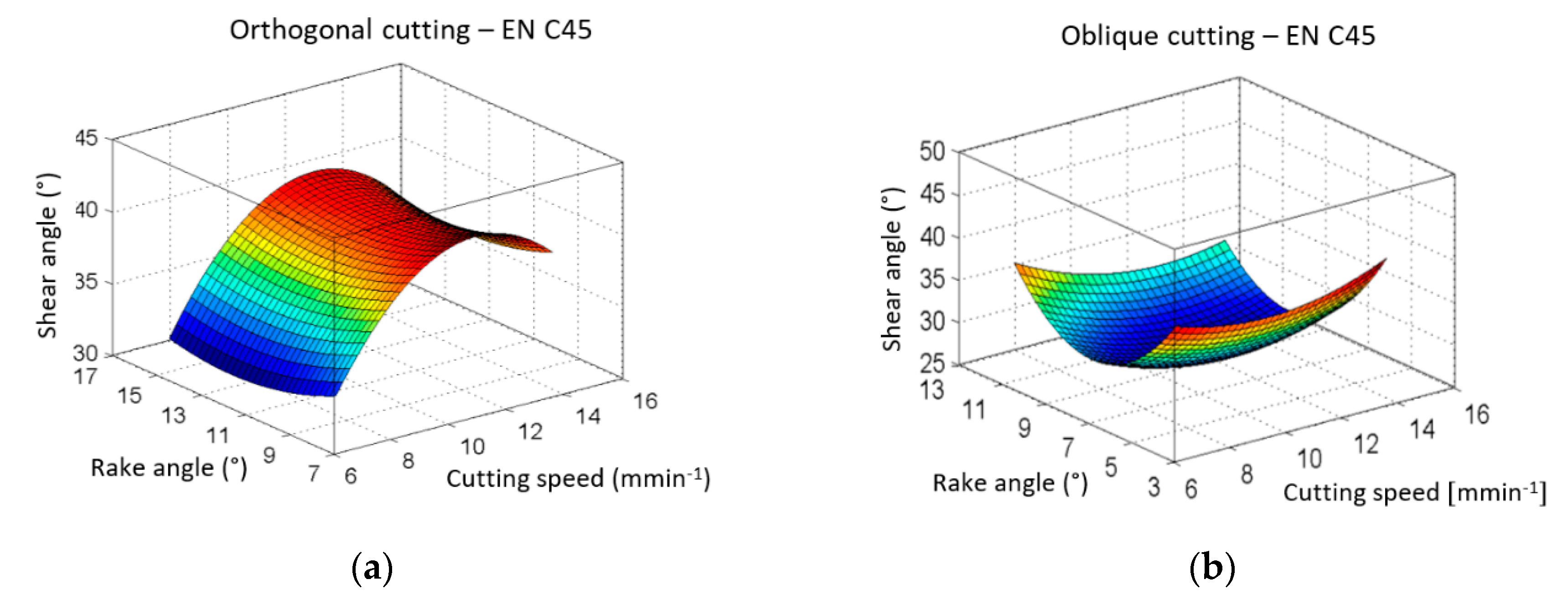
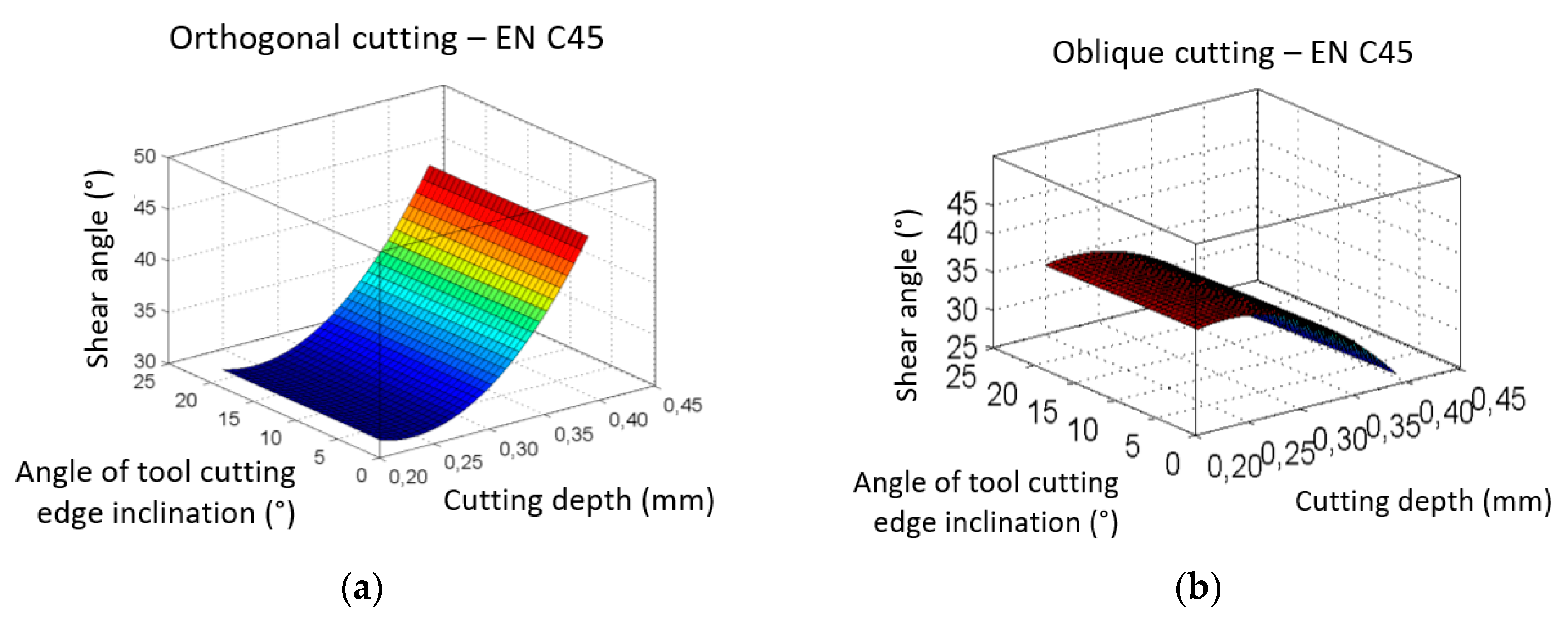
In order to maximize the amount of “information” that was obtained by a given experimental effort, it is necessary to design the experimental plan well. Many experimental designs (full factorial design in two/three levels, fractional factorial design, Plackett–Burman design, Doehlert matrix, A Box–Wilson Central Composite Design, Box Behnken designs, and others) have been recognized as useful techniques to optimize process variables. The influence of four factors (cutting speed, cutting depth, rake angle, and angle of cutting edge inclination) on chip formation (shear angle) in a slow rate machining process was investigated in this study. In this case, the most powerful tool of the planned experiment appeared to be how the basic principle was a measurement of each factor’s influence on three levels [36,39,40].

The description of the experimental plan within this part of the article is given due to a better understanding of measured data processing.

Based on [41], the basic equations for statistical processing can be written in the matrix (1):

Y = X·b,

(1)

where Y—column vector of measured quantities, X—matrix of independent variables, b—coefficient of a regression function.

The system of normal Equation (2) can be expressed in the following way:

[X^T·Y] = [X^T·X]·b.

(2)

The vector “b” in relationship (2) is specified by the least-squares’ method of the matrix regression analysis (3):

b = [X^T·X]⁻¹·X^T·Y.

(3)

It is necessary to consider that the complete three-level plan had a large scale of measurements expressed by N = 3^k, where k is a number of variables (in this case factors) and N is a number of measures (e.g., considering four variables within an experiment, a total of 81 measurements should be performed, because N = 3⁴ = 81) [36].

A reduced number of measurements for the dependencies described by functions of the second order can be achieved by means of the so-called second level compositional non-rotational plan [42], while the symbols in Equation (4) have the following meanings: x_j is a variable (in the case of presented research it is one of the cutting parameters that will be varied), j, u are indexes that define a parameter, b_j is a j-th correlation coefficient:

$$y=b_0{x}_0+{{\displaystyle \sum }}_{j=1}^N{b}_j{x}_j+{{\displaystyle \sum }}_{\underset{u\ne j}{u,j=1}}^N{b}_{uj}{x}_j{x}_u+{{\displaystyle \sum }}_{j=1}^N{b}_{jj}{x}_j^2.$$

(4)

The composition plan, in this case, consisted of [36,42]:

• a core of plan that can be
  • two-level 2^k plan for k < 5, or as
  • shortened replica 2^k-p for k ≥ 5, in which p is the linear effects associated with k—interaction effects,
• the star points α with coordinates: (±α, 0, ..., 0); (0, ±α, 0, ..., 0); ...; (0, 0, ..., 0, ±α),
• the measurements that were done on a basic level—in the middle of the plan at x₁ = x₂ = ... = x_k = 0 (the number of measurements in the middle of the plan is n₀).

The total number of measurements is then [43]:

N = 2^k + 2k + n₀, if    k < 5, or
N = 2^k-p + 2k + n₀, if    k ≥ 5.

(5)

In practical implementation, n₀ = 1 was chosen, with no boundary [36,44]. The matrix of the orthogonal composition plan for k, α, and n₀ is given in

Table 3. The general form of the matrix of the composition plan.

N	xo x1 x2 … xk	Description
2k (k < 5) or 2k-p (k > 5)	+1 −1 −1 … −1	the core of the plan
	+1 +1 −1 … −1
	+1 −1 +1 … −1
	+1 +1 +1 … −1
	+1 −1 −1 … +1
	+1 +1 −1 … +1
	+1 −1 +1 … +1
	+1 +1 +1 … +1
2k	+1 −α 0 … 0	the star points of the plan
	+1 +α 0 … 0
	+1 0 −α … 0
	+1 0 +α … 0
	+1 0 0 … −α
	+1 0 0 … +α
n0	+1 0 0 … 0	the measurements in the middle of the plan
	+1 0 0 … 0
	+1 0 0 … 0

. In its general form, it is not orthogonal, because the relationships on the left sides of Equations (6) and (7) are different from zero:

$${{\displaystyle \sum }}_{i=1}^N{x}_{oi}{x}_{ji}^2\ne 0,$$

(6)

$${{\displaystyle \sum }}_{i=1}^N{x}_{ji}^2{x}_{ui}^2\ne 0.$$

(7)

The matrix is converted to orthogonal shape by quadratic variables exchanging [36,45]:

$$x_j^{\prime }=x_j^2-\frac{1}{N}{{\displaystyle \sum }}_{i=1}^N{x}_{ji}^2=x_j^2-{\overline{x}}_j^2.$$

(8)

Which is why:

$${{\displaystyle \sum }}_{i=1}^N{x}_{oi}{x}_{ji}^{\prime }={{\displaystyle \sum }}_{t=1}^N{x}_{ji}^2-N{\overline{x}}_j^2=0,$$

(9)

$${\displaystyle \sum }_{i=1}^N{x}_{ji}^{\prime }{x}_{ui}\ne 0,$$

(10)

The regression function correlation coefficients in (4) are independent because of the orthogonality of the experimental matrix, and they are specified by the following relations (11)–(14):

$$b_j=\frac{{{\displaystyle \sum }}_{i=1}^N{x}_{ji}{y}_i}{{{\displaystyle \sum }}_{i=1}^N{x}_{ji}^2}=\frac{{{\displaystyle \sum }}_{i=1}^N{x}_{ji}{y}_i}{2^k+2{\alpha }^2},$$

(11)

$$b_{uj}=\frac{{{\displaystyle \sum }}_{i=1}^N{x}_{ji}{y}_i}{{{\displaystyle \sum }}_{i=1}^N{x}_{ji}^2}=\frac{{{\displaystyle \sum }}_{i=1}^N{x}_{ji}{y}_i}{2^k},$$

(12)

$$b_{jj}=\frac{{{\displaystyle \sum }}_{i=1}^N{x}_{ji}^{\prime }{y}_i}{{{\displaystyle \sum }}_{i=1}^N{\left(x_{ji}^{\prime }\right)}^2},$$

(13)

$$b_o^{\prime }=\frac{1}{N}{{\displaystyle \sum }}_{i=1}^N{x}_{oi}{y}_i.$$

(14)

Hence, the second stage regression function (4) is then given by equation (15):

$$\begin{array}{c}y=b_o+b_1{x}_1+b_2{x}_2+\dots +b_k{x}_k+b_{12}{x}_1{x}_2+b_{\left(k-1\right)k}{x}_{k-1}{x}_k+b_{11}\left(x_1^2-{\overline{x}}_1^2\right)\\ +b_{kk}\left(x_k^2-{\overline{x}}_k^2\right),\end{array}$$

(15)

where the constant member of the regression function is corrected by quadratic variables (8) in the form of:

$$b_o=b_o^{\prime }-b_{11}{\overline{x}}_1^2-b_{22}{\overline{x}}_2^2-\dots -b_{kk}{\overline{x}}_k^2.$$

(16)

Using Grubbs’ testing criteria, the outliers from the measured values were specified for every group of measurements. The following Equations (17)–(19) have had to be kept as:

$$H_i=\frac{|T_{ik}-\overline{T_i}|}{S_{T_i}}<H_p(m),$$

(17)

while

$$\overline{T_i}=\frac{{{\displaystyle \sum }}_{k=1}^m{T}_{ik}}{m},$$

(18)

$$S_{T_i}=\sqrt{\frac{1}{m-1}·{{\displaystyle \sum }}_{k=1}^m{\left(T_{ik}-\overline{T_i}\right)}^2},$$

(19)

where m = the number of evaluated measurements within the Grubbs’ test, T_ik = the measured value of the k-th issue in the i-th group, k = 1, 2, 3; i = 1, 2, ..., 24, 25, $\overline{T_i}$ = the average value of the measured issues of the i-th group; calculation according to the equation, S_Ti = the standard deviation of the measured issue of the i-th group, according to H_p(m), which is the critical value of Grubbs’ testing criteria for m values (m = 3), where p is the level of significance, and usually it is H_p(m) = 0.05.

The calculation of the regression coefficients was performed using the MATLAB 2016 software (The MathWorks, Inc., Natick, MA, USA) while the significance of the coefficients of the function y = logT was tested according to the Student’s test criterion.

The adequacy of regression function was assessed according to the Fisher–Snedecor test criterion F < F0.05 (f₁, f₂), where the degrees of freedom f₁ = Nq (q is a number of significant coefficients) and f₂ = N(m−1).

The methodology of the orthogonal compositional non-rotational plan enabled a decreased number of experiments, from 81 to 25. In this methodology, a reduction based on p-value (so-called shortened replica) or Fisher’s coefficient is recommended only when the number of experiment factors is equal to or greater than five.

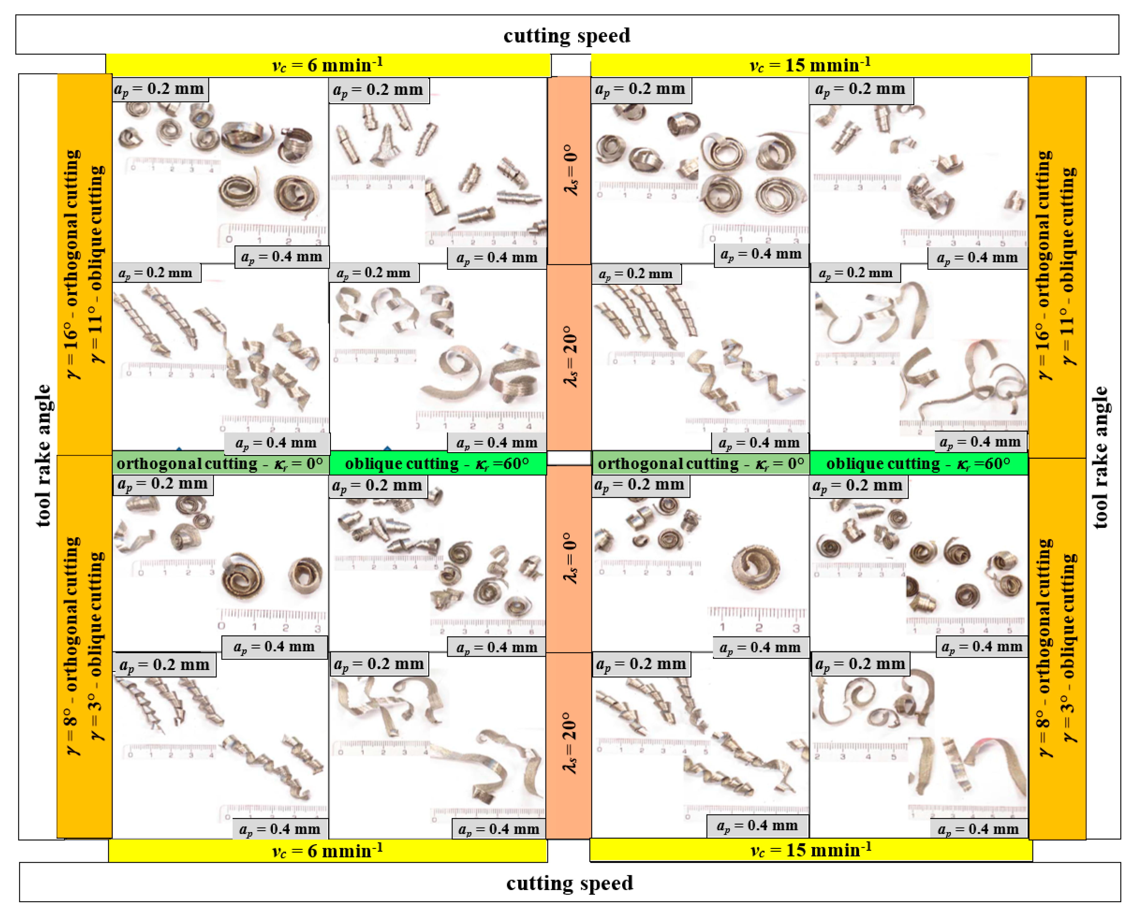
Within the experimental study, the variables according to

Table 4. The variables and ranges of individual values.

Variables		Symbols	−α	−1	0	+1	+α
Cutting speed (m·min−1)	vc	x1	6	8.25	10.5	12.75	15
Cutting depth (mm)	ap	x2	0.2	0.25	0.3	0.35	0.4
Angle of tool orthogonal rake—orthogonal cutting (°)	γ	x3	8	10	12	14	16
Angle of tool orthogonal rake—oblique cutting (°)	γ	(x3)	3	5	7	9	11
Angle of tool cutting edge inclination (°)	λs	x4	0	5	10	15	20

were taken into account, while the codes for the specific values of individual variables are referred in

Table 5. The codes for the specific values of individual variables.

Code	Specific Values of Variables
−α	xmin
−1	[(xmax + xmin)/2] − [(xmax − xmin)/2α2]
0	(xmax + xmin)/2
+1	[(xmax + xmin)/2] + [(xmax − xmin)/2α2]
+α	xmax

.

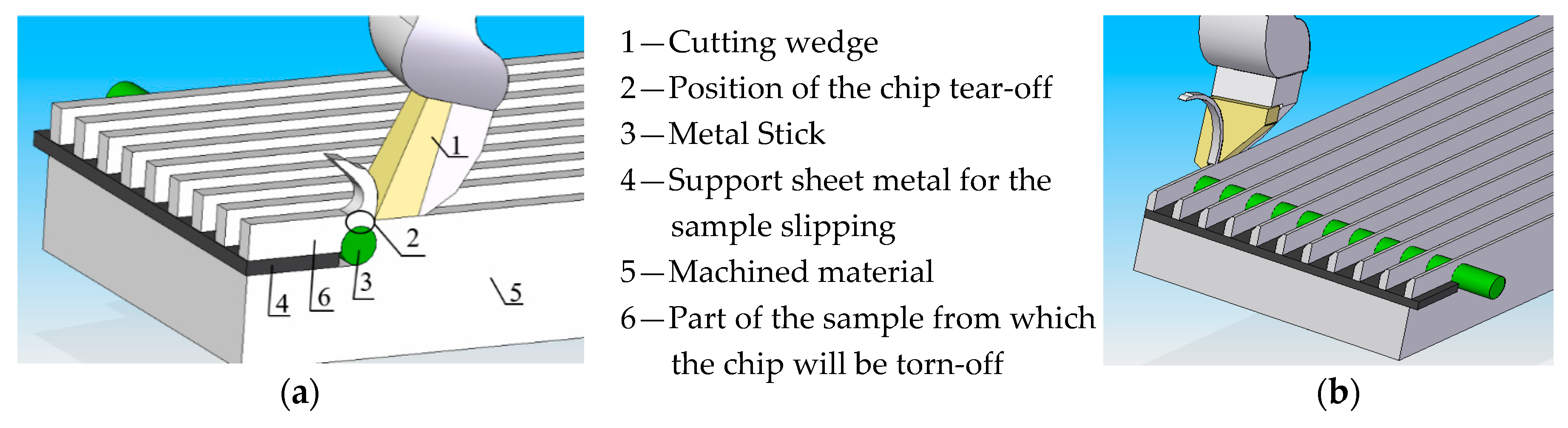
To track changes in the zone of chip forming, the machining process had to be stopped immediately, thus interrupting tool and workpiece contact. This is based on the observation of the chip end produced in interrupted cutting, e.g., in planing or face milling.

A reliable method to stop the machining process immediately was developed. Its principle lies in a chip root acquisition by modifying the end of the workpiece, according to Figure 6. The goal of the proposed method and the special workpiece design was to avoid deformation and a thermal influence of the material, which could cause changes in the microstructure of a material. Due to this reason, for all operations within the workpiece preparation, a cooling medium 5% emulsion from fully synthetic oil JCK PS (manufacturer JCK, Ltd., Prešov, Slovakia) was used.

At the point of departure of the tool “1” from the engagement, a groove was cut, where the sheet metal insert “4” was inserted to prevent deformation of the specimen during rupture. A hole of 8 mm diameter was drilled behind the groove, and a metal rod “3” was inserted therein, which prevented the hole from deforming. When the tool passed above the metal rod, the section “2” became narrower and the material ruptured, similar to in the tensile test. Sample “6” was rapidly thrown up in the direction of tool movement at a rate greater than cutting speed, and on the sample, the plastic deformation state corresponding to the actual cutting speed was captured.

The experiment was carried out on a planer without the use of cooling, since the cutting length of the tool path was about 200 mm, and thus the tool and workpiece were not overheated.

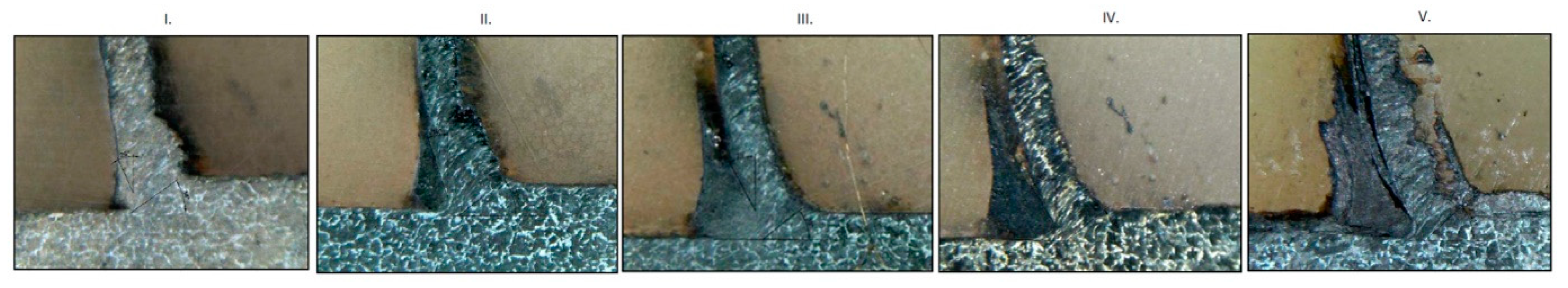
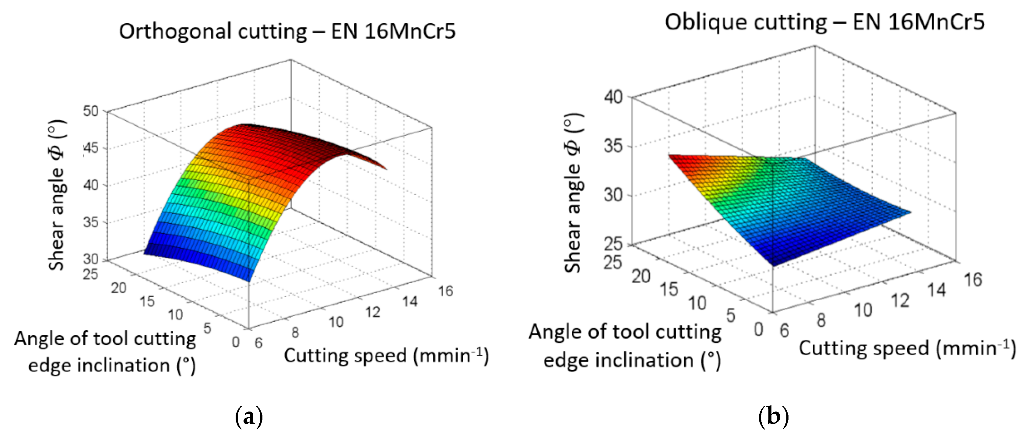
The shear angle Φ was measured at a chip root. The samples were ground five times, polished, and etched. Also, the shear angle, i.e., angle of the boundary between the deformed and undeformed material, and angle of built up edge were measured five times at each sample. An example of an investigated sample is presented in Figure 7.

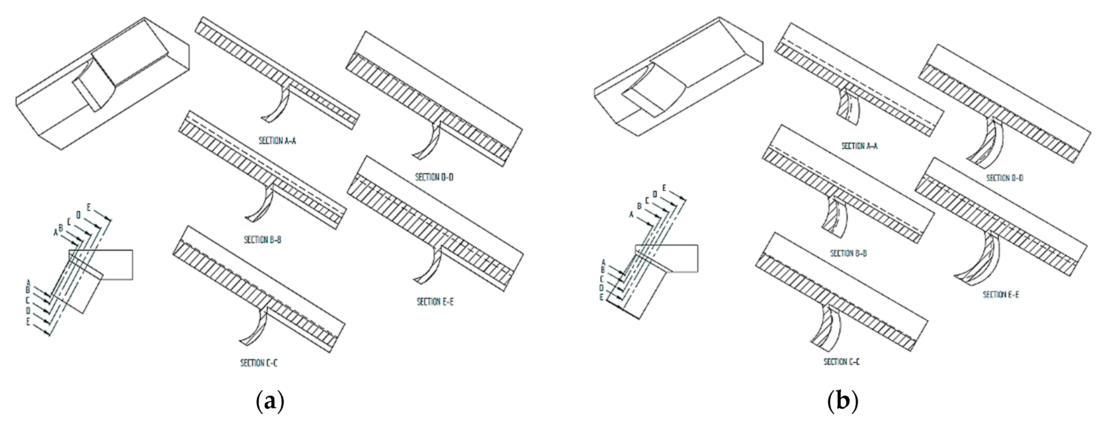
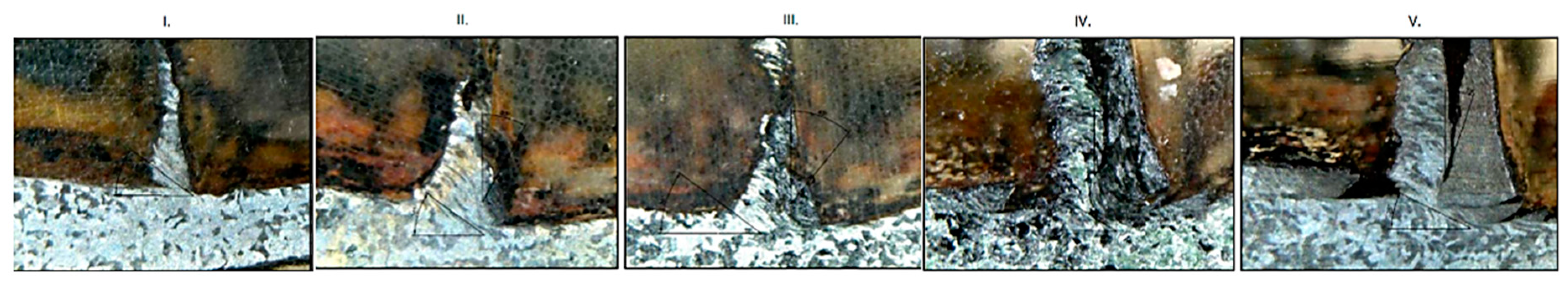
The angle of the tool cutting edge at orthogonal cutting was κ_r = 0° and at oblique cutting it was κ_r = 60°. At the same time, the angle of the tool of cutting edge inclination λ_s was also changed. Thus, it is very important to evaluate the shear angle correctly. Figure 8 shows a chip root sample, and shows how the change of the angle of main cutting edge inclination λ_s would affect the individual cross-sections of the sample.

It is not very difficult to solve the issue of orthogonal cutting. However, for oblique cutting, the angle of the tool main cutting edge κ_r and also the angle of the tool cutting edge inclination λ_s have to be taken into account. The figures below show the chip root sample and successive cross-sections of the sample at λ_s = 0° (Figure 9a) and λ_s > 0° (Figure 9b). This approach was also used for chip root evaluation within the research.

4. Results and Discussions

4.1. Types of Chips

4.1.1. A Chip Root of EN C45 Steel

For the orthogonal cutting of EN C45 steel, the sample at cutting speed v_c = 15 m·min⁻¹, depth of cut a_p = 0.2 mm, rake angle γ = 8°, and angle of main cutting edge inclination λ_s = 0°, was selected as a representative sample. Since it was orthogonal cutting, the tool cutting edge angle was κ_r = 0°. The views (magnified 200×) on an etched sample in all five cross-sections are in Figure 10.

In the first cross-section, the measured shear angle Φ was 34°. A second cut was made on the sample after the removal of an approximately 0.5 mm layer. The structure was more clearly visible due to better etching of the sample and the shear measured angle was Φ = 37°. This angle is 3° greater than on the first cut. The evaluation of the clearly observable built-up edge shows that the tool rake angle of 8° was increased to 19°. The created built-up edge on the tool assumed the function of the cutting tool, and thus it can be claimed that the rake angle increased significantly. At the third cut, it can be stated that the shear angle increased by 2° and at the same time the rake angle increased by the built-up edge of 20°, so the rake angle was 28°. On the fourth cut of the chip root sample, the shear angle was retained but an increase in the rake angle to 33° was observed through the built-up edge. On the built-up edge in the third cut, there was glued material, and the length of contact of the built-up edge and the outgoing chip was longer than that observed on the fourth cut. Based on this, it can be stated that the length of the contact of the tool face with the outgoing chip does not have to be the same over the entire width of the cut, and thus the friction coefficient will also be different. On the fifth cut of the chip root, the shear angle increased by 3° and, at the same time, the rake angle increased. At this cross-section, it was shown that the length of contact of the outgoing chip with the tool face, in this case through the face of the formed built-up edge, was not constant over the entire width of the cut. For this reason, the friction coefficient, which affects the heat generated in the cutting area, also changed.

As a representative sample for the chip root observation at the oblique slow-rate cutting of EN C45 steel, a sample obtained from machining with the following parameters was selected: v_c = 6 m·min⁻¹, a_p = 0.2 mm, γ = 3°, λ_s = 0°. Individual shapes of the chip roots, magnified 200×, are presented in Figure 11.

In the first cut, the measured shear angle Φ was 35°. In the second chip root cut, the shear angle was 4° less, so it was Φ = 31°. In both figures of the first and second chip root cross-section, there was no clearly noticeable built-up edge. The third cut showed an even smaller shear angle of Φ = 26° and at the same time, it can be stated that the rake angle was also reduced compared to the second cut. A slight increase in shear angle to 28° in the fourth chip root cut was caused by a slight increase in the rake angle. Similarly, in the fifth and final cut, an increase in shear angle to 32° was also observed. As mentioned above, the size of the shear angle is closely related to the size of the rake angle. The built-up edge directly on this sample was not clearly observable, but it occurred at the cutting edge of the tool in all cases of cutting.

Based on the shear angles measured in all five cross-sections, the average value was computed. The average values of the shear angles obtained by the machining of EN C45 steel with variable machining conditions, that were characterized by the matrix for statistical processing, are organized in

Table 6. Experimentally obtained values of temperature in cutting zone for orthogonal and oblique machining of EN C45 steel.

vc (m·min−1)	ap (mm)	γ (°)	λs (°)	Φ (°)
				Orthogonal Cutting	Oblique Cutting
−1	−1	−1	−1	39.8	30.4
+1	−1	−1	−1	38.8	32.4
−1	+1	−1	−1	42.0	33.6
+1	+1	−1	−1	40.6	37.2
−1	−1	+1	−1	36.6	39.0
+1	−1	+1	−1	42.2	32.0
−1	+1	+1	−1	40.2	34.0
+1	+1	+1	−1	42.0	37.8
−1	−1	−1	+1	35.0	31.4
+1	−1	−1	+1	36.4	45.6
−1	+1	−1	+1	42.4	26.6
+1	+1	−1	+1	37.8	30.2
−1	−1	+1	+1	37.8	34.0
+1	−1	+1	+1	39.8	45.0
−1	+1	+1	+1	40.4	35.6
+1	+1	+1	+1	39.0	34.6
−α	0	0	0	38.2	34.2
+α	0	0	0	29.8	39.8
0	−α	0	0	39.0	39.2
0	+α	0	0	38.0	33.8
0	0	−α	0	39.2	38.6
0	0	+α	0	38.2	42.6
0	0	0	−α	40.8	44.6
0	0	0	+α	40.8	37.8
0	0	0	0	38.0	27.6

.

The data were statistically processed and according to the Grubbs’ testing criterion [36], it could be stated that the measured values were not burdened by grave mistakes. The coefficients of regression functions were calculated using the software MATLAB 2016 and their significance was tested according to the Student’s criterion.

The regression functions (20) and (21) were built. According to the Fisher–Snedecor-tested criterion [38], they described the experiment adequately, while the reliability of the relationship was R² = 0.92 and 0.94, respectively:

(a)

For orthogonal cutting:

$$\begin{array}{c}y=-0.3947x_0+8.4952x_1+5.5938x_2-1.6685x_3+0.0176x_4-0.3475x_1{x}_2\\ +0.1452x_1{x}_3-0.0118x_1{x}_4-0.1465x_2{x}_3-4.5093x_1^2+4.6121x_2^2+0.9621x_3^2.\end{array}$$

(20)

(b)

For oblique cutting:

$$\begin{array}{c}y=1.5410x_0-0.6329x_1-3.5076x_2-1.7228x_3-0.2007x_4-0.2010x_1{x}_2\\ -0.2384x_1{x}_3+0.0361x_1{x}_4+0.1180x_2{x}_3-0.0771x_2{x}_4+0.0091x_3{x}_4+0.4437x_1^2\\ -3.1096x_2^2+1.3852x_3^2-0.0434x_4^2.\end{array}$$

(21)

Based on measured data, the dependencies of the shear angle Φ on the following combinations pairs of parameters were evaluated for both orthogonal and oblique cuttings:

• cutting speed v_c and cutting depth a_p;
• cutting speed v_c and rake angle γ;
• cutting speed v_c and the angle of tool cutting edge inclination λ_s;
• cutting depth a_p and rake angle γ;
• cutting depth a_p and the angle of tool cutting edge inclination λ_s;
• rake angle γ and the angle of tool cutting edge inclination λ_s.

The dependences were plotted and they are presented in Figure 12, Figure 13, Figure 14, Figure 15, Figure 16 and Figure 17.

For the orthogonal cutting of EN C45 carbon steel (Figure 12a), the cutting depth had a slightly more pronounced effect than the cutting speed, while for oblique cutting (Figure 12b), the cutting depth had a much more significant effect on the shear angle than the cutting speed. Maximum shear angle values were achieved at the maximum cutting depth for orthogonal cutting, and vice versa for oblique cutting at minimum cutting depth and higher cutting speeds.

The interaction of cutting speed and rake angle was totally opposite in both cutting methods. In orthogonal cutting (Figure 13a), the cutting speed had a more significant effect compared to the rake angle and the maximum shear angle values were reached at extreme rake angle and maximum cutting speed values. With respect to oblique cutting (Figure 13b), the effect of the rake angle was more pronounced than the effect of the cutting speed and the maximum shear angle values were reached at the minimum rake angle values.

The influence of the angle of tool cutting edge inclination on the change in shear angle compared to the cutting speed was not noticeable for orthogonal cutting (Figure 14a). For oblique cutting (Figure 14b), as was already mentioned above, the effect of the cutting speed was less significant, and therefore the effect of the angle of the tool cutting edge inclination on the shear angle change is also observable in the graph. For orthogonal cutting, maximum shear angle values were achieved at higher cutting speeds (from the used speed range), and within oblique cutting, they were achieved at minimum cutting speeds and minimum angles of the tool cutting edge inclination.

The depth of the cut layer had a significant influence on the shear angle for both types of machining. For orthogonal cutting (Figure 15a), the rake angle affected the change in shear angle slightly more than for oblique cutting (Figure 15b). For orthogonal cutting, the maximum values of the shear angle were achieved at the maximum values of the cutting depth, and for oblique cutting, maximum values of shear angle were observed at the maximum rake angle.

A common feature of both cutting methods, within the interactions of the parameters presented in Figure 16, was an invisible effect of the angle of the tool cutting edge inclination on the shear angle. As is clear from these graphs, the maximum shear angle values were achieved for orthogonal cutting at the maximum cutting depth and within oblique cutting at the minimum depth of cut.

The effect of the rake angle and the angle of the tool cutting edge inclination on the shear angle had the same character in both cutting methods (Figure 17). Maximum shear angle values were achieved at minimum rake angle values, and the lowest values of the shear angle Φ were achieved at mean rake angle values.

4.1.2. A Chip Root of EN 16MnCr5 Steel Observation

For the orthogonal cutting of EN 16MnCr5 steel, a chip root obtained in machining with the following cutting parameters was selected as a representative sample for observation: cutting speed v_c = 15 m·min⁻¹, cutting depth a_p = 0.4 mm, rake angle γ = 8°, and angle of the main cutting edge inclination λ_s = 0°. All five cross-sections of the chip root with magnification 200× are shown in Figure 18.

On the first cut of the sample, the shear angle was Φ = 31° and the rake angle of the formed built-up edge was 34°. On the second cut of the chip root, the shear angle increased by only one negligible degree and the rake angle of the formed built-up-edge remained unchanged at 34°. However, in this cross-section, the length of a contact surface between the built-up edge rake and the outgoing chip was several times greater than in the first section, resulting in a different coefficient of friction for both cases mentioned. In the third cut, a greater shear angle of Φ = 37° was measured, as well as a greater rake angle, until 44°. Again, the length of the contact between the outgoing chip and the built-up edge was different, and the stalled layers of hardened material were visible on the built-up edge. In some cases, the Vickers microhardness HV of the built-up edge was also measured at a load of 200 g in a duration of 10 s. While in the area of primary deformation the hardness was about 200 HV, in the built-up edge it was about 600 HV. The shear angle in the fourth section was 36°. The rake angle (of the built-up edge) was 33°, and the chip was adhered to the face of the tool built-up-edge, while the contact length between the face of the built-up edge and outgoing chip was greater compared to the third cut. In the fifth cut of the chip root of EN 16MnCr5 steel, the shear angle was the largest and the built-up edge appeared almost the same as in the fourth cut. The built-up edge on the cutting edge of the tool over the entire width of the cut significantly increased the rake angle, and thus influenced the shear angle in the individual cross-sections. At the same time, the built-up edge considerably increased the radius of the cutting edge round, indicating that the tool geometry was different during cutting than what was chosen to perform the experiment. An important element is the length of the contact surface between the face of the built-up edge and outgoing chip. It is shown in Figure 18 that the length of this contact surface was not constant over the entire width of the cut. Since the built-up edge was not stable, it could “tear-off” from the tool face and so change the shape of the tool during cutting, due to the same reason the rake angle cannot be considered constant even in the individual parts of the cutting width.

The sample obtained at oblique machining of EN 16MnCr5 steel with cutting parameters v_c = 15 m·min⁻¹, the cutting depth a_p = 0.4 mm, the rake angle γ = 3° and the angle of the main cutting edge inclination λ_s = 0°, was selected as the representative sample for a description. The chip-roots in cross-sections of this sample magnified 200× are presented in Figure 19.

On the first cut of the sample chip root, the built-up edge was not noticeable, but according to the shape of the outgoing chip, the rake angle appeared negative, while the rake angle of the straight roughing tool was positive, at γ = 3°. The cutting angle Φ was 36°. On the second cut, the built-up edge was already visible and the shear angle was reduced by 1° compared to its size on the first cut to 35°, which is a negligible change. On the third cut of the chip root, the rake angle increased and, at the same time, the shear angle slightly increased, to the value of 36°. The chip root in the fourth cut pointed to how the radius of the cutting edge round increased and, at the same time, the rake angle reduced. For this reason, the shear angle was also reduced to 29°. In the fifth cut, both the rake angle and the shear angle (Φ = 26°) were smaller. In this case, it can be seen how the machined surface was damaged by the build-up “tearing off”, which left from the cutting area.

The matrix of the experimental compositional plan for the evaluation of shear angle for the EN 16MnCr5 steel machining was designed in the same way as it was for EN C45 steel, for both cutting methods. The experimentally obtained values of the shear angle Φ, as well as the encoded matrix of individual cutting condition parameters, are shown in

Table 7. The measured shear angle values Φ for both orthogonal and oblique cutting of EN 16MnCr5 steel.

vc (m·min−1)	ap (mm)	γ (°)	λs (°)	Φ (°)
				Orthogonal Cutting	Oblique Cutting
−1	−1	−1	−1	43.0	35.4
+1	−1	−1	−1	39.2	42.8
−1	+1	−1	−1	35.6	24.2
+1	+1	−1	−1	35.4	31.4
−1	−1	+1	−1	37.2	30.8
+1	−1	+1	−1	38.2	33.8
−1	+1	+1	−1	42.2	31.8
+1	+1	+1	−1	39.0	41.2
−1	−1	−1	+1	37.4	41.0
+1	−1	−1	+1	37.8	34.4
−1	+1	−1	+1	40.4	41.2
+1	+1	−1	+1	39.6	34.6
-1	−1	+1	+1	35.8	37.6
+1	−1	+1	+1	41.6	35.6
−1	+1	+1	+1	38.2	38
+1	+1	+1	+1	35.2	34.4
−α	0	0	0	40.2	35.8
+α	0	0	0	33.8	40.4
0	−α	0	0	34.8	39.2
0	+α	0	0	38.4	37.2
0	0	−α	0	37.4	35
0	0	+α	0	36.4	41.6
0	0	0	−α	41.8	36.0
0	0	0	+α	32.4	39.8
0	0	0	0	33.2	42.4

.

Using the software MATLAB, the following regression functions, (22) and (23), were defined for both types of machining, while their reliabilities R² were 0.91 and 0.93, respectively:

(a)

for orthogonal cutting:

$$\begin{array}{c}y=2.7826x_0+1.1743x_1+4.7878x_2-0.7749x_3-0.1338x_4-0.2652x_1{x}_2\\ +0.0469x_1{x}_3+0.0088x_1{x}_4+0.1330x_2{x}_3+0.0130x_2{x}_4-0.0085x_3{x}_4-0.6994x_1^2\\ +4.2200x_2^2+0.5177x_3^2-0.0510x_4^2;\end{array}$$

(22)

(b)

for oblique machining:

$$\begin{array}{c}y=0.2562x_0+0.0132x_1-5.6702x_2-0.7684x_3+0.1414x_4+0.2051x_1{x}_2\\ +0.0752x_1{x}_3-0.0652x_1{x}_4+0.5759x_2{x}_3+0.0315x_2{x}_4-4.5505x_2^2+0.6638x_3^2\\ +0.0169x_4^2.\end{array}$$

(23)

For both types of machining, the simultaneous interaction of two of the four parameters (cutting depth a_p, cutting speed v_c, rake angle γ, and angle of tool cutting edge inclination λ_s) and their effect on the shear angle Φ was evaluated. The obtained dependencies are presented in Figure 20, Figure 21, Figure 22, Figure 23, Figure 24 and Figure 25.

For the planing of manganese chromium steel EN 16MnCr5, the cutting depth had a more pronounced effect than the cutting speed on the shear angle change within both cutting methods. In orthogonal cutting (Figure 20a) the maximum shear angle was reached at the maximum depth of cut and in oblique cutting (Figure 20b) at the minimum depth of cut.

The effect of cutting speed compared to the rake angle was more pronounced in orthogonal cutting (Figure 21a), where maximum shear angle values were achieved at a higher cutting speed and at the boundary rake angle values. In oblique cutting (Figure 21b), maximum values were reached at minimum rake angle values.

The graphs in Figure 22 show a demonstrable influence of the angle of the tool cutting edge inclination on the change of shear angle compared to the cutting speed. In orthogonal cutting (Figure 22a), the cutting speed had a greater impact, but in oblique cutting (Figure 22b), the angle of tool cutting edge inclination had a more pronounced effect. In orthogonal cutting, the maximum shear angle values were achieved at a minimum angle of tool cutting edge inclination and at higher cutting speed values. In oblique cutting, maximum shear angle values were visible at a minimum cutting speed and maximum angle of tool cutting edge inclination.

Compared to cutting depth, the rake angle had only a slight effect on changes in the shear angle within both types of machining (Figure 23). The influence of cutting depth on the shear angle values have already been mentioned above. The angle of the tool cutting edge inclination (Figure 24) had a very similar slight effect to the rake angle in Figure 23, so the dependencies were almost of the same character.

The interaction of the shear angle with both the cutting edge inclination and rake angle is presented in Figure 25. It can be observed from the graphs that the dependencies had a similar character for both types of machining, while the angle of tool cutting edge inclination had an only slight effect on the shear angle compared to the rake angle. The minimal values were achieved at the mean values of the rake angle.

4.1.3. Comparison of the Chips of EN C45 and EN 16MnCr5 Steels

A comparison of some of the chip roots made from both types of investigated steel, i.e., EN C45 and EN 16MnCr5, is presented in

Table 8. Comparison of chip roots of EN C45 and EN 16MnCr5 steels with the same cutting parameters.

Type	EN C45	EN 16MnCr5
Orthogonal Cutting
	vc = 6 m·min−1; ap = 0.4 mm; γ = 16°; λs = 0°
	vc = 8.25 m·min−1; ap = 0.3 mm; γ = 12°; λs = 10°
	vc = 10.5 m·min−1; ap = 0.3 mm; γ = 12°; λs = 15°
	vc = 12.75 m·min−1; ap = 0.3 mm; γ = 12°; λs = 10°
	vc = 15 m·min−1; ap = 0.4 mm; γ = 8°; λs = 20°
Oblique Cutting
	vc = 6 m·min−11; ap = 0.4 mm; γ = 11°; λs = 0°
	vc = 8.25 m·min−1; ap = 0.3 mm; γ = 7°; λs = 10°
	vc = 10.5 m·min−1; ap = 0.3 mm; γ = 7°; λs = 15°
	vc = 12.75 m·min−1; ap = 0.3 mm; γ = 7°; λs = 10°
	vc = 15 m·min−1; ap = 0.4 mm; γ = 3°; λs = 0°

. All chips were formed by machining procedures, with the same cutting parameters obtained for orthogonal and oblique cutting. It can be seen that the behavior of the chip formation strongly depended not only on the materials but also on the cutting conditions.

Except for the input value of the tool orthogonal rake, the formed built-up edge influenced also the shear angle and the shrinkage factor K, along with the segment ratio r_c. These can be calculated with Equations (24) and (25), where h_c is the chip width, a_p is cutting depth, γ is the tool rake angle, and Φ is the shear angle [4,45,46]:

$$K=\frac{h_c}{a_p}= \frac{\cos \left(\varphi -\gamma \right)}{\sin \varphi };$$

(24)

$$r_c=\frac{1}{K} .$$

(25)

The values of the shrinkage factor K achieved within the experimental study are organized in

Table 9. Shrinkage factor K achieved within the experimental study.

Type of Steel	Type of Cutting	Shear Angle Φ (°)	Shrinkage Factor K
EN C45	Orthogonal cutting	29.8	1.92
		42.4	1.22
	Oblique cutting	26.6	2.05
		39.8	1.31
EN 16MnCr5	Orthogonal cutting	31.7	1.75
		42.2	1.3
	Oblique cutting	30.2	1.77
		42.4	1.21

.

All these real cutting parameters that entered into the machining process influenced the chip forming during machining. The summary overview of the effects of these parameters on the chip shapes is graphically presented in Figure 26 and Figure 27.

In the slow-rate machining of both steels, a shorter chip was created at a zero angle of inclination of main cutting edge when compared with the angle of inclination of the main cutting edge of 20°. At the same time, at a 20° angle of inclination of the cutting edge, a chamfer was formed along the edges of the chip, which corresponded to the angle of inclination of the main cutting edge and, thus, the chip was compressed in the direction of λ_s inclination and acquired the character of a spiral chip. In orthogonal cutting, at which κ_r = 0° and λ_s = 0°, a spiral flat chip was formed, which in some cases passed into a spiral conical chip. For κ_r = 0° and λ_s = 20°, a conical–helical long chip was constituted. In oblique cutting, where κ_r = 60° and λ_s = 0°, a conical–helical short chip was generated. At κ_r = 60° and λ_s = 20°, the chip shape changed to a coiled chip, while at rake angle γ_o = 11°, it was a tubular coiled chip and at γ_o = 3° it was a strip coiled chip.

5. Conclusions

Within the presented study, the shear angle for orthogonal and oblique slow rate machining was evaluated, depending on selected cutting parameters—cutting speed v_c; cutting depth a_p; rake angle γ; angle of tool cutting edge inclination λ_s—and the chip roots were observed, focusing on the formed built-up edge.

To evaluate the interaction of the parameters correctly, the compositional planned experiment was designed and a new reliable method for the chip root obtaining was developed. Experimentally obtained data were statistically processed, while the regression functions for both types of machining and for both steel types were defined and the dependencies of the selected parameters on the shear angle were plotted.

Based on the shear angle measurements, the individual dependencies were determined and the significance of the influences of the individual factors was evaluated. In both cutting methods, the cutting depth proved itself to be the parameter with the most significant influence on the shear angle change. For orthogonal cutting, the cutting speed was the second most significant parameter, and the rake angle was the third while for oblique cutting, the rake angle was the second and the tool cutting edge inclination angle was placed third. Maximum shear angle values were measured on the chip samples obtained in the orthogonal cutting of both steel types when the cutting speed and cutting depth were maximal and the rake angle was minimal. In the oblique cutting of both materials, this was at minimum values of the cutting speed, the cutting depth, and the rake angle.

In the preliminary research of the authors [13], where the changes in temperature and microhardness of a chip root were evaluated, the angle of tool cutting edge inclination appeared to be an insignificant parameter. However, regarding changes in the chip shape, the angles of tool cutting edge inclination λ_s and tool cutting edge κ_r were the most important parameters.

A major problem with respect to the accuracy and reproducibility of the experiment results was the build-up on the tool rake. This built-up edge increased the tool rake angle by 30° and, due to this, it adheres to the face of tool and it assumes the function of the tool. When measuring the rake angle on successive cuts of the chip root samples, the built-up edge was observed on every sample. Along with the shear angle, the size of the newly originated rake angle was observed. As the rake angle increased, the shear angle also increased, causing a more favorable shear direction in the plastic zone, and thus the chip formation process became simpler [47]. It is disturbing that the build-up edge was unstable and, as has been proven by the chip root cuts, the shape of the build-up edge and its influence on the tool geometry was not constant over the entire width of the cut. Also, the length of the contact face (taken at the moment as the tool face) with the outgoing chip was not constant over the entire cutting width. Consequently, there was a clear change in the friction coefficient in the contact region of the face and the outgoing material, and thus there is a presumption that there is an indirect dependence between the formation of the built-up edge or its adherence to the outgoing material and between the temperature generated in the cutting area by changing the friction coefficient.