Article

Experimental Determination of Electronic Density and Temperature in Water-Confined Plasmas Generated by Laser Shock Processing

by
Cristóbal Colón
1,*,
María Isabel de Andrés-García
1,
Cristina Moreno-Díaz
1,
Aurelia Alonso-Medina
1,
Juan Antonio Porro
2,
Ignacio Angulo
2 and
José Luis Ocaña
2
1
Department of Applied Physics, ETSIDI, Universidad Politécnica de Madrid, Ronda de Valencia 3, 28012 Madrid, Spain
2
Department of Applied Physics, ETSII, Universidad Politécnica de Madrid, José Gutiérrez Abascal 2, 28006 Madrid, Spain
*
Author to whom correspondence should be addressed.
Metals 2019, 9(7), 808; https://doi.org/10.3390/met9070808
Submission received: 17 June 2019 / Revised: 9 July 2019 / Accepted: 19 July 2019 / Published: 22 July 2019
(This article belongs to the Special Issue Laser Shock Processing and Related Phenomena)

Abstract

:
In this work, diagnoses of laser-induced plasmas were performed in several Laser Shock Processing (LSP) experiments using the Balmer Hα-line (656.27 nm) and several Mg II spectral lines. A Q-switched laser of Nd:YAG was focused on aluminum samples (Al2024-T351) in LSP experiments. Two methods were used to diagnose the plasma. The first method, which required two different experiments, was the standard for establishing the electronic temperature through the use of a Boltzmann Plot with spectral lines of Mg II and self-absorption correction. The Stark width of the Balmer Hα-line was used to determine the electron density in each of the cases studied. The second method had lower accuracy, but only required an experimental determination. Two parameters, the electronic temperature and the electron density, were obtained with the aid of the Hα-line in a single data acquisition process. The order of magnitude of the temperature obtained from this last method was sufficiently close to the value obtained by the standard method (within a factor lower than 2.0), which is considered to be important in order to allow for its possible use in industrial conditions.

1. Introduction

Laser Shock Processing (LSP) is based on focusing a pulse of a high energy laser (I > 109 W/cm2, τ < 50 ns) over a piece of metal. It results in the instantaneous vaporization of the piece’s surface and the generation of a high temperature and density plasma composed of the different ionized species of elements present in the piece and in the atmosphere. The high pressure of the plasma generates a shock wave that propagates to the piece, which affects its mechanical characteristics. Today, LSP is a consolidated alternative for improving the surface properties of metal alloys. This technique has been studied since the 1960s, when Askar’yan and Moroz [1] discovered that a high-energy laser pulse produces backpressures in the surface of the metal material on which the laser is focused (target). In Fairand et al. [2] it was found that laser shocking induced a tangled dislocation substructure similar to explosively shocked aluminum. The stress waves were studied using the piezoelectric response of X-cut quartz-crystal disks by Yang [3]. Since then, numerous works have aimed at finding the best conditions in which the technique should be applied. In 1990, Fabbro et al. [4] quantitatively described the evolution of the plasma in a LSP experiment under confined geometry using different characteristic plasma-dynamics stages, including plasma pressure buildup, plasma development under the laser irradiation, and final plasma expansion until the pressure decreases and it is too low to cause plastic deformation in the material. An explanation of this phenomenon was given by Berthe et al. [5].
In 1997, Sano et al. [6] confirmed that the underwater shock processing with YAG was feasible to improve residual stress in metal. There are different studies about several methods to confine the plasma (see, e.g., Morales et al. 2009 [7]), indicating the crucial role of a plasma-confining layer in withstanding both the laser irradiation (with minimum internal breakdown) and the plasma pressure needed to transmit to the shocked target. The use of glass or quartz plates as confining layers are theoretically very suitable, but are generally only valid for a few laser shots and in measurements made in the laboratory, which are far from the needs imposed by industrial application of the technique, so purified water is normally used as the LSP confining medium.
The observation of the plasma shock wave through the confining medium has always been a subject of much interest in order to characterize the actual impulsion transmitted to the shocked material, a key point regarding the systematic monitoring and control of LSP processes in an industrial environment (see, e.g., Berthe et al. [5] and Ocaña et al [8]).
In 2009, Martí-Lopez et al. [9] performed interferometric measurements in order to record hemispherical shock fronts, cylindrical shock fronts, plane shock fronts, cavitation bubbles, and phase disturbance tracks. A summary of the different results obtained in the LSP experiments are presented by Ocaña et al. [8] along with some conclusions about the LSP technology as a profitable industrial method.
Recently, works on the effect of the LSP process have also been presented by some of the authors of this study. A comparison between experimental values and numerical predictions of the inside propagation of the residual stresses in plates of Al2024-T351 of 2 mm thickness was presented in 2015 by Ocaña et al. [10]. Also in 2015, a study on the influence of the randomness of the superposition of pulses on the final anisotropy of the residual stresses induced in the treated material was completed by Correa et al. [11].
Several theoretical works try to model the LSP process with the purpose of finding the practical criteria for its optimization. A self-closed thermal model for LSP was described by Wu and Shin [12]. Unlike most of the existing laser peening models, there are no free parameters in this model, and all the variables are calculated based on related physics theories. Later, a model-based systematization of process-optimization criteria and a practical assessment on the real possibilities of the technique along with practical results at a laboratory scale on the application of LSP to characteristic high-elastic limit metallic alloys were presented in 2008 by Morales et al. [13]. A calculation model conceived for the analysis of the problem of laser shock wave generation and propagation was presented in 2013 by Ocaña et al. [14]. However, these works were not able to predict the best conditions of application of the LSP technique with changes in the target materials. This is due in part to the large number of physical processes involved. As an example, although these models provide, as indicated, good predictions about the shock wave on the surface of the sample, their forecasts on the parameters of the plasma are too far from the experimental values, even when the plasma is confined in air. There is no experimental information on these properties in the case of plasma that is confined by water in flow.
The presence of hydrogen in the plasma is proof that chemical attacks on the surface of the sample can occur during the process. The interaction between the laser, the plasma, and the surface of the sample goes beyond the mechanical impact of the shock wave on the target. The relative presence of different ions in the plasma and its chemical interaction with the surface cannot be established without the knowledge of the plasma electron density number and its electronic temperature.
The purpose of this work was to experimentally estimate, by means of a practical (ideally industrially applicable) procedure, the electron density and the electronic temperature of the plasma in water-flow conditions to study chemical interactions between plasma and the surface of the sample and improve the theoretical treatments of the LSP process.
These studies of electron density number and plasma temperature determination have been performed for years using the technique known as Laser Induced Breakdown Spectroscopy (LIBS). The LIBS technique is based on the study of the emission of the different atomic and ionic species present in plasma. An excellent compilation of experiments and applications of the LIBS technique can be found in the literature (see, e.g., Musazzi and Perini [15]). This technique has been used in several scientific applications by the authors signing this work. In 2006, Colón and Alonso-Medina [16] measured Stark broadening of several Pb II spectral lines, and in 2011, Alonso-Medina [17] measured the broadening Stark of Pb III spectral lines. The LIBS technique also stands out as an analytical technique in different industrial applications (see, e.g., Noll et al. [18]).
In 2006, El Sherbini et al. [19] used the Hα-line to measure electron density in an experiment of the laser-induced breakdown of plasma in air. In 2010, Parigger and Oks [20] presented a review about plasma diagnostics based on Stark broadening of hydrogen Balmer lines in laser-induced breakdown of plasma. Later, in 2012, the Hα-line was used again by El Sherbini et al. [21] to determine the electron density in aluminum plasma and to correct the self-absorption in the Mg I and Mg II spectral lines present in this plasma. In 2004, De Giacomo et al. [22] completed several experiments of laser induced breakdown spectroscopy in aqueous solution. Nath and Khare [23] studied laser-induced breakdown experiments in water in 2010 using the emission bands of different molecular species.
As mentioned in a previous work by Moreno-Díaz et al. [24], the flow of water in LSP conditions weakens the emission of all species present in the plasma, with some exceptions. In the present work, in addition to the emission of hydrogen, already mentioned above, a weak emission of Mg II in the 279.5 nm zone was targeted. As in the previous work, the electron density was measured using the Stark width of the Hα-line. Now, the temperature can be estimated directly under LSP conditions using the emission of the spectral lines of Mg II.
The current work used the Stark width of the Hα-line on a sample of aluminum alloy (Al2024-T351) in LSP conditions (with water as the confining environment). The novelty of this study is in the measurement of the electronic temperature, which was performed directly in the LSP experiments using a Boltzmann plot with measurements of the intensities of the spectral lines of species present in the plasma in the water flow, not in air as was used in the earlier work of Moreno-Diaz et al. [24]. Measurements were taken with different delay times from the laser pulse (2–5 µs), while the plasma cooled adiabatically, allowing us to obtain the width and shift of the Hα-line in all cases. In order to obtain the best conditions for measurements, different gate times of 100 ns, 200 ns, 300 ns, 500 ns, and 1000 ns were used.
In order to verify the suitability of the proposed one-determination diagnosis procedure, a comparison of the obtained temperatures with those estimated from the shift of the Hα-line (two determinations needed) was successfully performed. This diagnosis with a single experiment would allow for the much-needed real-time monitoring of plasma behavior as described in Ocaña et al. [25] and Takata et al. [26].
In this paper, in Section 2 (Materials and Methods) the equipment and the experimental procedures are described. In Section 3 (Results) the analysis of the results is presented by comparing the values of the plasma temperature achieved by two different methods. Finally, in the Section 4 and Section 5 (Discussions and Conclusions, respectively) we present the possibilities of plasma diagnosis through a single experiment and through a second experiment without using the Mg II lines.

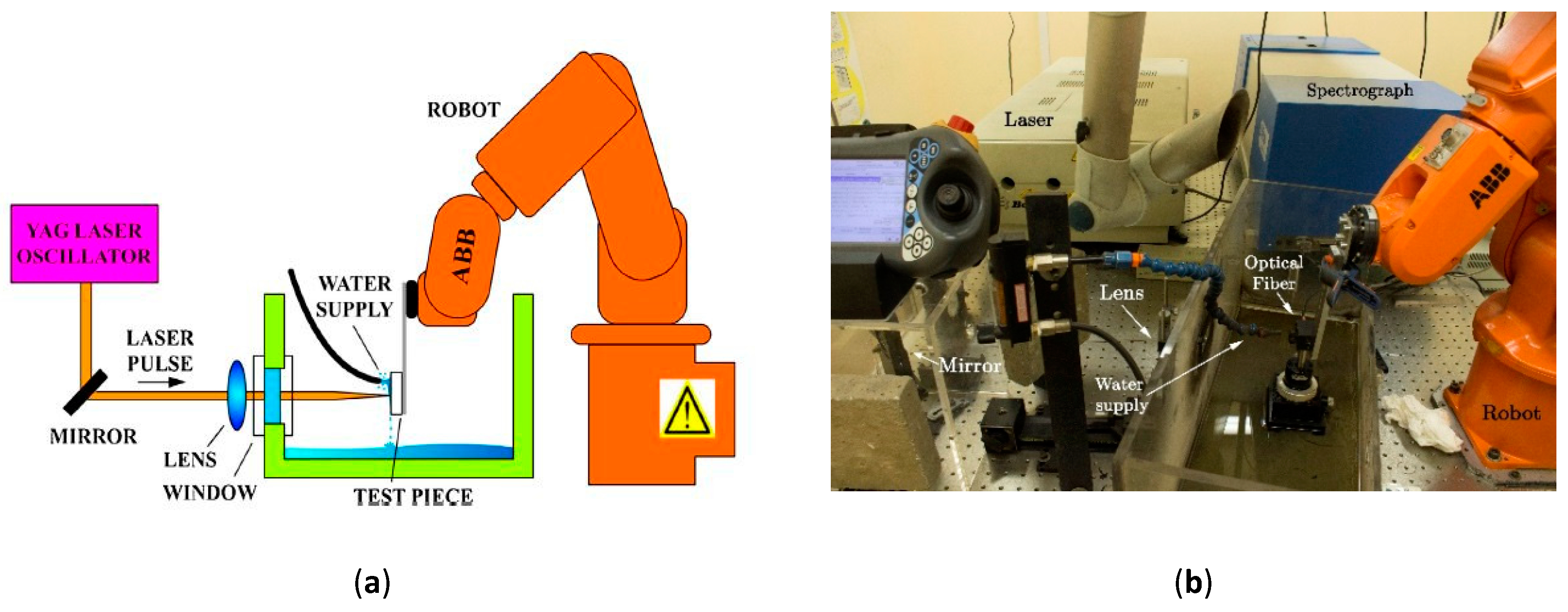
2. Materials and Methods

The experimental setup used in this work is the same as that used by the authors in a previous work (Moreno-Diaz et al. [24]). A schematic diagram of the experimental set-up is shown in Figure 1a,b.
A laser pulse of a Q-switched Nd:YAG laser (of 10 ns, 1.06 µm of wavelength, and 2.5 J per pulse) was focused using a 20 cm focal lens on a sample of certified aluminum alloy (Al2024-T351). The composition of the sample included in addition to aluminum around 4% Cu, 1.5% Mg, and 0.6% Mn. As can be observed in Figure 1, a constant water flux was supplied in this experiment. A typical crater, see Figure 2, of ~2 mm diameter was produced in the sample surface after the laser pulse. The image was obtained with a confocal microscope (LEICA DCM 3D´Leica Microsistemas S.L.U., L’Hospitalet de Llobregat, Spain). The irradiance of laser was approximately 10 GW/cm2.
The plasma light was collected by an optical fiber and directed to the spectrograph provided with a diffraction grating of 1800 grooves/mm. The placement of a lens to collect more plasma light may be an alternative in air, but the lens has been shown to be badly damaged by water splashes in the laboratory and probably would be even more so in an industrial environment.
Emission spectra were acquired using a spectrograph (Horiba Jobin Ybon FHR1000, HORIBA UK Limited, Northampton, United Kingdom) equipped with an ICCD camera (Andor, model iStar 334T, Oxford Instruments, Concord, MN, USA).
Measurements were taken 2 mm from the target surface (where the signal/noise ratio was the best). As we mentioned in our previous work, in spite of our attempts, the quality of the signal prevented us from making the Abel inversion, and so our data are spatially integrated and present the temporary integration of the measurement gate time.
A low-pressure Ne lamp (Oriel 6032, Newport, Irvine, CA, USA) was used to calibrate the wavelength scale. The instrumental profiles in the interest range were measured with a He-Ne laser, checking its full width at half maximum. The instrumental bandwidths in this range were found on average to be 0.18 ± 0.01 Å. In this bandwidth, it was found by numerical adjustment that the Lorentzian contribution was practically null.
Relevant LSP experiments were performed both under air and water confinement. Under air-confinement conditions, the composition of the plasma reflected the composition of the sample, obtaining spectral lines of Al I and Al II, Mg I and Mg II, Cu I and Cu II, and Mn I and Mn II, in addition to the Hα-line of the hydrogen, which can only be due to very weak traces of hydrogen in the plasma and a possible reaction between the ionized aluminum and the residual humidity of the air [21]. The presence of the water flow weakened the emissions of spectral lines differently than it did those of the Hα-line, which had a similar profile in air and in water flow in all cases. This effect can be observed in Figure 3.
As the profiles and the displacement of the Hα-line were practically identical under air and water flow confinement (LSP condition), the hypothesis of the similarity of the plasma behavior and properties under both conditions (already recognized in the previous work [24]) is considered sound.
In Figure 4a–c, images of the plasma trace at 2.5, 4, and 5 µs after laser pulse (gate time of 300 ns in all cases) and the corresponding spectra can be observed. As previously indicated, the presence of neutral hydrogen, although important for the obtained results, is residual, and confirms the practical non-absorption of the Hα line. The hostile conditions in which these measures must be carried out, with water in flow and splashing, makes it very difficult to experimentally contrast this claim. Nevertheless, the Hα lines did not show any self-absorption signs. In other words, there is full symmetry and no anomalous dip in the center. These facts have already been mentioned by El Sherbini et al. [19,21] in the electron density range of these kinds of experiments (described in Moreno-Diaz et al. [24]). Another relevant feature was the appearance of a red shift of the peak of the Hα-line which, in turn, was observed to decrease with the delay time.
In order to perform the analysis of the spectral lines, the obtained experimental profiles were adjusted to Voigt profiles generated numerically. To obtain the Lorentz experimental broadening of the line, the contribution of the instrumental profile was discounted.
Unlike the Lorentzian contribution, which was practically null, the Gaussian contribution of the instrumental profile of the used experimental device was important in relation to the Gaussian contribution found in the Voigt profiles of the Hα-line analyzed in this work. This fact advises against the use of this contribution to estimate the temperature of thermal agitation of hydrogen, which only in conditions of full thermodynamic equilibrium would coincide with the sought electronic temperature.
Figure 5 shows four examples of the fitting from a Voigt profile to experimental line emissions of the plasma. The Hα-lines corresponding to 4 µs delay time and gate times (emission integration times) of 100 ns, 300 ns, 500 ns, and 1000 ns are presented.
The corresponding Stark broadening and red shift appear in the left side of every spectrum. As can be observed, the best line profiles are at 300 and 500 ns. At 100 ns and 1000 ns there are slight asymmetries that are attributed to the fact that signal integration times are not adequate. At 100 ns, the signal integration time is too short and at 1000 ns, it is too long. It is also observed that despite these disadvantages for the 100 ns and 1000 ns gate times, the Stark widths and shifts obtained are the same in all gates within the experimental error margins.

3. Results

Plasma emission spectra in the range of 652.0–659.0 nm at different times after the laser pulse (2–5 µs) and with several gate times (100, 200, 300, 500, and 1000 ns) were obtained. The spectra were measured in LSP conditions (flow water over the sample). The main feature of the spectrum was the appearance of the Hα-line emission. In contrast to the spectrum obtained in air, in this case and as was observed in our previous work (Moreno-Diaz et al., [24]), the second order line of 327.39 nm Cu I does not appear.
The results obtained about Stark width and red shift after the fitting processes of the experimental data are presented in Table 1. In the first column the delays are presented, and in the successive columns, for each gate time, the corresponding Stark width and shift are shown. In these data, Δλ1/2 (Å) and d (Å) represent the Lorentzian component (in Å) of the Voigt profile (once the instrumental contribution had been discounted) and the Stark red shift, respectively.
The experimental red shifts obtained in this work were affected by a general uncertainty of around 15%, except for those that appear in parentheses (with time gates of 100 ns and 200 ns and for which the statistics of the data are poor, and the uncertainty may be higher). However, they are included in the table since they seem to indicate the experimental trend indicated by Griem [27]. The 100 ns and 200 ns time gates appear to have light-integration times that are too short. These low statistics are the reason why the use of short gate times for measurements in industrial conditions are discouraged.
An example of these results can be observed in Figure 6, where the displacement of the maximum emission of the Hα-line can be clearly appreciated.

3.1. First Method

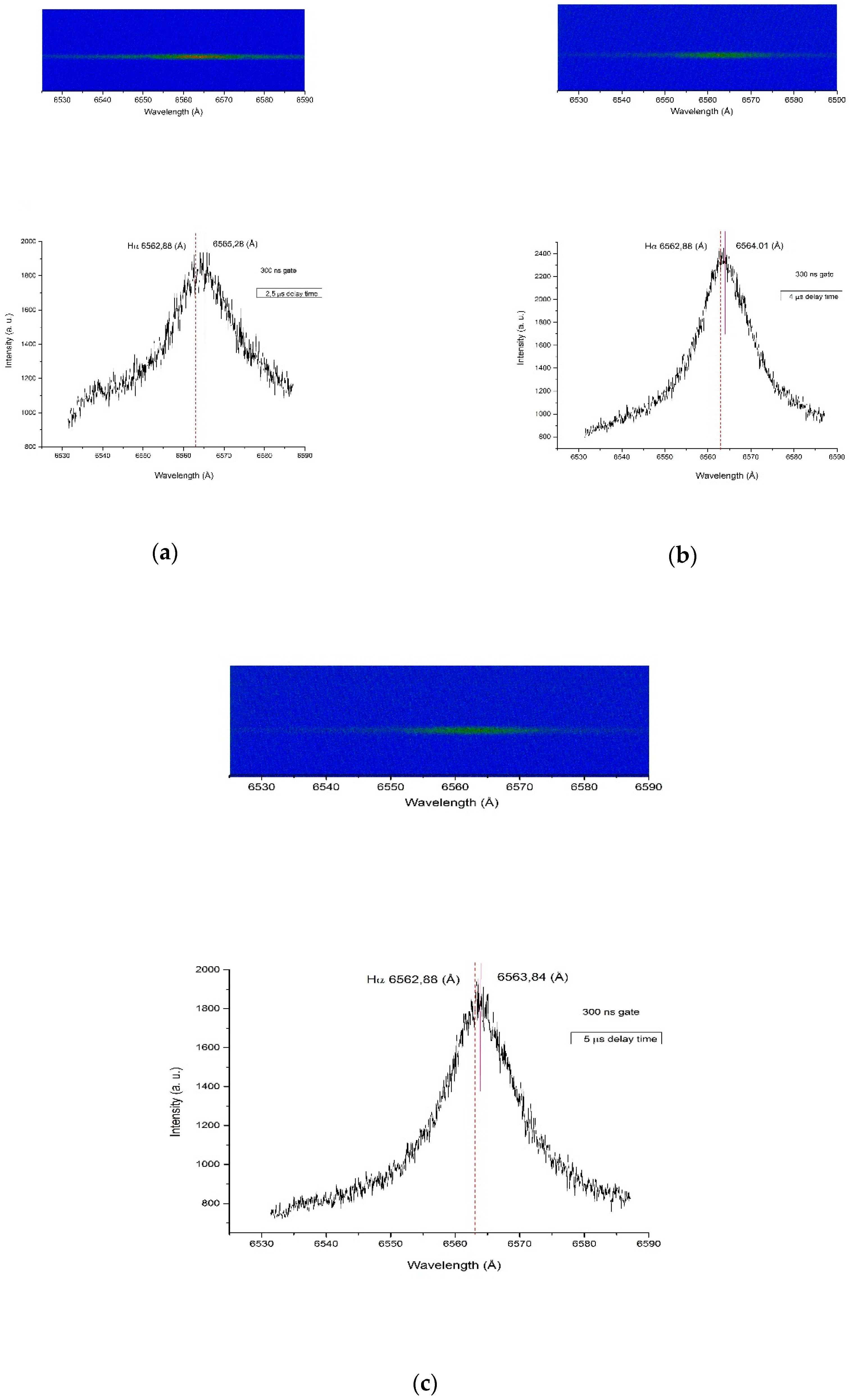
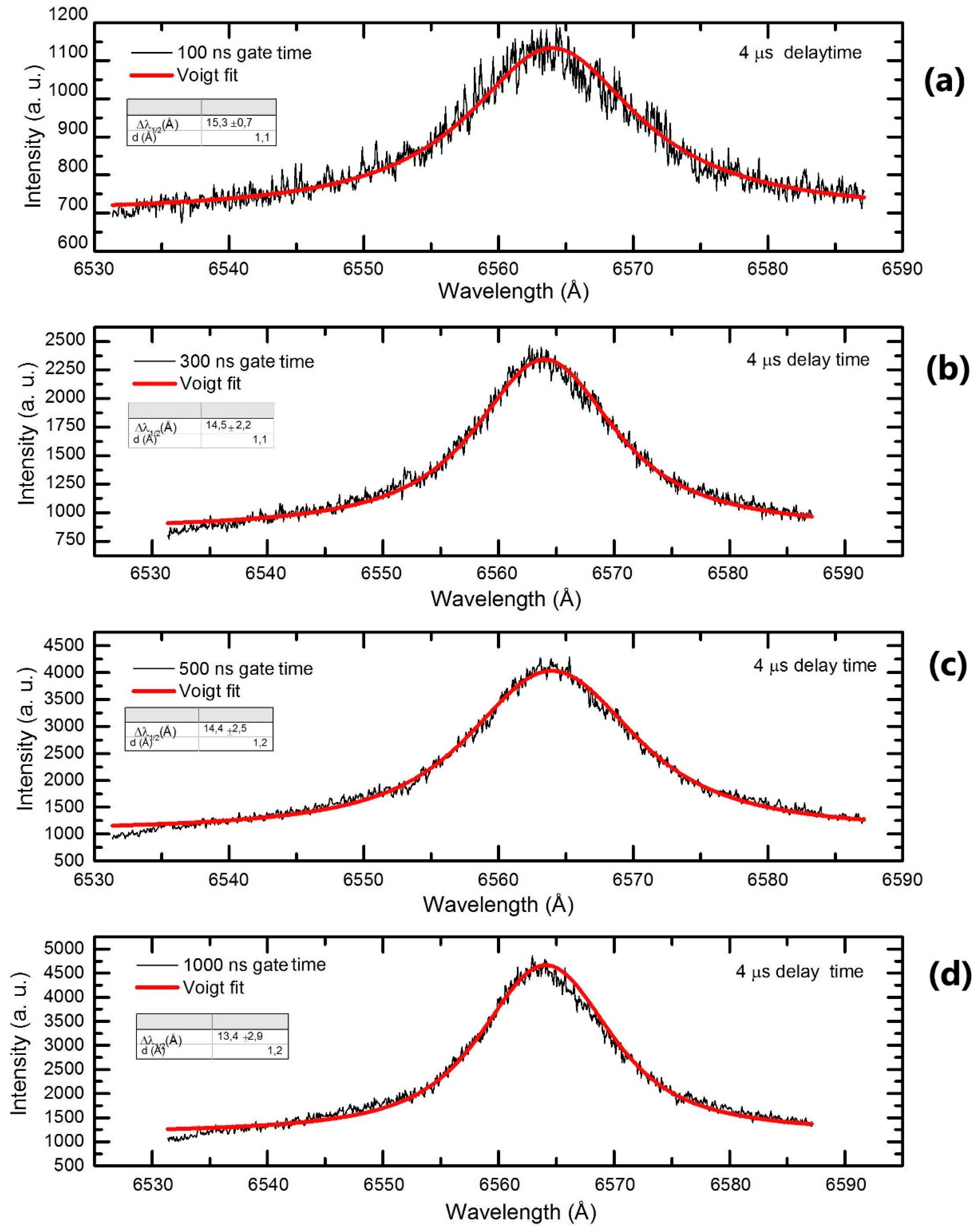
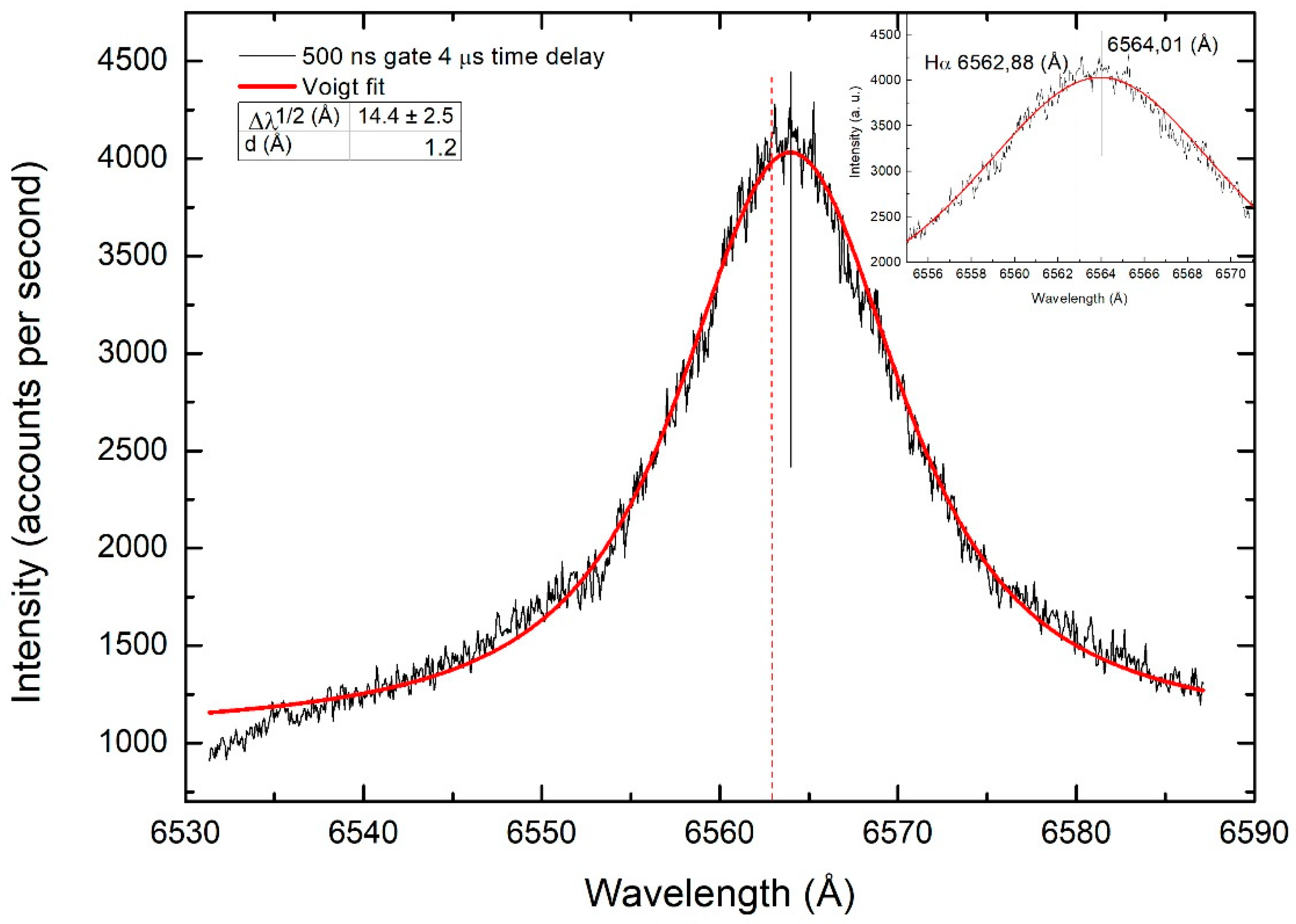
3.1.1. Electron Densities Determination

The following expression (given by Ashkenazy et al. [28]) was used to obtain the electron number density, Ne, from the width of the Hα-line:
Ne = 8.02 × 10¹²λ1/2/α1/2)3/2 cm−3
where α1/2 is half the width of the reduced Stark profiles in Å. Values of α1/2 for the Balmer series can be found in Griem [29] and also in Kepple and Griem [30].
In these references [29,30], it can be observed that the parameter α1/2 depends on the electron density and that it also varies slowly with the temperature, T (around 6% at 10,000 K). It is well known that for plasmas in air, in experimental conditions analog to those in this work, temperature will be between 10,000 and 15,000 K (El Sherbini et al. [19]; De Giacomo et al. [22]). In this work, as the profile of the Hα-line in air and in the LSP conditions were similar we used the parameter given by Griem at a temperature of 15,000 K. This assumption is justified in the next paragraph.
The values of the electron density obtained by this procedure are shown in Table 2 and were obtained using a value of α1/2 for an electron density of 1017 cm−3. Subsequently, an iterative method was used until the used parameters corresponded to the electron densities obtained. The uncertainties of the central values included the deviations in the Stark broadening, shown in Table 1, plus 6% due to temperature uncertainty.

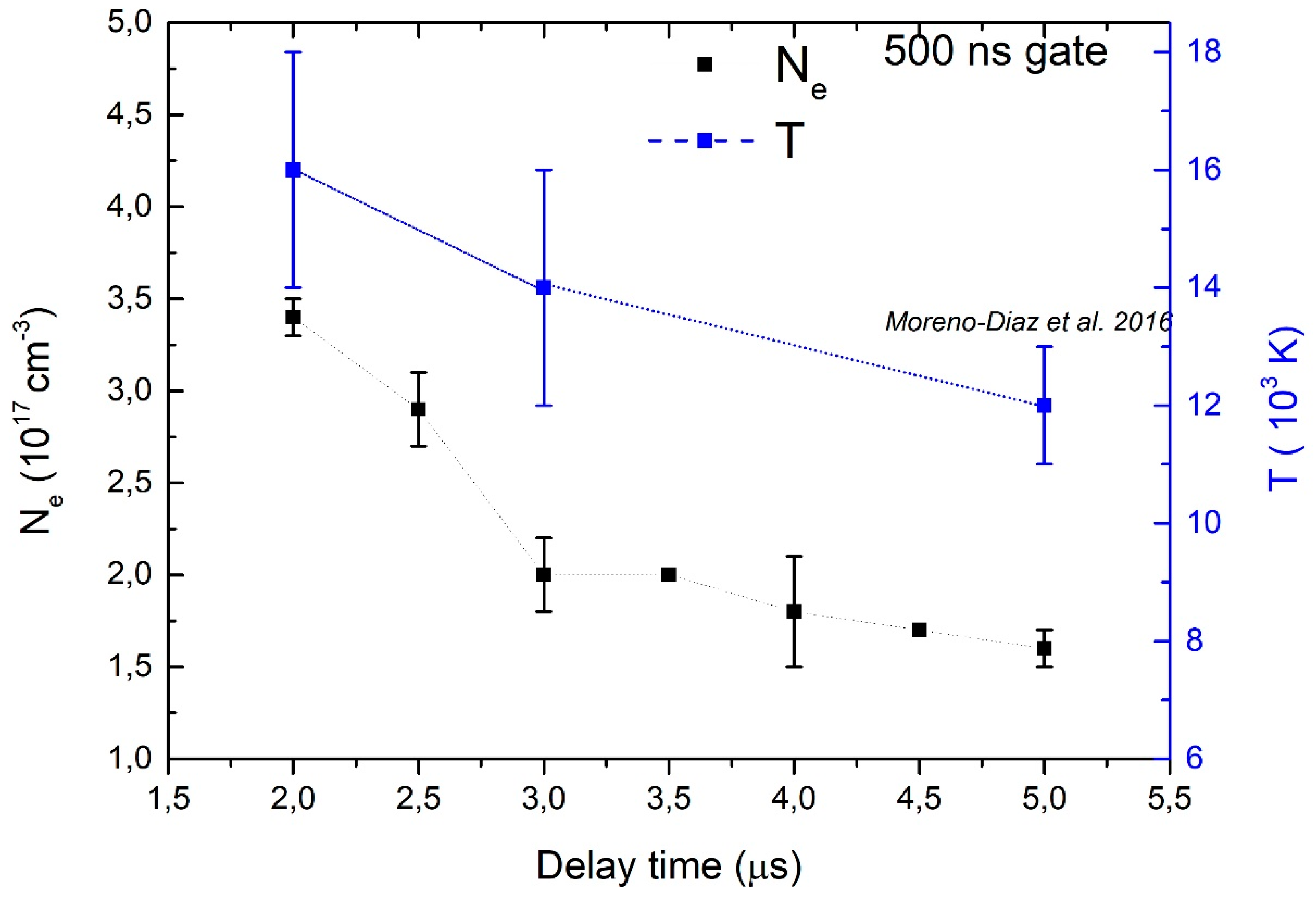
3.1.2. Electron Temperatures

As in the previous work (Moreno-Diaz et al. [24]), the electron temperature can be estimated by a Boltzmann plot under the assumption that the plasma is in local thermodynamic equilibrium (LTE) (Griem [27]; Griem [29]) using:
Iijλ = (Aijgi/U(T))N·exp(−Ei/kT)
ln (Iijλ/Aijgi) = ln(N/U(T)) − (Ei/kT)
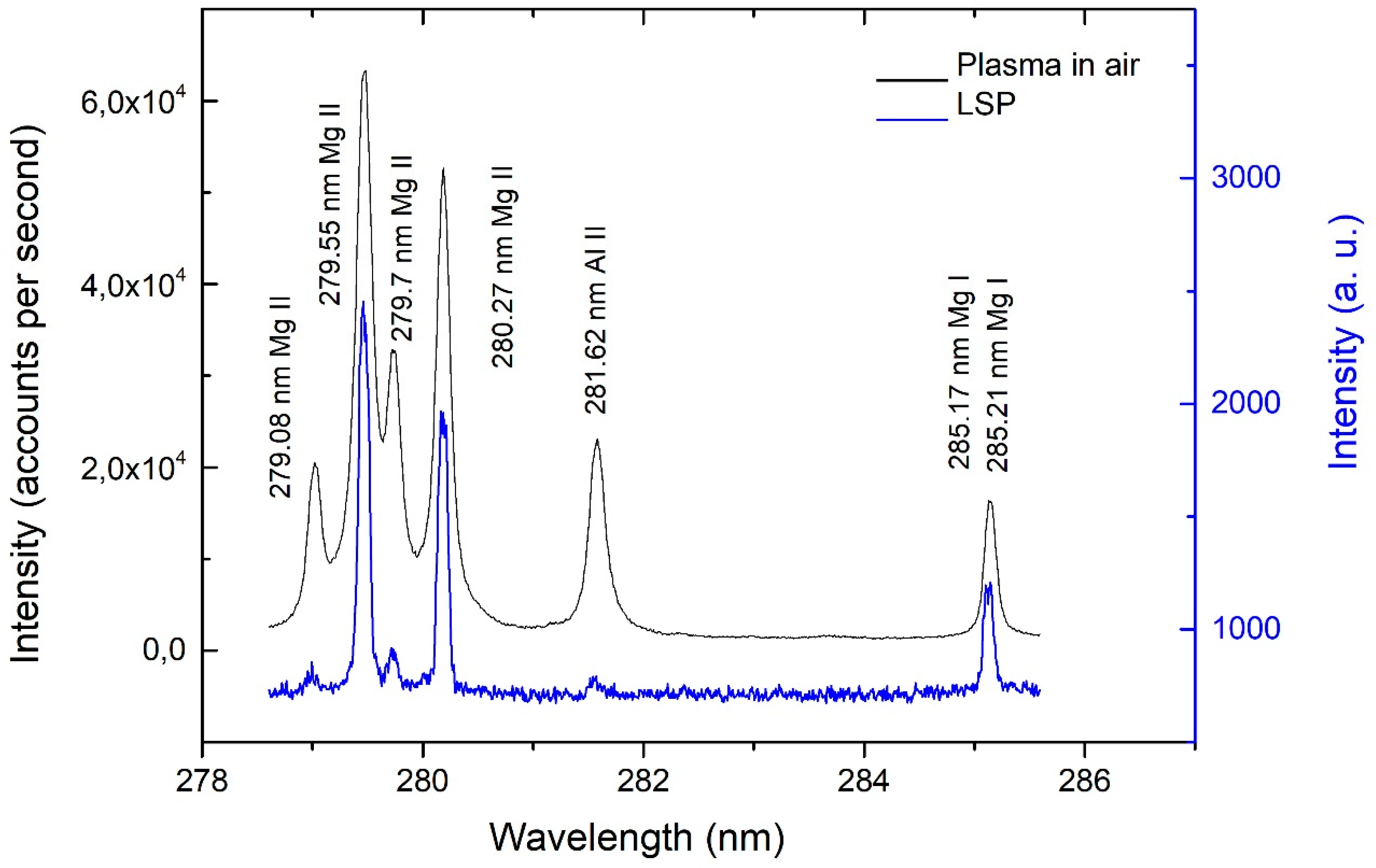
For a transition from a higher state i to a lower state j, I i j λ is the integrated measured integral line intensity in counts per second, Aij is the transition probability, λ is the wavelength of the transition, Ei is the excited level energy, gi is the energy and statistical weight of level i, U(T) is the atomic species partition function, N is the total density of emitting atoms, k is the Boltzmann constant, and T is the temperature in Kelvin. If the dependency of ln( I i j λ /Aijgi ) vs. Ei is plotted for lines of known transition probability (Boltzmann plot) the resulting straight line would have a slope of −1/kT, and, therefore, the temperature can be obtained without any previous knowledge of the total density of atoms or the atomic species partition function.
In several of the described cases, the temperature can be determined directly through this procedure because, as already mentioned, the emission of Mg II close to 279.5 nm, although weak, it was sufficient for the desired temperature estimation. Spectral lines used in the Boltzmann plot along with the transition probabilities and the energies corresponding to different starting levels were presented in Table 2 of the previous work (Moreno-Diaz et al. [24]). In addition, that table shows the ωref (impact broadening factors) measured by different authors that is necessary for the line self-absorption corrections.
In order to correct for the above mentioned self-absorption of Mg II lines, a procedure similar to that previously used and described in Moreno-Diaz et al. [24] was followed. Voigt profiles were adjusted to Mg II lines to determine their Lorentz broadening and apparent electron densities (Ne*). These values were then compared to the real electron densities (Ne), estimated from the Hα-line, in order to obtain the corresponding self-absorption (SA) coefficients in every line. Finally, with these coefficients, the relative intensity in the limit of null self-absorption (negligible self-absorption) was estimated.
An example of the results obtained by means of this procedure is displayed in Figure 7. In this Figure, for times up to 2 µs after laser pulse (500 ns temporal gate), a temperature of 18,700 ± 2000 K can be determined before correcting the line’s self-absorption. Once the self-absorption has been corrected, temperatures of 15,200 ± 2500 K are estimated. In the calculations, the uncertainty includes the statistical error from fitting of the temperature value and the statistical uncertainty in the intensities (~10%). These temperature values are maintained within the experimental range for temporal gates of 1000 ns and 2000 ns.
This process was also used for a 3 µs delay from the laser pulse and with those gate times where the intensity of the Mg II lines in the LSP conditions allowed for their discrimination from the background noise (500 ns and 1000 ns). The result obtained in this case was 14,000 ± 2500 K (using the self-absorption corrected values).
For delays equal to or greater than 3.5 ns, the estimation of the temperature by means of this method was been possible because of the lack of clear discrimination of the emission of the Mg II levels from the noise.
In a previous work of the authors (Moreno-Diaz et al. [24]) temperatures of about 10,900 K were estimated by means of an indirect procedure at a delay of 5 µs from the laser pulse. The values obtained here are in-line with that result and with the values that can be found in the bibliography without the presence of water (i.e., with ambient air).
The final results obtained in this work with this first procedure for electron densities and temperatures are shown in Figure 8. As it can be observed, the electron density and temperature decrease with an increase in the delay time. These values are similar to those obtained by other authors in similar experiments without water, as expected from the results obtained in previous work.

3.2. Second Method

In order to diagnose the plasma with a single experiment, the Stark width and the Stark shift of the Hα-line were used together for the first time in a combined way on the basis of the theoretical values of Griem [30] in the Equation (1). The experimental data presented in Table 1 were cross-checked with all the parameters provided by Griem and those situations that were coherent were conserved. As an example, for a 500 ns measurement window and a delay time of 4 µs, the experimental value obtained from Δλ1/2 = 14.4 ± 2.5 Å (see Figure 5), only provides a coherent value of electron density for the parameter α1/2 at the electron density of (1.78 ± 0.3) × 1017 cm−3 and at the temperature of 14,000 ± 2000 K. With a parameter α1/2 corresponding to any other pair of values of electron density and temperature, the numerical results obtained would not be consistent. If Ne = 1017 cm−3 and T = 10,000 K are chosen, the tabulated value of α1/2 would be 0.0186, which would give an electron density of 1.729 × 1017 cm−3 (about 70% different to the initial value of 1017 cm−3).
By using this method, the values for Ne and T presented in Table 3 were obtained. To confirm these results, the red shift values of the measured Hα-line were compared to the theoretical values provided by different authors [20,29] for the electron densities and the temperatures estimated in this work. An example of this comparison is presented in Table 4. In most cases the obtained value was very close to the theoretical values of these authors within the acknowledged experimental uncertainty levels, which allows us to state that the estimated values for electron density and temperature were consistent with the experimental results for the widths and shifts obtained in this work.

4. Discussion

According to the obtained results, both presented methods provide about the same values of electronic densities, but the second method leads to temperature values higher (around a 1.7 factor) than those obtained by the first procedure, as can be seen in Table 5. In this table, values of 5, 3, and 2 µs for the delay times and 500 ns for the time gate (with the best time of integration of the light) were used.
The authors consider that this deviation (that must not be considered as dramatic provided the general uncertainties considered in the kind of plasma diagnosis envisaged in the paper) may be attributed to the inherent inaccuracy of the procedure used to estimate the Hα-line shifts. Finer adjustments of the profile of the line (beyond a Voigt profile and considering asymmetries) are expected to yield more precise values of the temperatures using the described combinations of Stark widths and Stark shifts as described in the second method. In view of the promising character of this method for a practical determination of plasma parameters in one single step, these kinds of improvements are under way and are the subject of upcoming research.
The most important feature of the presented development and its comparison to the standard procedures is that within the experimental uncertainties, the authors consider that the described second method is sufficiently precise and practical to be implemented at an industrial level of LSP applications.
In view of the results obtained with the 500 ns window, we think that this second method based on both the Stark broadening and Stark shift of the Hα-line allows for the diagnosis of the plasma in industrial conditions, with good precision for the electron density and an acceptable uncertainty for temperature

5. Conclusions

In the present paper, the problem of direct spectroscopic monitoring of the laser induced plasma in water confined LSP processes is discussed as a feasible procedure aimed at answering the existing need for the development of process monitoring and control in industrial-scope applications. The authors present a procedure of diagnosis in relevant LSP conditions (confining water flow) using the spectroscopic possibilities offered by the Stark broadening and shift of the Hα-line (656.27 nm) to estimate electron densities and temperatures. The procedure has been demonstrated for the case of Al2024-T351 alloy using the luminescence of Mg II lines emitted by the traces of this element present in the alloy.
A Q-switched laser of Nd:YAG (2.5 J per pulse, 10 ns of pulse duration) was focused on an aluminum sample (Al2024-T351) used as the demonstrator. The Stark width and shift of the Balmer Hα-line (656.27 nm) was obtained with different delay times after the pulse of the laser (2–5 µs) and with several gate times (100, 200, 300, 500, and 1000 ns). The electron densities and electronic temperatures were estimated from this experimental data, the procedure being reproducible for any alloy containing Mg traces without lack of generality.
The measurement of the electronic temperature was performed directly under realistic LSP conditions. In the relevant experiments, the electron density and the temperature ranged between 1.2 × 10¹⁷ and 3.5 × 1017 cm−3 and between 10,000 and 16,000 K, respectively. These values are similar to those obtained by other authors in similar experiments without water. The best time of integration of the light was found to be about 500 ns. The rest of measured windows present different types of problems due to a lack of statistics or because they exceed the plasma evolution times (in the case of the 1000 ns gate time), this parameter being adjustable for each particular case of interest.
The novelty of the presented work stems from its proved capability to estimate the mentioned parameters under realistic water-confined LSP conditions using an improved procedure over previous developments, allowing single, direct determinations and shorter delay times from the laser pulse incidence. This procedure to estimate both electronic density and temperature density by a single experimental determination is considered an improvement on the existing plasma monitoring of LSP processes and opens the door for the much needed real-time monitoring of plasma behavior.

Author Contributions

Conceptualization: C.C., A.A.-M., J.L.O., M.I.d.A.-G.; Methodology: C.C., A.A.-M., J.L.O., J.A.P., M.I.d.A.-G., C.M.-D.; Investigation: C.C., A.A.-M., J.L.O., J.A.P., M.I.d.A.-G., C.M.-D., I.A.; Writing—review and editing: C.C., M.I.d.A.-G.

Funding

This work was financially supported by the Spanish DGI project MAT2015- 63974-C4-2-R.

Conflicts of Interest

The authors declare no conflict of interest.

References

  1. Askar’yan, G.A.; Moroz, E.M. Pressure on evaporation of matter in a radiation beam. JETP 1963, 16, 1638–1644. [Google Scholar]
  2. Fairand, B.P.; Wilcox, B.A.; Gallagher, W.J.; Willians, D.N. Laser Shock-Induced microstructural and mechanical property changes in 7075 Aluminum. J. Appl. Phys. 1972, 43, 3893–3895. [Google Scholar] [CrossRef]
  3. Yang, L.C. Stress waves generated in thin metallic films by a Q-switched ruby laser. J. Appl. Phys. 1974, 45, 2601–2607. [Google Scholar] [CrossRef]
  4. Fabbro, R.; Foumier, J.; Ballard, P.; Devaux, D.; Virmont, J. Physical study of laser-produced plasma in confined geometry. J. Appl. Phys. 1990, 68, 775–784. [Google Scholar] [CrossRef]
  5. Berthe, L.; Fabbro, R.; Peyre, P.; Tollier, L.; Bartnicki, E. Shock waves from a water-confined laser-generated plasma. J. Appl. Phys. 1997, 82, 2826–2833. [Google Scholar] [CrossRef]
  6. Sano, Y.; Mukai, N.; Okazaki, K.; Obata, M. Residual stress improvement in metal surface by underwater laser irradiation. Nucl. Instrum. Methods Phys. Res. B 1997, 121, 432–436. [Google Scholar] [CrossRef]
  7. Morales, M.; Porro, J.A.; Blasco, M.; Molpeceres, C.; Ocaña, J.L. Numerical simulation of plasma dynamics in laser shock processing experiments. Appl. Surf. Sci. 2009, 255, 5181–5185. [Google Scholar] [CrossRef]
  8. Ocaña, J.L.; Molpeceres, C.; Porro, J.A.; Gómez, G.; Morales, M. Experimental assessment of the influence of irradiation parameters on surface deformation and residual stresses in laser shock processed metallic alloys. Appl. Surf. Sci. 2004, 238, 501–505. [Google Scholar] [CrossRef]
  9. Martí-López, L.; Ocaña, R.; Porro, J.A.; Morales, M.; Ocaña, J.L. Optical observation of shock waves and cavitation bubbles in high intensity laser-induced shock processes. Appl. Opt. 2009, 48, 3671–3680. [Google Scholar] [CrossRef]
  10. Ocaña, J.L.; Correa, C.; Porro, J.A.; Díaz, M.; Ruiz de Lara, L.; Peral, D. Induction of through-thickness compressive residual stress fields in thin Al2024-T351 plates by laser shock processing. IJMSI 2015, 6, 725–736. [Google Scholar] [CrossRef] [Green Version]
  11. Correa, C.; Peral, D.; Porro, J.A.; Díaz, M.; Ruiz de Lara, L.; García-Beltrán, A.; Ocaña, J.L. Random-type scanning patterns in laser shock peening without absorbing coating in 2024-T351 Al alloy: A solution to reduce residual stress anisotropy. Opt. Laser Technol. 2015, 73, 179–187. [Google Scholar] [CrossRef]
  12. Wu, B.; Shin, C. A self-closed thermal model for laser shock peening under the water confinement regime configuration and comparisons to experiments. J. Appl. Phys. 2005, 97, 113517-1–113517-11. [Google Scholar] [CrossRef]
  13. Morales, M.; Ocaña, J.L.; Molpeceres, C.; Porro, J.A.; García-Beltrán, A. Model based optimization criteria for the generation of deep compressive residual stress fields in high elastic limit metallic alloys by ns-laser shock processing. Surf. Coat. Technol. 2008, 202, 2257–2262. [Google Scholar] [CrossRef] [Green Version]
  14. Ocaña, J.L.; Porro, J.A.; Morales, M.; Iordachescu, D.; Díaz, M.; Ruiz de Lara, L.; Correa, C.; Gil Santos, A. Laser Shock Processing: An emerging technique for the enhancement of surface properties and fatigue life of high-strength metal alloys. IJMMP 2013, 8, 38–52. [Google Scholar] [CrossRef]
  15. Musazzi, S.; Perini, U. Laser Induced Breakdown Spectroscopy Theory and Applications; Springer: Berlin, Germany, 2014. [Google Scholar]
  16. Colón, C.; Alonso-Medina, A. Application of a laser produced plasma. Experimental Stark widths of single ionized lead lines. Spectrochim. Acta B 2006, 61, 856–863. [Google Scholar] [CrossRef]
  17. Alonso-Medina, A. Measured Stark widths of several spectral lines of Pb III. Spectrochim. Acta B 2011, 66, 439–443. [Google Scholar] [CrossRef] [Green Version]
  18. Noll, R.; Sturm, V.; Aydin, Ü.; Eilers, D.; Gehlen, C.; Höhne, M.; Lamott, A.; Makowe, J.; Vrenegor, J. Laser-induced breakdown spectroscopy—From research to industry, new frontiers for process control. Spectrochim. Acta B 2008, 63, 1159–1166. [Google Scholar] [CrossRef]
  19. El Sherbini, A.M.; Heagzy, H.; El Sherbini, T.M. Measurement of electron density utilizing the Hα-line from laser produced plasma in air. Spectrochim. Acta B 2006, 61, 532–539. [Google Scholar] [CrossRef]
  20. Parigger, C.G.; Oks, E. Hydrogen Balmer series spectroscopy in laser-induced breakdown plasmas International. IRAMP 2010, 1, 13–23. [Google Scholar]
  21. El Sherbini, A.M.; Al Amer, A.A.S.; Hassan, A.T.; El Sherbini, T.M. Measurements of plasma electron temperature utilizing magnesium lines appeared in laser produced aluminum plasma in air. OPJ 2012, 2, 278–285. [Google Scholar] [CrossRef]
  22. De Giacomo, A.; Dell´aglio, M.; De Pascale, O. Single Pulse-Laser Induced Breakdown Spectroscopy in aqueous solution. Appl. Phys. A 2004, 79, 1035–1038. [Google Scholar] [CrossRef]
  23. Nath, A.; Khare, A. Spectroscopic Investigations on Laser Induced Breakdown in Water. J. Phys. Conf. Ser. 2010, 208, 012090-1–012090-4. [Google Scholar] [CrossRef]
  24. Moreno-Díaz, C.; Alonso-Medina, A.; Colón, C.; Porro, J.A.; Ocaña, J.L. Measurement of plasma electron density generated in an experiment of Laser Shock Processing, utilizing the Hα-line. J. Mater. Process. Technol. 2016, 232, 9–18. [Google Scholar] [CrossRef]
  25. Ocaña, J.L.; Molpeceres, C.; Morales, M.; Porro, J.A. Application of plasma monitoring methods to the optimized design of laser shock processing applications, High-Power Laser Ablation VI. Proc. SPIE 2006, 6261, 626124. [Google Scholar]
  26. Takata, T.; Enok, M.; Chivavibul, P.; Matsui, A.; Kobayashi, Y. Acoustic Emission Monitoring of Laser Shock Peening by Detection of Underwater Acoustic Wave. Mater. Trans. 2016, 57, 674–680. [Google Scholar] [CrossRef] [Green Version]
  27. Griem, H.R. Shift of hydrogen lines from electron collisions in dense plasmas. Phys. Rev. A 1983, 28, 1596–1601. [Google Scholar] [CrossRef]
  28. Ashkenazy, J.; Kipper, R.; Carner, M. Spectroscopic measurements of electron density of capillary plasma based on Stark broadening of hydrogen lines. Phys. Rev. A 1991, 43, 5568–5574. [Google Scholar] [CrossRef]
  29. Griem, H.R. Spectral Line Broadening by Plasmas; Elsvier: New York, NY, USA, 1974. [Google Scholar]
  30. Kepple, P.; Griem, H.R. Improved Stark profile calculations for the hydrogen lines Hα, Hβ, Hγ and Hδ. Phys. Rev. 1968, 173, 317–325. [Google Scholar] [CrossRef]
Figure 1. Experimental setup used in the reported Laser Shock Processing (LSP) experiments: (a) Scheme; (b) Photo.
Metals 09 00808 g001
Figure 2. A typical surface change after an LSP experiment. Images obtained via scanning confocal microscopy.
Metals 09 00808 g002
Figure 3. Mg II emission lines in air and LSP conditions. Delay time: 2 µs. Gate time: 1000 ns.
Metals 09 00808 g003
Figure 4. Spectrally resolved images of the plasma (with a gate time of 300 ns) at (a) 2.5 μs, (b) 4 μs, and (c) 5 μs after laser pulse with a wavelength range from 6530 to 6590 Å and spectra obtained from these images of the Hα-line in LSP conditions.
Metals 09 00808 g004
Figure 5. Fitting from a Voigt profile to experimental line emissions of the plasma with gate times of (a) 100 ns, (b) 300 ns, (c) 500 ns, and (d) 1000 ns at 4 µs delay time with a wavelength range from 6530 to 6590 Å.
Metals 09 00808 g005
Figure 6. Voigt profile fitting to experimental Hα-line emission of the plasma with a gate time of 500 ns at 4 µs delay time with a wavelength range from 6530 to 6590 Å.
Metals 09 00808 g006
Figure 7. Boltzmann plot for Mg II spectral lines from Laser Induced Plasma (Al 2024 target) in LSP conditions. The spectrum was recorded at a 2 µs delay time from the laser pulse and a gate time of 500 ns.
Metals 09 00808 g007
Figure 8. Electron density and electronic temperature versus delay time obtained with a gate time of 500 ns.
Metals 09 00808 g008
Table 1. Experimental Stark broadening (Δλ1/2 (Å)) and red Stark shift (d (Å)) of the Hα-line obtained in the LSP experiments of this work.
Time Delay (µs)1000 ns Gate500 ns Gate300 ns Gate200 ns Gate100 ns Gate
Δλ1/2 (Å)d (Å)Δλ1/2 (Å)d (Å)Δλ1/2 (Å)d (Å)Δλ1/2 (Å)d (Å)Δλ1/2 (Å)d (Å)
5.0 13.0 ± 0.51.013.8 ± 0.41.013.3 ± 0.41.011.5 ± 0.9(1.1)11.8 ± 3.1(1.0)
4.5 13.0 ± 1.41.113.9 ± 0.11.014.5 ± 0.20.912.3 ± 2.7(1.0)13.9 ± 0.2(1.0)
4.0 13.4 ± 2.91.214.4 ± 2.51.214.5 ± 2.21.114.7 ± 1.9(1.2)15.3 ± 0.7(1.1)
3.5 14.6 ± 0.11.215.6 ± 2.41.415.9 ± 1.81.516.8 ± 1.9(1.6)17.1 ± 3.9(1.7)
3.0 17.2 ± 0.61.515.7 ± 1.91.317.2 ± 0.81.917.7 ± 0.8(2.0)16.9 ± 1.9(1.7)
2.5 17.5 ± 2.51.820.2 ± 1.42.219.4 ± 3.42.419.6 ± 3.0(2.5)20.4 ± 5.3(2.3)
2.0 18.7 ± 2.02.122.5 ± 0.42.622.5 ± 7.42.818.7 ± 2.3(3.0)21.0 ± 4.5(-)
Table 2. Electron densities deduced from experimental values of Stark broadening of the Hα-line obtained in the LSP experiments of this work.
Time Delay
(µs)
1000 ns Gate500 ns Gate300 ns Gate200 ns Gate100 ns Gate
Ne
(1017 cm−3)
Ne
(1017 cm−3)
Ne
(1017 cm−3)
Ne
(1017 cm−3)
Ne
(1017 cm−3)
5.0 1.5 ± 0.11.6 ± 0.11.5 ± 0.11.2 ± 0.11.3 ± 0.3
4.5 1.5 ± 0.21.7 ± 0.11.8 ± 0.11.4 ± 0.31.7 ± 0.1
4.0 1.6 ± 0.41.8 ± 0.31.8 ± 0.31.8 ± 0.22.0 ± 0.1
3.5 1.8 ± 0.12.0 ± 0.32.1 ± 0.22.1 ± 0.32.4 ± 0.6
3.0 2.3 ± 0.12.0 ± 0.22.4 ± 0.12.4 ± 0.12.4 ± 0.3
2.5 2.3 ± 0.32.9 ± 0.22.8 ± 0.12.8 ± 0.43.1 ± 0.8
2.0 2.6 ± 0.33.4 ± 0.13.5 ± 1.12.7 ± 0.33.2 ± 0.7
Table 3. Electron densities and temperatures deduced from experimental values of Stark broadening of the Hα-line obtained in the LSP experiments of this work. Ne is 1017 cm−3 units and T is 103 K units.
Delay (µs)1000 ns Gate500 ns Gate300 ns Gate200 ns Gate100 ns Gate
NeTNeTNeTNeTNeT
5.0 1.5 ± 0.1131.6 ± 0.1131.5 ± 0.1101.2 ± 0.1101.3 ± 0.313
4.5 1.5 ± 0.2131.7 ± 0.1131.8 ± 0.1171.4 ± 0.3141.7 ± 0.118
4.0 1.6 ± 0.4141.8 ± 0.3141.8 ± 0.3211.8 ± 0.2152.0 ± 0.122
3.5 1.8 ± 0.1162.0 ± 0.3152.1 ± 0.2232.1 ± 0.3182.4 ± 0.627
3.0 2.3 ± 0.1182.0 ± 0.2192.4 ± 0.1242.4 ± 0.1202.4 ± 0.328
2.5 2.4 ± 0.3202.9 ± 0.2212.8 ± 0.1252.8 ± 0.4233.1 ± 0.828
2.0 2.7 ± 0.3263.4 ± 0.1243.5 ± 1.1272.7 ± 0.3273.2 ± 0.728
Table 4. Experimental Stark shifts of the Hα-line obtained in this work compared to the theoretical values found in the literature.
Delay (µs)1000 ns Gate500 ns Gate300 ns Gate
d (Å) This Workd (Å) Griemd (Å) Oksd (Å) This Workd (Å) Griemd (Å) Oksd (Å) This Workd (Å) Griemd (Å) Oks
5.01.00.90.61.00.90.61.00.90.6
4.51.10.90.61.01.00.70.91.20.8
4.01.21.00.71.21.10.71.11.30.9
3.51.21.20.81.41.30.81.51.51.0
3.01.51.61.11.31.40.91.91.81.3
2.51.81.71.22.22.11.42.42.21.5
2.02.12.21.52.62.61.82.82.81.9
Table 5. Electronic temperatures obtained from Boltzmann plot compared with the temperatures estimated from red shifts of the Hα-line obtained in this work at 5, 3, and 2 µs delay times and 500 ns of time gate.
Ne (1017 cm−3)T (103 K) from Boltzmann plotd (Å) Griem a)d (Å) This WorkT (103 K) from Red Shifts
1.6 ± 0.1110.81.013
2.0 ± 0.2141.11.318
3.4 ± 0.1151.82.626
a) Griem [30].

