Corrosion Behaviour of L80 Steel Grade in Geothermal Power Plants in Switzerland


Abstract
:1. Introduction
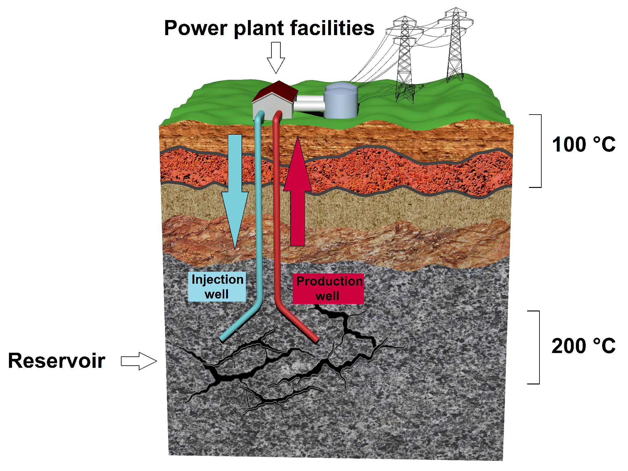
1.1. Corrosion in Binary Geothermal Power Plants
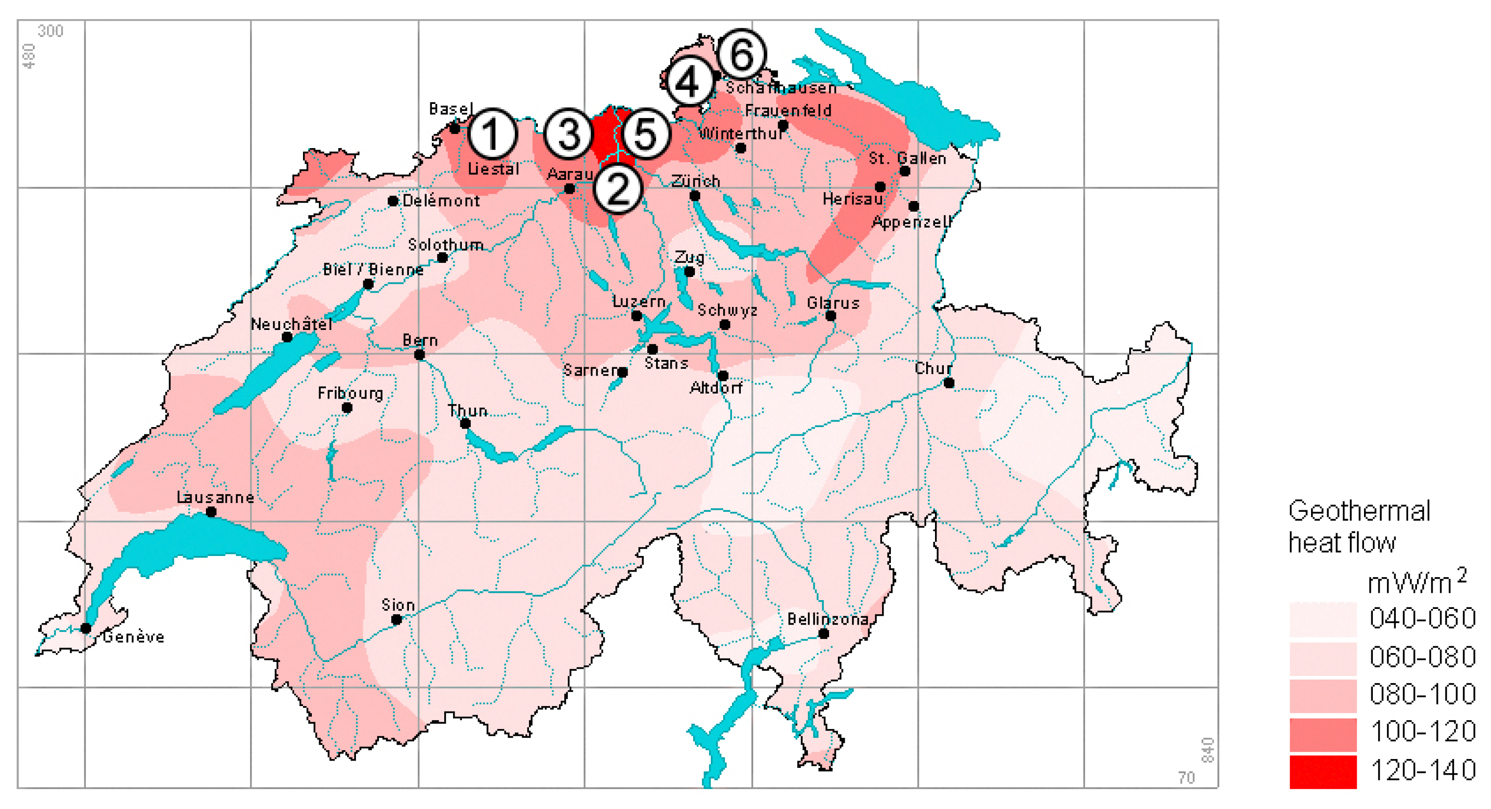
1.2. Representative Swiss Geothermal Fluids
2. Materials and Methods
2.1. Synthetic Geothermal Fluids
2.2. Materials
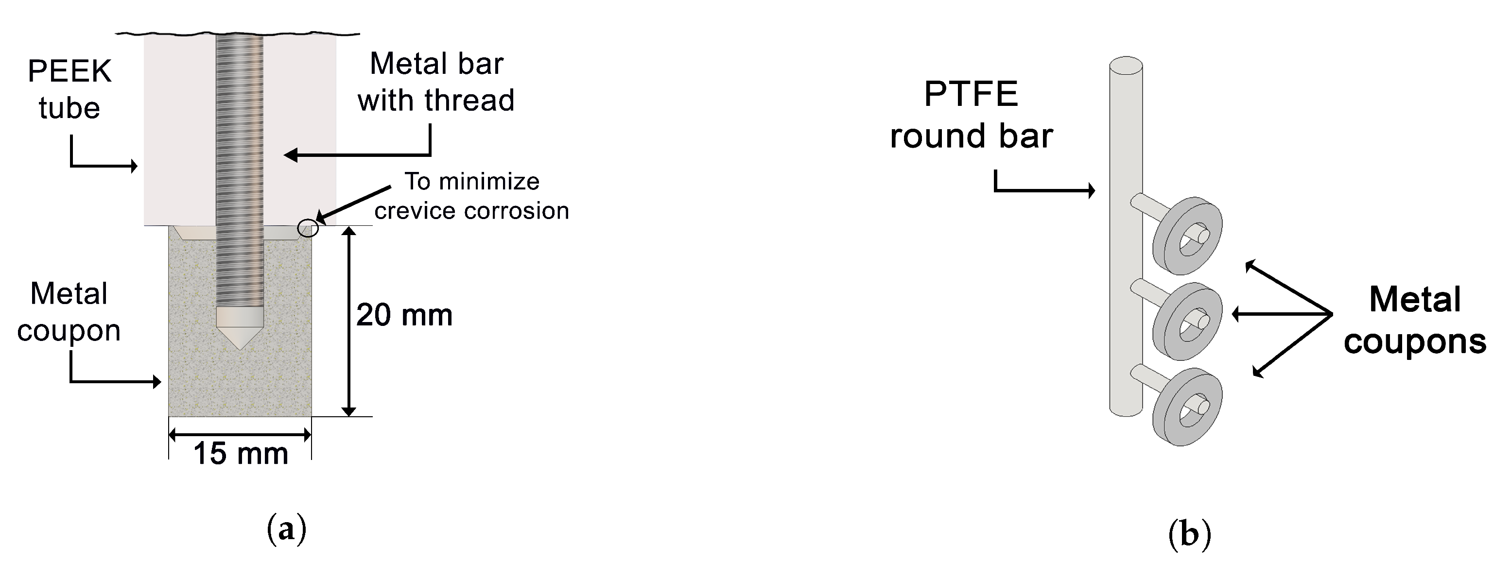
2.3. Experimental Procedures
2.3.1. Electrochemical Measurements at High Temperature and Pressure
2.3.2. Gravimetric Experiments
2.3.3. Analysis Post-Exposure
3. Results
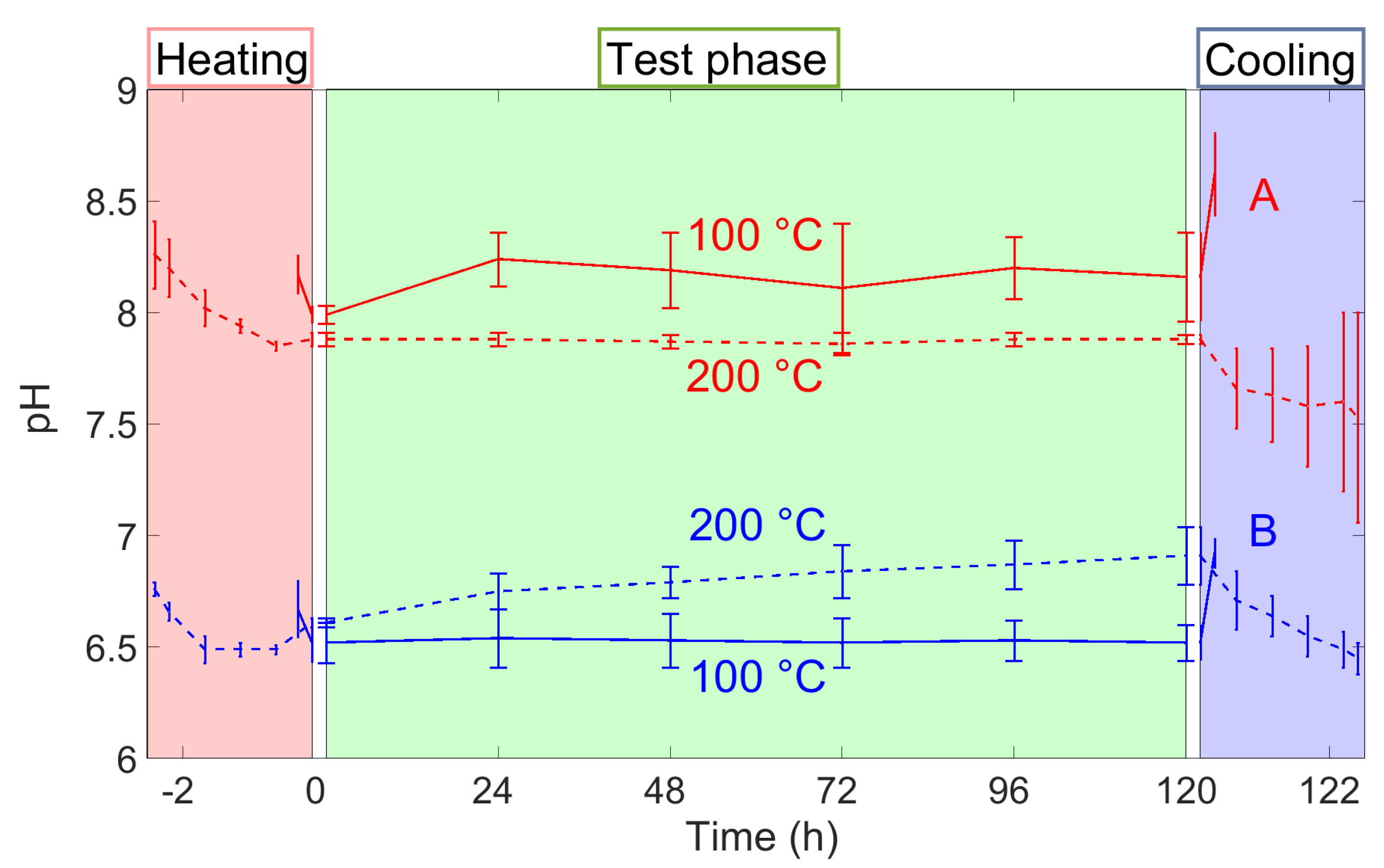
3.1. pH Evolution
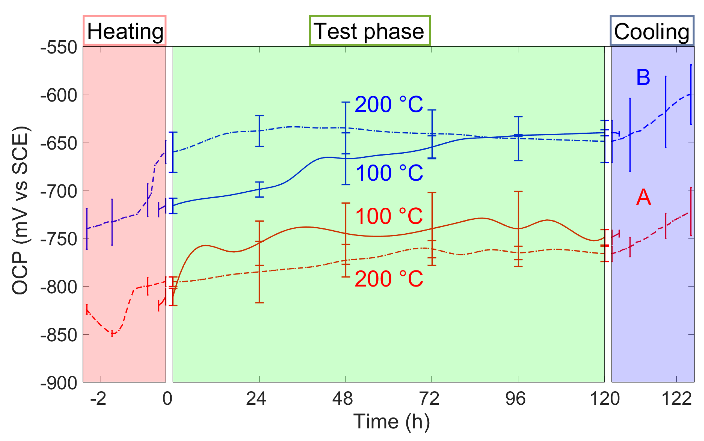
3.2. Open Circuit Potential (OCP) Evolution
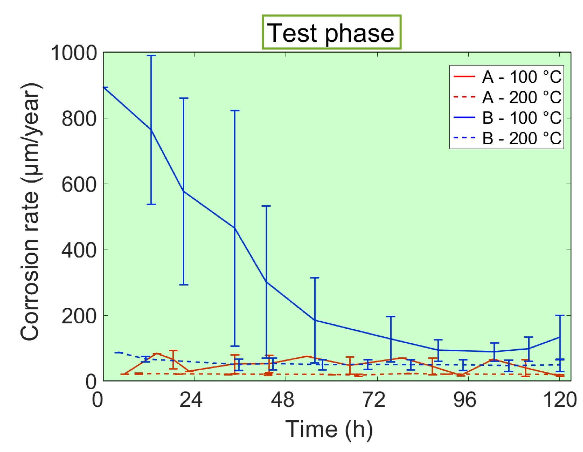
3.3. Corrosion Rates
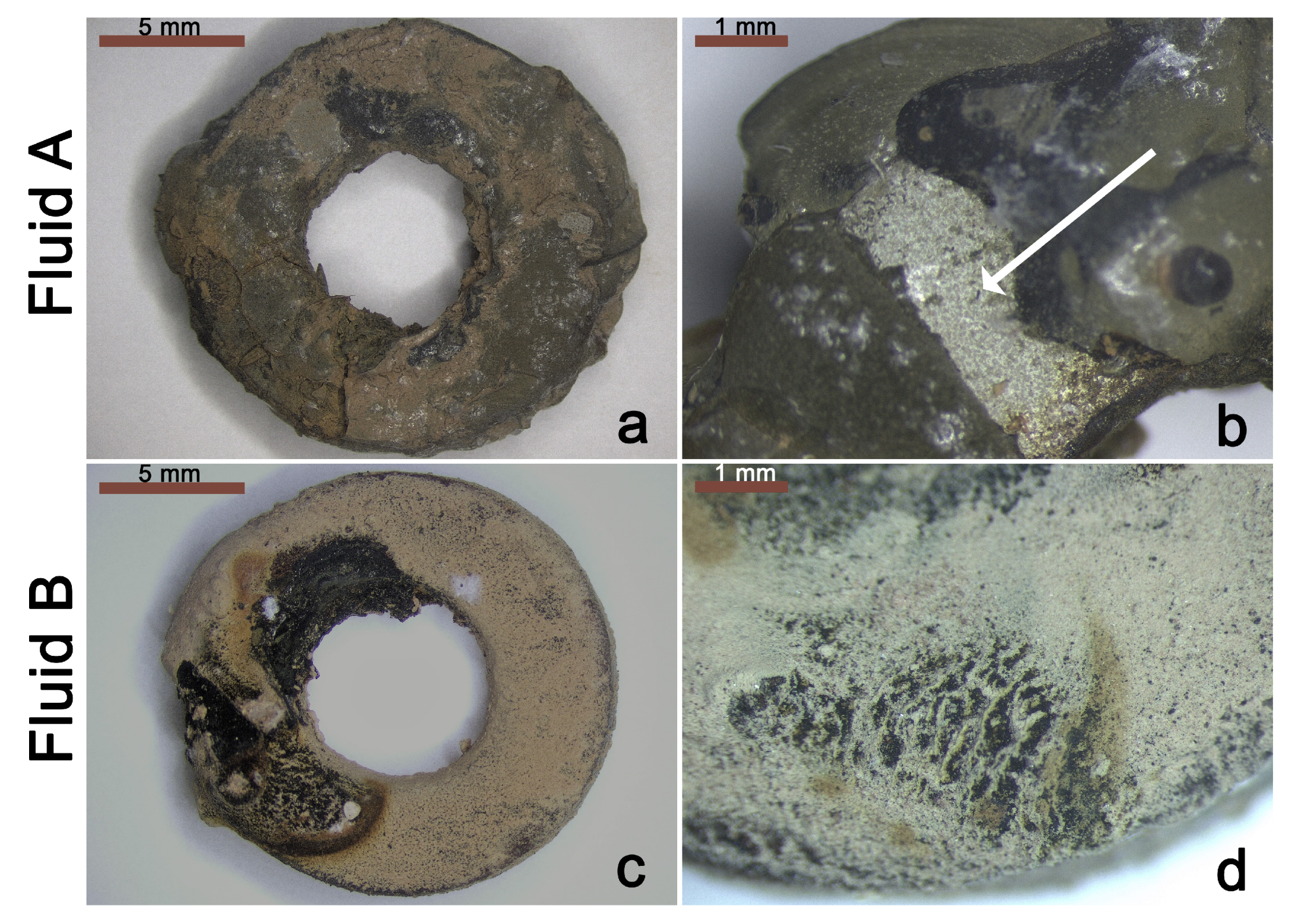
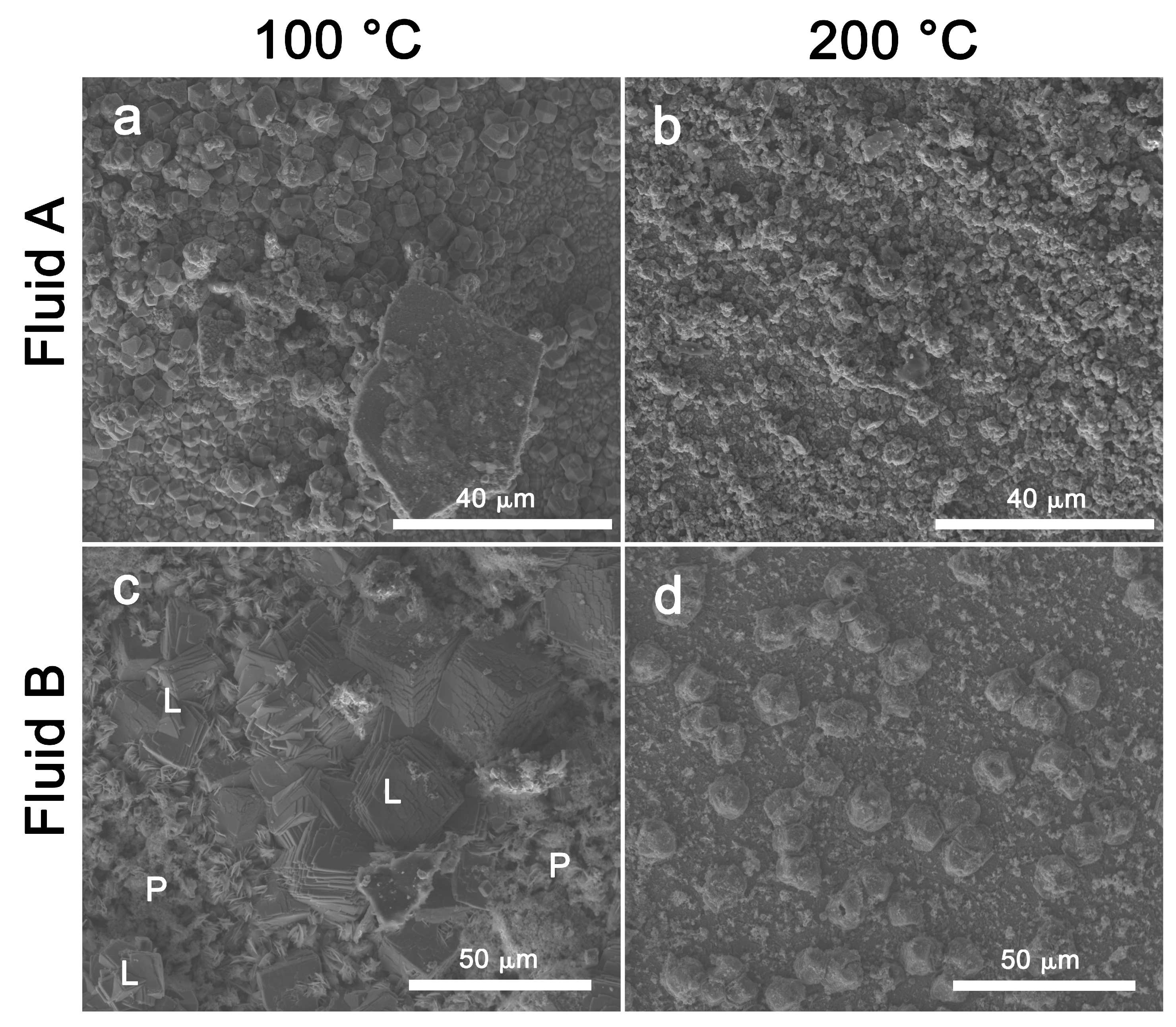
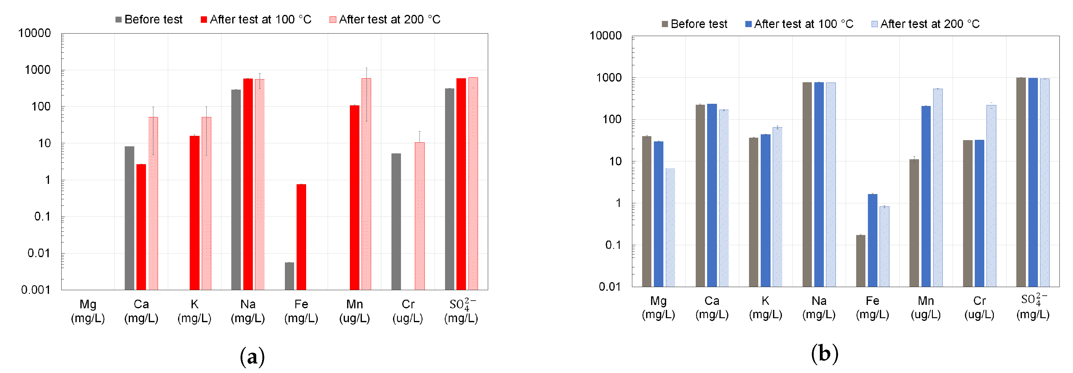
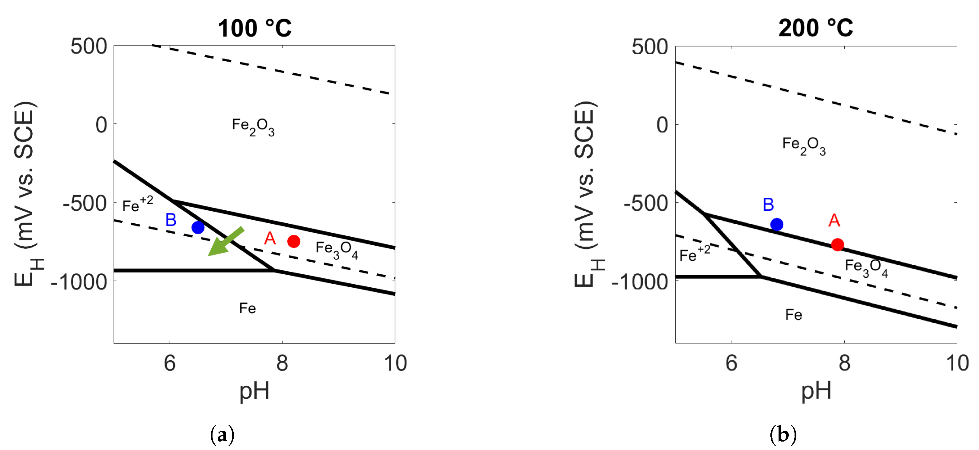
3.4. Surface and Fluid Analyses
4. Discussion
5. Conclusions
Supplementary Materials
Author Contributions
Funding
Acknowledgments
Conflicts of Interest
References
- Dickson, M.H.; Fanelli, M. Geothermal Energy: Utilization and Technology, 1st ed.; Routledge: London, UK, 2013; ISBN 978-18-4407-184-5. [Google Scholar]
- Barbier, E. Geothermal energy technology and current status: An overview. Renew. Sustain. Energy Rev. 2002, 6, 3–65. [Google Scholar] [CrossRef]
- Li, K.; Bian, H.; Liu, C.; Zhang, D.; Yang, Y. Comparison of geothermal with solar and wind power generation systems. Renew. Sustain. Energy Rev. 2015, 42, 1464–1474. [Google Scholar] [CrossRef]
- Ellabban, O.; Abu-Rub, H.; Blaabjerg, F. Renewable energy resources: Current status, future prospects and their enabling technology. Renew. Sustain. Energy Rev. 2014, 39, 748–764. [Google Scholar] [CrossRef]
- Fridleifsson, I.B.; Bertani, R.; Huenges, E.; Lund, J.W.; Ragnarsson, A.; Rybach, L. The possible role and contribution of geothermal energy to the mitigation of climate change. In Proceedings of the IPCC Scoping Meeting on Renewable Energy Sources, Luebeck, Germany, 20–25 January 2008; pp. 59–80. [Google Scholar]
- Fridleifsson, I.B. Geothermal energy for the benefit of the people. Renew. Sustain. Energy Rev. 2001, 5, 299–312. [Google Scholar] [CrossRef] [Green Version]
- Swiss Federal Office of Energy. Energy Strategy 2050 once the New Energy Act is in Force. Available online: http://www.bfe.admin.ch/energiestrategie2050/ (accessed on 3 January 2019).
- Hirschberg, S.; Wiemer, S.; Burgherr, P. (Eds.) Energy from the Earth: Deep Geothermal as a Resource for the Future? vdf Hochschulverlag AG: Zurich, Switzerland, 2015; ISBN 978-3-7281-3654-1. [Google Scholar]
- Olasolo, P.; Juárez, M.C.; Morales, M.P.; Liarte, I.A. Enhanced geothermal systems (EGS): A review. Renew. Sustain. Energy Rev. 2016, 56, 133–144. [Google Scholar] [CrossRef]
- Wyss, R.; Link, K. Actual Developments in Deep Geothermal Energy in Switzerland. In Proceedings of the World Geothermal Congress 2015, Melbourne, Australia, 19–25 April 2015. [Google Scholar]
- Link, K.; Rybach, L.; Imhasly, S.; Wyss, R. Geothermal Energy in Switzerland—Country Update. In Proceedings of the World Geothermal Congress 2015, Melbourne, Australia, 19–25 April 2015. [Google Scholar]
- Genter, A.; Guillou-Frottier, L.; Feybesse, J.L.; Nicol, N.; Dezayes, C.; Schwartz, S. Typology of potential hot fractured rock resources in Europe. Geothermics 2003, 32, 701–710. [Google Scholar] [CrossRef]
- Huenges, E. (Ed.) Geothermal Energy Systems: Exploration, Development, and Utilization; John Wiley and Sons: New York, NY, USA, 2010; ISBN 978-3-527-64461-2. [Google Scholar]
- Tester, J.W.; Anderson, B.J.; Batchelor, A.S.; Blackwell, D.D.; DiPippo, R.; Drake, E.M.; Garnish, J.; Livesay, B.; Moore, M.C.; Nichols, K.; et al. The Future of Geothermal Energy: Impact of Enhanced Geothermal Systems (EGS) on the United States in the 21st Century; Massachusetts Institute of Technology: Cambridge, MA, USA, 2006; Volume 209. [Google Scholar]
- Finger, J.; Blankenship, D. Handbook of Best Practices for Geothermal Drilling; Sandia National Laboratories: Albuquerque, NM, USA, 2010. [Google Scholar]
- DiPippo, R. Geothermal Power Plants: Principles, Applications, Case Studies and Environmental Impact, 4th ed.; Butterworth-Heinemann: Oxford, UK, 2015; ISBN 978-00-8100-879-9. [Google Scholar]
- Majer, E.L.; Baria, R.; Stark, M.; Oates, S.; Bommer, J.; Smith, B.; Asanuma, H. Induced seismicity associated with enhanced geothermal systems. Geothermics 2007, 36, 185–222. [Google Scholar] [CrossRef]
- Evans, K.F.; Zappone, A.; Kraft, T.; Deichmann, N.; Moia, F. A survey of the induced seismic responses to fluid injection in geothermal and CO2 reservoirs in Europe. Geothermics 2012, 41, 30–54. [Google Scholar] [CrossRef]
- Zang, A.; Oye, V.; Jousset, P.; Deichmann, N.; Gritto, R.; McGarr, A.; Majer, E.; Bruhn, D. Analysis of induced seismicity in geothermal reservoirs—An overview. Geothermics 2014, 52, 6–21. [Google Scholar] [CrossRef]
- Mundhenk, N.; Huttenloch, P.; Sanjuan, B.; Kohl, T.; Steger, H.; Zorn, R. Corrosion and scaling as interrelated phenomena in an operating geothermal power plant. Corros. Sci. 2013, 70, 17–28. [Google Scholar] [CrossRef]
- Karlsdóttir, S.N. Corrosion, scaling and material selection in geothermal power production. In Comprehensive Renewable Energy; Sayigh, A., Ed.; Elsevier: Amsterdam, The Netherlands, 2012; Volume 7, pp. 241–259. ISBN 978-0-08-087873-7. [Google Scholar]
- Goldberg, A.; Owen, L.B. Pitting corrosion and scaling of carbon steels in geothermal brine. Corrosion 1979, 35, 114–124. [Google Scholar] [CrossRef]
- Schreiber, S.; Lapanje, A.; Ramsak, P.; Breembroek, G. (Eds.) Operational Issues in Geothermal Energy in Europe: Status and Overview; Geothermal ERA NET: Reykjavik, Iceland, 2016; ISBN 978-9979-68-397-1. [Google Scholar]
- Ellis, P.F.; Conover, M.F. Materials Selection Guidelines for Geothermal Energy Utilization Systems; Radian Corp.: Austin, TX, USA, 1981. [Google Scholar]
- Iberl, P.; Alt, N.S.A.; Schluecker, E. Evaluation of corrosion of materials for application in geothermal systems in Central Europe. Mater. Corros. 2015, 66, 733–755. [Google Scholar] [CrossRef]
- Frick, S.; Regenspurg, S.; Kranz, S.; Milsch, H.; Saadat, A.; Francke, H.; Brandt, W.; Huenges, E. Geochemical and process engineering challenges for geothermal power generation. Chem. Ing. Tech. 2011, 83, 2093–2104. [Google Scholar] [CrossRef]
- Bertani, R. Geothermal power generation in the world 2010–2014 update report. Geothermics 2016, 60, 31–43. [Google Scholar] [CrossRef]
- Regenspurg, S.; Wiersberg, T.; Brandt, W.; Huenges, E.; Saadat, A.; Schmidt, K.; Zimmermann, G. Geochemical properties of saline geothermal fluids from the in-situ geothermal laboratory Groß Schönebeck (Germany). Chem. Erde-Geochem. 2010, 70, 3–12. [Google Scholar] [CrossRef]
- Mundhenk, N.; Huttenloch, P.; Kohl, T.; Steger, H.; Zorn, R. Metal corrosion in geothermal brine environments of the Upper Rhine graben – Laboratory and on-site studies. Geothermics 2013, 46, 14–21. [Google Scholar] [CrossRef]
- Miranda-Herrera, C.; Sauceda, I.; González-Sánchez, J.; Acuña, N. Corrosion degradation of pipeline carbon steels subjected to geothermal plant conditions. Anti-Corros. Methods Mater. 2010, 57, 167–172. [Google Scholar] [CrossRef]
- Karlsdóttir, S.N.; Hjaltason, S.M.; Ragnarsdottir, K.R. Corrosion behavior of materials in hydrogen sulfide abatement system at Hellisheiði geothermal power plant. Geothermics 2017, 70, 222–229. [Google Scholar] [CrossRef]
- Klapper, H.S.; Bäßler, R.; Sobetzki, J.; Weidauer, K.; Stürzbecher, D. Corrosion resistance of different steel grades in the geothermal fluid of Molasse Basin. Mater. Corros. 2013, 64, 764–771. [Google Scholar] [CrossRef]
- Czernichowski-Lauriol, I.; Fouillac, C. The chemistry of geothermal waters: its effects on exploitation. Terra Nova 1991, 3, 477–491. [Google Scholar] [CrossRef]
- Nicholson, K. Geothermal Fluids: Chemistry and Exploration Techniques; Springer: Berlin/Heidelberg, Germany, 1993; ISBN 978-3-642-77846-9. [Google Scholar]
- Breede, K.; Dzebisashvili, K.; Falcone, G. Overcoming challenges in the classification of deep geothermal potential. Geother. Energy Sci. 2015, 3, 19–39. [Google Scholar] [CrossRef] [Green Version]
- André, L.; Rabemanana, V.; Vuataz, F.D. Influence of water–rock interactions on fracture permeability of the deep reservoir at Soultz-sous-Forêts, France. Geothermics 2006, 35, 507–531. [Google Scholar] [CrossRef]
- Franco, A.; Villani, M. Optimal design of binary cycle power plants for water-dominated, medium-temperature geothermal fields. Geothermics 2009, 38, 379–391. [Google Scholar] [CrossRef] [Green Version]
- Genter, A.; Evans, K.; Cuenot, N.; Fritsch, D.; Sanjuan, B. Contribution of the exploration of deep crystalline fractured reservoir of Soultz to the knowledge of enhanced geothermal systems (EGS). C. R. Geosci. 2010, 342, 502–516. [Google Scholar] [CrossRef]
- Nogara, J.; Zarrouk, S.J. Corrosion in geothermal environment Part 2: Metals and alloys. Renew. Sustain. Energy Rev. 2018, 82, 1347–1363. [Google Scholar] [CrossRef]
- Feili, H.R.; Akar, N.; Lotfizadeh, H.; Bairampour, M.; Nasiri, S. Risk analysis of geothermal power plants using Failure Modes and Effects Analysis (FMEA) technique. Energy Convers. Manag. 2013, 72, 69–76. [Google Scholar] [CrossRef]
- Nogara, J.; Zarrouk, S.J. Corrosion in geothermal environment: Part 1: Fluids and their impact. Renew. Sustain. Energy Rev. 2018, 82, 1333–1346. [Google Scholar] [CrossRef]
- Sonney, R.; Vuataz, F.D. Properties of geothermal fluids in Switzerland: A new interactive database. Geothermics 2008, 37, 496–509. [Google Scholar] [CrossRef] [Green Version]
- Bodmer, P.; Rybach, L. Heat flow maps and deep ground water circulation: Examples from Switzerland. J. Geodyn. 1985, 4, 233–245. [Google Scholar] [CrossRef]
- Breede, K.; Dzebisashvili, K.; Liu, X.; Falcone, G. A systematic review of enhanced (or engineered) geothermal systems: Past, present and future. Geother. Energy 2013, 1, 4. [Google Scholar] [CrossRef]
- Medici, F.; Rybach, L. Geothermal Map of Switzerland 1995 (Heat Flow Density); Commission Suisse de Géophysique: Zurich, Switzerland, 1995; No. 30. [Google Scholar]
- CREGE (Centre de Recherche en Geothermie). BDFGeotherm—Web Database of Geothermal Fluids in Switzerland. Available online: https://crege.ch/index.php?menu=down&page=rd_BDFGeothem (accessed on 15 March 2016).
- API Specification 5CT. Specification for Casing and Tubing, 8th ed.; API Publishing Services: Washington, DC, USA, 2005. [Google Scholar]
- Vallejo Vitaller, A.; Angst, U.M.; Elsener, B. Setup of an electrochemical test cell for studying corrosion of steels for geothermal applications. Manuscript in preparation.
- Stern, M.; Geary, A.L. Electrochemical polarization I. A theoretical analysis of the shape of polarization curves. J. Electrochem. Soc. 1957, 104, 56–63. [Google Scholar] [CrossRef]
- Bard, A.J.; Faulkner, L.R. Electrochemical Methods: Fundamentals and Applications, 2nd ed.; John Wiley and Sons: New York, NY, USA, 2001; ISBN 978-0-471-04372-0. [Google Scholar]
- Jones, D.A. Principles and Prevention of Corrosion, 2nd ed.; Prentice-Hall: Upper Saddle River, NJ, USA, 1996; pp. 143–167. ISBN 0-13-359993-0. [Google Scholar]
- ASTM G31-12a. Standard Guide for Laboratory Immersion Corrosion Testing of Metals; ASTM International: West Conshohocken, PA, USA, 2012. [Google Scholar]
- ASTM G 1-03. Standard Practice for Preparing, Cleaning, and Evaluating Corrosion Test Specimens; ASTM International: West Conshohocken, PA, USA, 2011. [Google Scholar]
- Beverskog, B.; Puigdomenech, I. Revised Pourbaix diagrams for iron at 25–300 ∘C. Corros. Sci. 1996, 38, 2121–2135. [Google Scholar] [CrossRef]
- Linnenbom, V.J. The Reaction between Iron and Water in the Absence of Oxygen. J. Electrochem. Soc. 1958, 105, 322–324. [Google Scholar] [CrossRef]
- Tagirov, B.R.; Diakonov, I.I.; Devina, O.A.; Zotov, A.V. Standard ferric–ferrous potential and stability of FeCl to 90 ∘C. Thermodynamic properties of Fe (aq) 3+ and ferric-chloride species. Chem. Geol. 2000, 162, 193–219. [Google Scholar] [CrossRef]
- Shannon, D.W. Corrosion of Iron-Base Alloys Versus Alternate Materials in Geothermal Brines; (Interim Report No. PNL-2456); Pacific Northwest Laboratories: Richland, WA, USA, 1977.


| Fluid | pH | Temp () | Ca2+ | Mg2+ | Na+ | K+ | HCO– | SO2– | Cl– |
|---|---|---|---|---|---|---|---|---|---|
| 1 | 6.50 | 25.8 | 260.0 | 45.6 | 856.0 | 35.0 | 1423.0 | 950.0 | 556.0 |
| 2 | 6.78 | 30.7 | 88.0 | 21.0 | 2712.0 | 168.0 | 891.0 | 793.0 | 3555.0 |
| 3 | 7.93 | 34.9 | 34.1 | 3.0 | 363.5 | 24.2 | 366.0 | 532.0 | 73.1 |
| 4 | 8.2 | 57 | 5.5 | 0.4 | 172.1 | 4.6 | 281.0 | 64.0 | 27.0 |
| 5 | 8.25 | 31.3 | 8.5 | 0.2 | 395.4 | 8.3 | 372.0 | 339.0 | 142.0 |
| 6 | 8.8 | 47 | 6.0 | 0.7 | 172.1 | 3.8 | 267.0 | 71.0 | 25.0 |
| Fluid | pH | Ca2+ | Mg2+ | Na+ | K+ | HCO– | SO2– | Cl– |
|---|---|---|---|---|---|---|---|---|
| A | 8.4–9.0 | 10.0 | - | 282.8 | - | 399.8 | 300.0 | - |
| B | 6.5–7.4 | 250.0 | 45.0 | 747.0 | 35.0 | 1400.0 | 900.0 | 600.0 |
| Steel Sample | wt.% (and Fe bal.) | ||||||||||
|---|---|---|---|---|---|---|---|---|---|---|---|
| Composition | C | Si | Mn | Cr | Mo | S | P | Ni | Cu | Al | V |
| L80 Type 1 | 0.25 | 0.19 | 1.02 | 0.45 | 0.16 | 0.004 | 0.014 | 0.04 | 0.02 | 0.03 | 0.003 |
| Temperature | Fluid | Corrosion Rate (μm/year) | |
|---|---|---|---|
| Gravimetric Tests (720 h) | Electrochemical Tests (120 h) | ||
| 100 | A | 92 ± 22 | 48 ± 11 |
| B | 245 ± 43 | 308 ± 136 | |
| 200 | A | - | 19 ± 1 |
| B | - | 52 ± 14 | |
© 2019 by the authors. Licensee MDPI, Basel, Switzerland. This article is an open access article distributed under the terms and conditions of the Creative Commons Attribution (CC BY) license (http://creativecommons.org/licenses/by/4.0/).
Share and Cite
Vallejo Vitaller, A.; Angst, U.M.; Elsener, B. Corrosion Behaviour of L80 Steel Grade in Geothermal Power Plants in Switzerland. Metals 2019, 9, 331. https://doi.org/10.3390/met9030331
Vallejo Vitaller A, Angst UM, Elsener B. Corrosion Behaviour of L80 Steel Grade in Geothermal Power Plants in Switzerland. Metals. 2019; 9(3):331. https://doi.org/10.3390/met9030331
Chicago/Turabian StyleVallejo Vitaller, Ana, Ueli M. Angst, and Bernhard Elsener. 2019. "Corrosion Behaviour of L80 Steel Grade in Geothermal Power Plants in Switzerland" Metals 9, no. 3: 331. https://doi.org/10.3390/met9030331