Article

Quantifying the Contribution of Crystallographic Texture and Grain Morphology on the Elastic and Plastic Anisotropy of bcc Steel

1
Max-Planck-Institut für Eisenforschung GmbH, Max-Planck-Straße 1, 40237 Düsseldorf, Germany
2
Division of Physical Metallurgy, Materials Science Department, TU Darmstadt, Alarich-Weiss-Straße 2, 64287 Darmstadt, Germany
*
Author to whom correspondence should be addressed.
Current address: Department of Materials Science and Engineering, University of California Los Angeles, Los Angeles, CA 90095, USA.
Metals 2019, 9(12), 1252; https://doi.org/10.3390/met9121252
Submission received: 24 September 2019 / Revised: 24 October 2019 / Accepted: 25 October 2019 / Published: 22 November 2019
(This article belongs to the Special Issue Dislocation Mechanics of Metal Plasticity and Fracturing)

Abstract

:
The influence of grain shape and crystallographic orientation on the global and local elastic and plastic behaviour of strongly textured materials is investigated with the help of full-field simulations based on texture data from electron backscatter diffraction (EBSD) measurements. To this end, eight different microstructures are generated from experimental data of a high-strength low-alloy (HSLA) steel processed by linear flow splitting. It is shown that the most significant factor on the global elastic stress–strain response (i.e., Young’s modulus) is the crystallographic texture. Therefore, simple texture-based models and an analytic expression based on the geometric mean to determine the orientation dependent Young’s modulus are able to give accurate predictions. In contrast, with regards to the plastic anisotropy (i.e., yield stress), simple analytic approaches based on the calculation of the Taylor factor, yield different results than full-field microstructure simulations. Moreover, in the case of full-field models, the selected microstructure representation influences the outcome of the simulations. In addition, the full-field simulations, allow to investigate the micro-mechanical fields, which are not readily available from the analytic expressions. As the stress–strain partitioning visible from these fields is the underlying reason for the observed macroscopic behaviour, studying them makes it possible to evaluate the microstructure representations with respect to their capabilities of reproducing experimental results.

1. Introduction

The plastic deformation induced during processing of metallic materials typically results in strong crystallographic textures and, thereby, macroscopically anisotropic mechanical properties. The prime example for such a process is the cold rolling of metal sheets, which is used for processing such diverse materials as aluminum, magnesium and steel. As the anisotropic elastic and plastic behaviour induced by texture and grain morphology has a significant influence on formability and dimensional accuracy, it is imperative to account for the anisotropy when conducting high-precision metal forming simulations [1]. However, the direct multi-scale inclusion of all microstructure details is usually computationally prohibitive. Approaches to reduce the computational efforts include model order reduction schemes [2,3], the use of Statistically Similar Representative Volume Elements (SSRVEs) [4] and homogenization methods like the Relaxed Grain Cluster (RGC) scheme by Tjahjanto et al. [5]. Despite these efforts to include microstructure details, usually analytic yield surface descriptions are employed to include plastic anisotropy. The superior execution speed of analytic yield descriptions, though, comes often at the price of significant experimental efforts associated with calibrating their constitutive parameters. Especially for complex yield surface descriptions (Banabic [6] gives a detailed overview), which require to probe the materials response in multiple deformation modes, it is therefore desirable to (partly) replace experiments by micro-mechanical simulations using numerical methods such as the Finite Element Method (FEM) [7] or Fast Fourier Transform (FFT) based spectral methods [8]. Gawad et al. [9] extended this concept in their “Hierarchical Multi-Scale Model” (HMS) by performing on-the-fly yield surface computations.
All approaches that aim at improving the quality of component-scale simulations by taking the average material response from the homogenized polycrystal response are based on two ingredients: a description of grain morphology and texture as well as a suitable model for the single crystal behaviour. In this study, different approaches for microstructure and texture representation (i.e., the first ingredient) are compared with respect to their ability to correctly predict the elastic and plastic anisotropy of a strongly textured material. The materials constitutive behaviour (i.e., the second ingredient) is described with a crystal plasticity formulation that is classified as “phenomenological” by Roters et al. [10].
It should be noted that CPFEM studies with similar aims have already been performed 20 to 30 years ago [11,12,13,14]. While most of these studies were focused on the investigation of texture development, the ability of the CPFEM approach to predict average mechanical properties was also shown. However, the increase in computational capacities allows now to redo such investigations with much higher spatial resolution. In this study, more than two million discrete points—each with its directly measured orientation—are used for each individual simulation while in the early days of CPFEM modeling even a few hundreds of thousands elements was associated with long computation times.
The material investigated here is a high-strength low-alloy (HSLA) steel processed by linear flow splitting. The linear flow splitting process, presented in detail by Groche et al. [15], is used to produce bifurcated profiles in an integral style. It enables the manufacturing of sheet metal products with improved quality at lower costs [16] in comparison to conventional, multistep production routes. From previous investigations by Bruder et al. [17] it is known that the microstructure of the produced profile has a crystallographic texture and grain morphology that resembles that of cold rolled body-centred cubic (bcc) steels [18]. With regards to further processing of parts produced by the novel linear flow splitting technique, an accurate description of the resulting anisotropic material properties and their implementation in metal forming simulations is of great importance for exploiting the full potential of this technique. In a previous study by Niehuesbernd et al. [19], the elastic anisotropy induced by linear flow splitting in the investigated HSLA steel has been characterized experimentally and compared to predictions from analytic models based on the measured crystallographic texture. It was shown that the effective orientation dependent Young’s modulus can be accurately predicted from the crystallographic information when the geometric mean is used to calculate the polycrystalline average from the the single crystal stiffness/compliance tensor. The values obtained from the geometric mean lie well in-between the upper bound resulting from the assumption of spatially constant strains introduced by Voigt [20] and the lower bound based on the assumption of spatially constant stress by Reuss [21]. In addition—and in contrast to other approaches such as the Hill [22] average—this averaging scheme gives the same results regardless whether the stiffness or the compliance tensor is used. However, the complete omission of the grain morphology might render this approach invalid for the elongated grains of the probed material (compare the work of Jöchen et al. [23]). The present study therefore aims at evaluating the impact of the grain aspect ratio on the elastic and plastic behaviour of strongly textured microstructures by means of full-field simulations. To this end, results from numerical simulations employing microstructure representations of different degrees of sophistication are compared to simple analytic, texture-based models.
The study is structured as follows—First, details of the investigated material, including production steps and employed characterization methods, are given. The following section deals with the used numerical simulation method and the employed approaches for constructing microstructure representations from experimental data. The results are presented in Section 4 and compared and discussed with respect to the performance of the various simulation approaches in Section 5. After that, the conclusions that can be drawn from the results and the associated discussion are presented. The study finishes with an outlook on how to improve the predictive quality of crystal plasticity simulations.

2. Material: Composition, Processing and Characterization

The investigated material is an H480LA HSLA steel with a carbon content of 0.07 wt . % ; details of the material are presented by Niehuesbernd et al. [19]. The microstructure of the material in as-received condition consists of ferrite grains and small cementite particles at the grain boundaries. Linear flow splitting was carried out continuously in 10 stages to produce double-Y-profiles with 12 m m long and 1 m m thick flanges (see Figure 1) from the initial sheet with a thickness of 2 m m .
Three mutually perpendicular cross sections parallel to normal direction (ND), rolling direction (RD) and transverse direction (TD) of the flanges were produced (see Figure 1) for texture and microstructure investigations. Sample preparation for Electron Backscatter Diffraction (EBSD) was performed using standard metallographic grinding and polishing techniques followed by an additional polishing step with an aqueous suspension of 0.05 μ m Al2O3 particles. Subsequent EBSD measurements were carried out on all three samples with a Tescan Mira3 feg scanning electron microscope at a distance of 170 μ m from the flange top surface. The size of the characterized area was adapted to the microstructure so that the maps contained at least 2000 grains and about 2.5 million measurement points to ensure an accurate representation of texture data and grain morphologies at the same time. The three obtained microstructure maps are shown in Figure 2 with color code assigned according to the inverse pole figure (IPF) in the respective sample surface normal direction. It can be seen that the material exhibits a microstructure with highly elongated, “pancake shaped” grains (see Figure 2) with average grain dimensions of 0.2 μ m in ND, 0.8 μ m in TD and 1.4 μ m in RD. The apparent grain aspect ratios in the cross sectional measurements are therefore about 6.9 in the RD-section, 4.0 in the TD-section and 1.7 in the ND-section. The microstructure features a strong bcc-rolling texture including a distinct α-fiber (〈110〉 ‖ RD) with a dominant rotated cube orientation ({001}〈110〉 (the {001} crystal planes are parallel to the sheet plane (ND) and the 〈110〉 crystallographic directions are parallel to the rolling direction (RD).) having maximum intensity of about 20 times random and a typical γ-fiber (〈111〉 ‖ ND). The φ 2 = 45 -section of the orientation distribution function (ODF) of the texture data from the TD-section is shown in Figure 3.
Tensile tests were performed on the flange material in order to obtain experimental data on the plastic behaviour. For this purpose, dogbone-shaped tensile samples along TD, RD and under 45 between these directions were prepared (see Figure 1). The samples were ground from the flange top surface by 90 μ m and afterwards from the lower surface to a final thickness of 130 μ m in order to perform the tests at approximately the same positions as the microstructure investigations.
Without using numerical simulations, the orientation dependent Young’s modulus was directly estimated from the measured texture by computing the geometric mean of the stiffness tensor as:
C geom = exp 1 N i = 1 N ln T i T C T i .
Here, N is the number of measurement points, C the stiffness tensor in crystal coordinates (cube orientation) and T are rotation matrices obtained from the EBSD measurements. The Young’s modulus in any given direction is then calculated from this tensor for each direction. As shown by Niehuesbernd et al. [19], values provided by this approach fall well into the range determined from ultrasonic measurements, which is therefore preferred over more involved approaches [22,24].
Given the success of this averaging approach when calculating the elastic response, it was also used to calculate the average Taylor [25] factor M for prediction of the average plastic behaviour. To this end, the individual Taylor factor M i for uniaxial tension in the considered loading direction was calculated assuming slip on 〈111〉{110} and 〈111〉{112} slip systems with equal critical shear stresses on all slip systems for all orientations. Then, the geometric mean of these N Taylor factors is calculated according to the following equation:
M geom = exp 1 N i = 1 N ln M i .
The proof stress at 0.05% plastic deformation, σ y , from the tensile test along TD was selected to determine the apparent critical resolved shear stress τ CRSS . With the Taylor factor from the combined texture data of all three EBSD measurements a value of τ CRSS = 268   M Pa was determined via τ CRSS = σ y / M . This calculation is, however, only a rather rough approximation since it is based on the assumption of a homogeneous deformation of all points, irrespective of their crystallographic orientation. Moreover, this approximation does not take into account that different types of slip systems can have different critical resolved shear stresses. Nevertheless, this approach enables to analytically estimate the yield strength distribution for comparison with values obtained by numerical simulations and tensile tests.

3. Simulation Setup

The simulation setup, consisting of a microstructure representation, a constitutive law and a numerical solver for solving mechanical equilibrium under given boundary conditions, is outlined in the following.

3.1. Microstructure Representation

To investigate the influence of grain morphology and crystallographic texture on the global and local stress–strain behaviour, different microstructure representations are created based on the EBSD measurements presented in Section 2. While the first series of representations (I) is based on the individual data per measurement, all three measurements are combined for the second series (II) to increase the statistical reliability.
The five microstructure representations of series I based on the the three individual measurements are the following:
I a 
Direct takeover 2D: These 2D full-field models are based on a direct takeover of the measured crystallographic orientation on each of the 1601 × 1600 = 2,561,600 points (see Figure 2).
I b 
Random orientation assignment 2D: By randomly shuffling the measured crystallographic orientations among the points, a second set of 1601 × 1600 resolved 2D microstructures has been created.
I c 
Random orientation assignment 3D: The random distribution of almost all (Less than 2% of the discrete crystallographic orientations had to be discarded when distributing them on an equi-gridded cube ( 136 3 < 1601 × 1600 < 137 3 ).) measured orientations on a 3D grid with 136 × 136 × 136 = 2,515,456 points gives a third set of microstructure variants.
The latter two microstructure variants lack any information on grain morphology but contain the full information of the crystallographic texture. This can be clearly seen in Figure 4a, where the 3D model (I c) based on the ND-section data is shown. When applied to a component scale simulation, this approach results in microstructure representations similar to the ones used in the “Texture-Component Crystal Plasticity FEM” (TCCP-FEM) introduced by Roters and Zhao [26] and Böhlke et al. [27].
The orientation information, that is, texture, for the fourth and fifth set of microstructure representation is created in the following way: First, a discrete ODF with a bin size of 5.0 is created from the BungeEuler angle representation of the crystallographic orientations without taking the sample symmetry into account. Second, using the HybridIa method developed by Eisenlohr and Roters [28], the 1000 orientations that best represent the whole ODF are selected (see Reference [29] for a different approach to reduce the orientation data.). A comparison of texture index and entropy using MTEX 4.5.0 by Bachmann et al. [30] between the full texture and the selected orientation reveals a good approximation, especially there is no significant sharpening or weakening of the texture when using the approximation by 1000 orientations. This reduced texture is used for the following two representations in the first series:
I d 
2DVoronoitessellation: A regular grid of 2024 × 2024 = 4,096,576 pixel is divided into 1000 grains with a periodic Voronoi tessellation. Each grain gets a homogeneous initial orientation assigned.
I e 
3DVoronoitessellation: Similarly, a 160 × 160 × 160 = 4,096,000 voxel grid is divided into 1000 equiaxed grains with a periodic Voronoi tessellation. The resulting microstructure for the RD-section is shown in Figure 4b.
Three more microstructure representations are generated from the combined texture information of all three measurements to increase the statistical reliability. The same approach to reduce the texture data to 1000 orientations as for microstructures I d and I e is employed:
II a 
3D microstructure without grain information: This TCCP-FEM model is conceptually a combination of variant I c (Random orientation assignment 3D) and I e (3D Voronoi tessellation): 1000 orientations are assigned to the points of a 10 × 10 × 10 grid.
II b 
3D microstructure with globular grains: The same geometric representation as for variant I e (3D Voronoi tessellation) is used but the 1000 orientations represent the texture of all three measurements. To investigate the influence of the grain shape separately from the influence of the strong crystallographic texture present in the probed material, a variant of this microstructure is created in which 1000 randomly sampled orientations are assigned to the grains.
II c 
3D microstructure with elongated grains: To generate elongated grains, a standard Voronoi tesselation of 1000 seed points is performed on a 160 × 160 × ( 160 · 8 ) grid from which only every eights plane along the last direction is used. The resulting grain structure with a grain aspect ratio of 8:8:1 (RD:TD:ND) and initial homogeneous orientation per grain is shown in Figure 4c. To investigate the influence of the grain shape separately from the influence of the strong crystallographic texture present in the probed material, a variant of this microstructure is created in which 1000 randomly sampled orientations are assigned to the grains.
Preliminary control simulations have shown that the artificially created microstructures (I b to I e and II a to II c) are representative, that is, the statistical and macroscopic results considered here do not differ significantly. This finding is in agreement with a similar study on Dual Phase (DP) steels by Diehl [31] where measured microstructures where systematically coarsened.

3.2. Constitutive Model for Crystal Plasticity

A viscoplastic phenomenological formulation for crystal plasticity, introduced in similar form by Hutchinson [32] and Peirce et al. [33], is used in combination with an elastic stiffness tensor with cubic symmetry to describe the behaviour of the bcc material. This crystal plasticity model is based on the assumption that plastic slip γ occurs on a slip system α when the resolved shear stress τ α exceeds a critical value ξ α . The critical shear stress on each of the 24 slip systems is assumed to evolve from an initial value, ξ 0 to a saturation value ξ due to slip on the 12 〈111〉{110} and 12 〈111〉{112} systems according to the relation ξ ˙ α = h 0 | γ ˙ β | | 1 ξ β / ξ β | a sgn ( 1 ξ β / ξ β ) h α β with initial hardening h 0 , interaction coefficients h α β , a numerical parameter a and β = 1 , , 24 . The shear rate on system α is then computed as γ ˙ α = γ ˙ 0 | τ α / ξ α | n sgn ( τ α / ξ α ) with the inverse shear rate sensitivity n and reference shear rate γ ˙ 0 . The sum of the shear rates on all systems determines the plastic velocity gradient L p in the employed finite strain formulation. Values for the single crystal stiffness tensor of iron at room temperature are known with good precision from experiments [34,35]. Here the values from the latter reference, given in Table 1a, are used. Parameters for the plastic behaviour (Table 1b) are based on parameters used by Tasan et al. [36], however, ξ 0 and ξ have been re-scaled by a constant factor such that model II c (3D microstructure with elongated grains) loaded in TD-direction reproduces the experimentally obtained proof stress. The constitutive formulation is implemented in the Düsseldorf Advanced Material Simulation Kit (DAMASK, presented in detail by Roters et al. [37,38]) where it can be used with different solvers for mechanical equilibrium, i.e., the commercial finite element solvers MSC.Marc and Abaqus and an efficient FFT-based spectral solver. The latter one is used in this study, details are given in the following.

3.3. Numerical Solver and Boundary Conditions

An FFT-based spectral solver is employed to solve for static mechanical equilibrium. It is based on the finite strain extension by Lahellec et al. [39] of the well-established formulation by Moulinec and Suquet [40], Lebensohn [41]; details regarding formulation, implementation and numerical performance are presented in References [42,43]. This solver operates on a regular grid, which allows the direct point-wise takeover of the EBSD data. Since an infinite medium is assumed, the data is periodically repeated in all three directions, which introduces artifacts at the boundary if the investigated microstructure is not periodic. For an infinite body, the applied boundary conditions are volume averages which in the employed large-strain formulation are given in mutually exclusive components of deformation gradient F and first PiolaKirchhoff stress P . Uniaxial loading along 16 different directions at a rate of 0.0002 s 1 was applied in 25 increments of 1 s duration, i.e., until a final technical strain of 0.5% was reached. In case of loading the ND-section (Figure 2a), loading varied from θ = 0.0 (along RD, horizontal) to θ = 168.75 in 11.25 steps, i.e., θ = 90.0 corresponds to loading along TD (vertical direction) and a rotation by θ = 180.0 is equivalent to no rotation ( θ = 0.0 ). The corresponding deformation gradient, first PiolaKirchhoff stress tensor and rotation matrix read as
F = 1.0 + x 0.0 0.0 0.0 0.0 0.0 0.0
P = 0.0 0.0
R = + cos ( θ ) sin ( θ ) 0.0 + sin ( θ ) + cos ( θ ) 0.0 0.0 0.0 1.0 .
Here, the symbol “*” indicates an undefined component since values in F and P are mutually exclusive. The strain x in the ( 11 ) component of F is set to 0.005 (0.5%) and θ measures the angle between RD and TD along ND.

4. Results

The simulation results are presented in the following. First, to quantify the average elastic and plastic behaviour, the orientation dependent Young’s modulus (E) and yield stress ( σ y ) are given and compared to the corresponding results from the analytic calculations (Section 4.1). Then the local stress–strain distribution of selected simulations is presented in Section 4.2 to investigate in detail the differences at the micro-scale caused by the very different model assumptions.

4.1. Average Behaviour

Young’s modulus E resulting from the simulations is calculated as E = σ / ε where σ is the average second PiolaKirchhoff stress and ε the average GreenLagrange strain along the loading direction at the first, purely elastic loading step.
Table 2 gives an overview of the obtained values for loading along ND, RD and TD. Table 2a shows that the simulation results obtained from the individual sections differ by at most + 4 G Pa and 3 G Pa from the analytic results and Table 2b reveals even slightly smaller differences when using the combined texture ( + 3 G Pa and 2 G Pa ). For both, analytic calculation and simulated results, the Young’s modulus along ND calculated from the RD-section is approximately 10 G Pa higher than the value obtained from the TD-section. The differences between these sections are, hence, significantly higher than among all full-field simulation approaches.
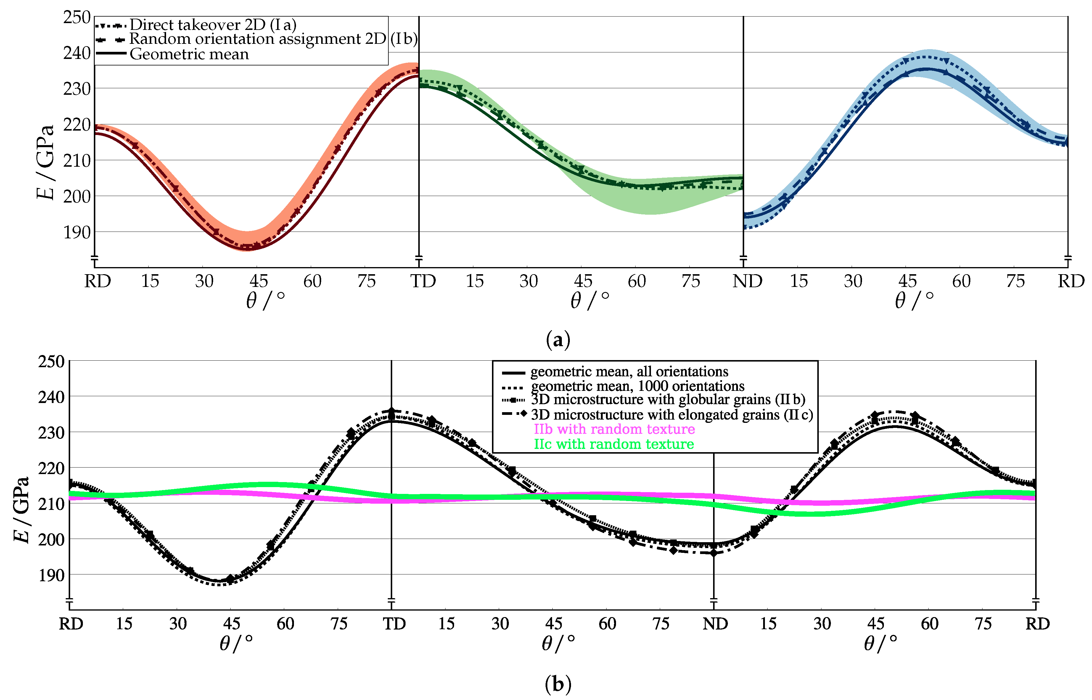
Figure 5 displays the course of Young’s modulus over the three mutually perpendicular sections corresponding to the measurements. As the symmetry of grain shape and crystallographic texture allows to average the values of loading directions with an angular difference of 90 around the sample normal, only values for half of the considered loading direction range (0 –180 ) are shown. A cubic spline interpolation was performed to obtain values between the rotation angles for which a simulation was conducted. The analytic calculation has been performed at steps of 1 , making an interpolation unnecessary. Figure 5a compares the results of the analytic calculation to both 2D simulations using the full set of orientations from the individual measurements (i.e., microstructure sets I a and I b). Additionally, the range observed among all five simulations (I a to I e) is given as a background color. Figure 5b shows results from the analytic and numerical calculations from the combination of the full texture information and the cases of a random texture (models II b and II c only).
Among all simulation results obtained from the individual measurements (Figure 5a) the relative difference computed as ( max ( a i ) min ( a i ) ) / avg ( a i ) is smaller than 2.0%, 3.0% and 4.0% for the RD-section, ND-section and the TD-section, respectively. Results obtained by the analytic calculation are very close to the simulation not taking the grain shape into account (microstructure variant I b). The largest deviations between the two simulation approaches in Figure 5a can be seen for loading along ND (RD-section at 90 , TD-section at 0 ), where the values obtained from the simulation including grain shape are lower by 4 G Pa and at 45 between ND and RD where the simulation including grain shape is higher by 4 G Pa . Overall, the influence of the grain morphology is rather small, a finding in agreement with a study by Jöchen et al. [23].
There are virtually no differences observable between the results from the analytic calculations using the complete orientation information obtained from all three measurements and its sample consisting of 1000 representative orientations, see Figure 5b. The same holds for the 3D models, where the use of globular (II b) and elongated (II c) grain shapes gives virtually the same results. Moreover, the differences between the simulations and the analytic calculations are smaller than 3 G Pa (less than 1.5%) for the whole orientation range (Figure 5b).
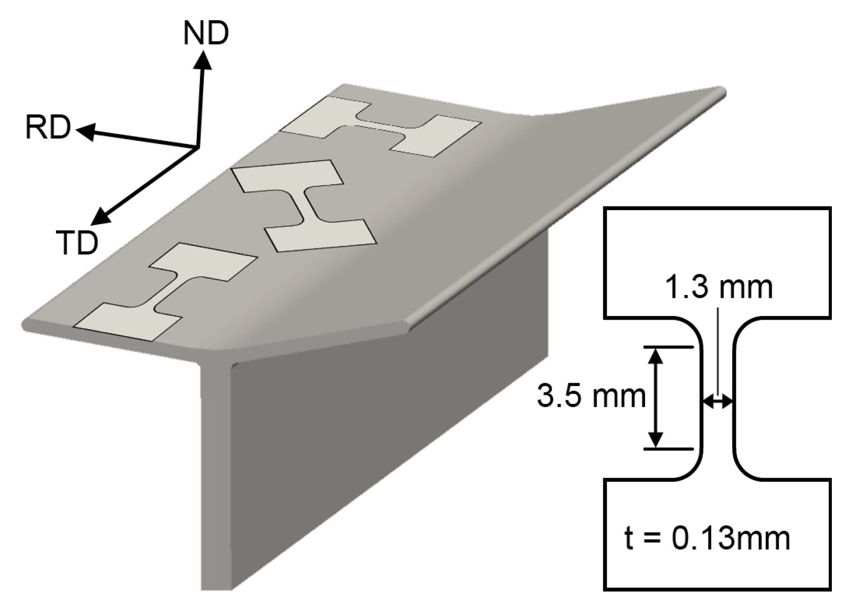
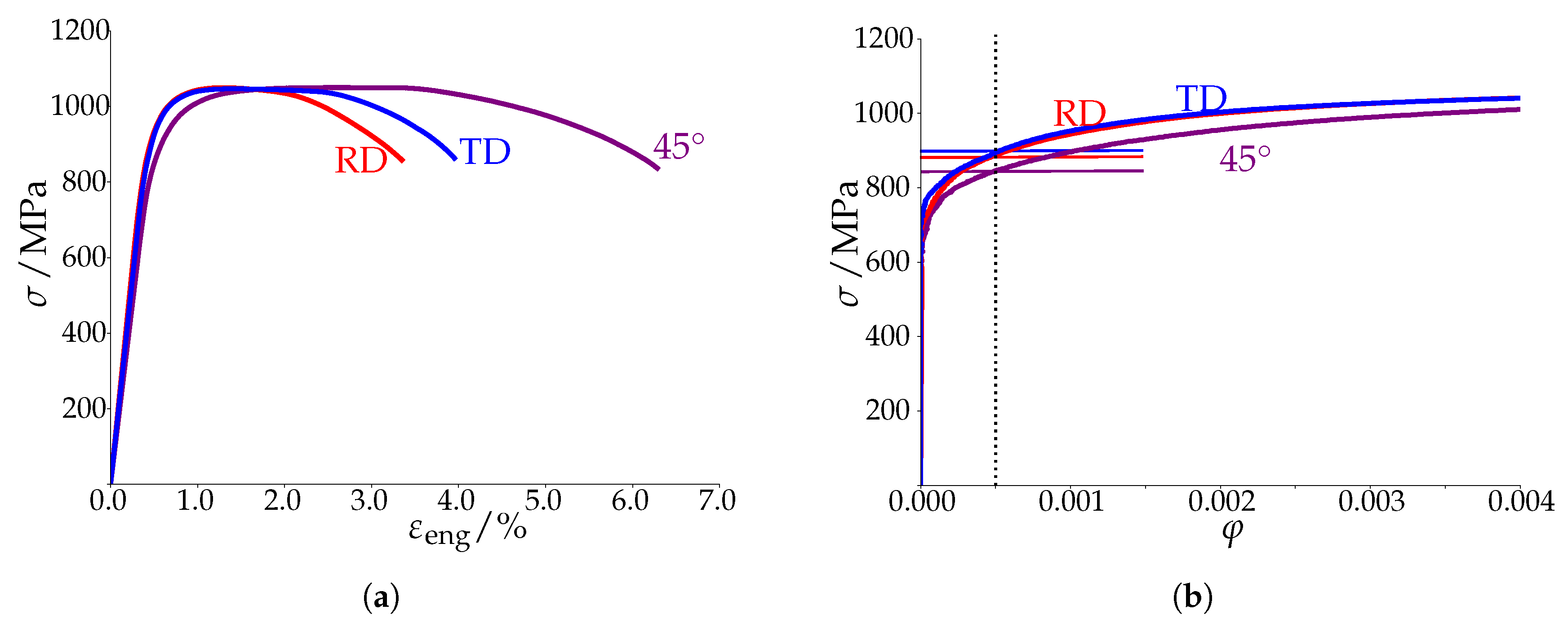
The results from the tensile tests of the three samples from the flange material (Figure 1) are given in Figure 6; Figure 6a shows the engineering stress–strain curves and Figure 6b the extracted flow curves together with the 0.05% proof stress used to approximate the yield point. A clear influence of the loading direction can be seen: the sample oriented under 45 between RD and TD shows a significantly higher uniform elongation as well as a slightly higher strain hardening rate in comparison to the samples oriented in RD and TD, respectively. To determine the yield stress from the stress–strain curve, first the elastic portion of the strain is subtracted and the flow curves are plotted (Figure 6b). Then, the stress at 0.05% plastic strain was defined as the proof stress/yield point σ y . The values determined in this manner amount to about 895 M Pa in RD, 890 M Pa in TD and 845 M Pa under 45 rotation between RD and TD.
A similar but automated procedure was employed to define the yield stress of each of the 384 crystal plasticity simulations. For the automatic determination, first a continuous representation has been created with a spline interpolation from the 25 stress–strain values per simulation. From this smooth stress–strain curve, the elastic part has been subtracted to evaluate the stress at 0.05% plastic strain. A comparison with results obtained by the method proposed by Christensen [44] and the direct calculation of a plastic strain offset from the constitutive model (i.e., the plastic strain calculated from L p ) revealed only quantitative but no qualitative differences. It should be noted that adjusting the phenomenological constitutive parameters allows to reproduce the yield point or proof stress for any other method or threshold value as well.
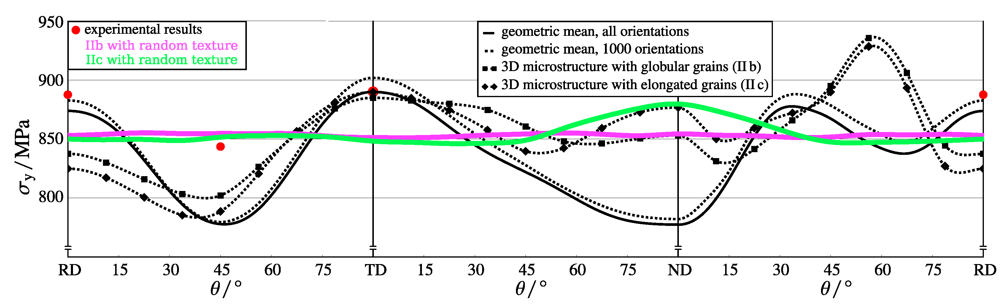
Table 3 gives an overview of the obtained yield point values for loading along ND, RD and TD. In this table, the microstructure representations used to adjust the parameters are also indicated; those are the full orientation set for the Taylor factor calculation and variant II c for the full-field simulations. An influence of both, orientation data and modeling approach, is observed:
  • The yield stress calculated for the individual sections with the analytic approach depends slightly on the data set, it differs by 30 M Pa (i.e., 3.4%) for the yield stress in TD direction σ y , TD , see Table 3a.
  • The various microstructure models used for the individual data (I a to I e) predict differences of up to 38 M Pa ( σ y , TD calculated from ND-section data), see Table 3a.
  • The yield stress in RD, σ y , RD , predicted by all simulations is lower than the value obtained from the analytic expression.
  • Sampling 1000 orientations from the combined texture results in an increase of the predicted yield stress by 4 M Pa –12 M Pa when employing the analytic approach, see Table 3b.
  • Employing the simpler models (II a: 3D microstructure without grain information and II b: 3D microstructure with globular grains) lowers σ y , TD and σ y , ND and increases σ y , RD in comparison to model II c (3D microstructure with elongated grains) which has the most realistic grain geometry, see Table 3b.
The course of σ y is presented in Figure 7 in a similar fashion as for the Young’s modulus in Figure 5. For σ y , however, only results obtained from the combined texture data are presented as the inaccuracies resulting from the use of the individual measurements are already known. It can be seen that the two considered simulation approaches (II b and II c) form a narrow band (less than 15 M Pa deviation) of yield point values and cross at four rotation angles. Although both analytic results are also close to each other, a clear difference to the simulation results can be seen. More precisely, the simulations predict a rather constant yield point from TD to ND (RD-section) and a peak between ND and RD whereas the Taylor factor calculation results in a decrease from TD to ND followed by a leveling-off increase between ND and RD. Qualitatively, the minimum at 45 between RD and TD is similarly predicted by the simulations and the analytic expression but the latter forecasts a higher value at RD. Comparison to the experimental results reveals a closer agreement for the crystal plasticity simulation at 45 between RD and TD and for the analytic expression at RD. When comparing the results of the simulations using a random texture, it can be seen that the grain morphology has only an effect when loading along ND, that is, perpendicular to the flat side of the elongated grains. More precisely, σ y of the microstructure with elongated grains is higher by approximately 40 M Pa in comparison to the microstructure having globular grains.
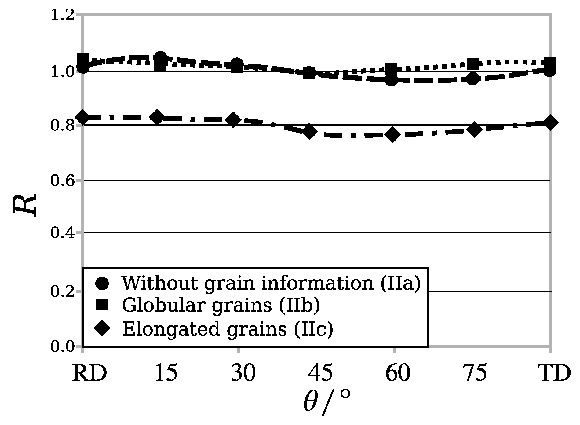
To investigate how the grain morphology influences the materials response at higher strain levels, the Lankford coefficient R, that is, the ratio between in-plane strain (perpendicular to the loading direction) and the out of plane strain (normal to the normal direction) is computed at a total strain of 10% in loading direction. Only 3D models using the combined and downsampled texture information are compared. The results are shown in Figure 8. It can be seen that the incorporation of the grain shape results in a reduced R value, while there is no significant difference whether spatially resolved globular grains or individual orientations per material point are used. It should be noted that the values of R depend critically on the used method, that is, which strain level is selected and whether the strain increments or the total strain is used for the determination.

4.2. Micro-Mechanical Behaviour

The micro-mechanical behaviour presented in the following is based on the simulation results at step 20, that is, a strain of approximately 0.04%. This strain level corresponds to a stress just below the proof stress.
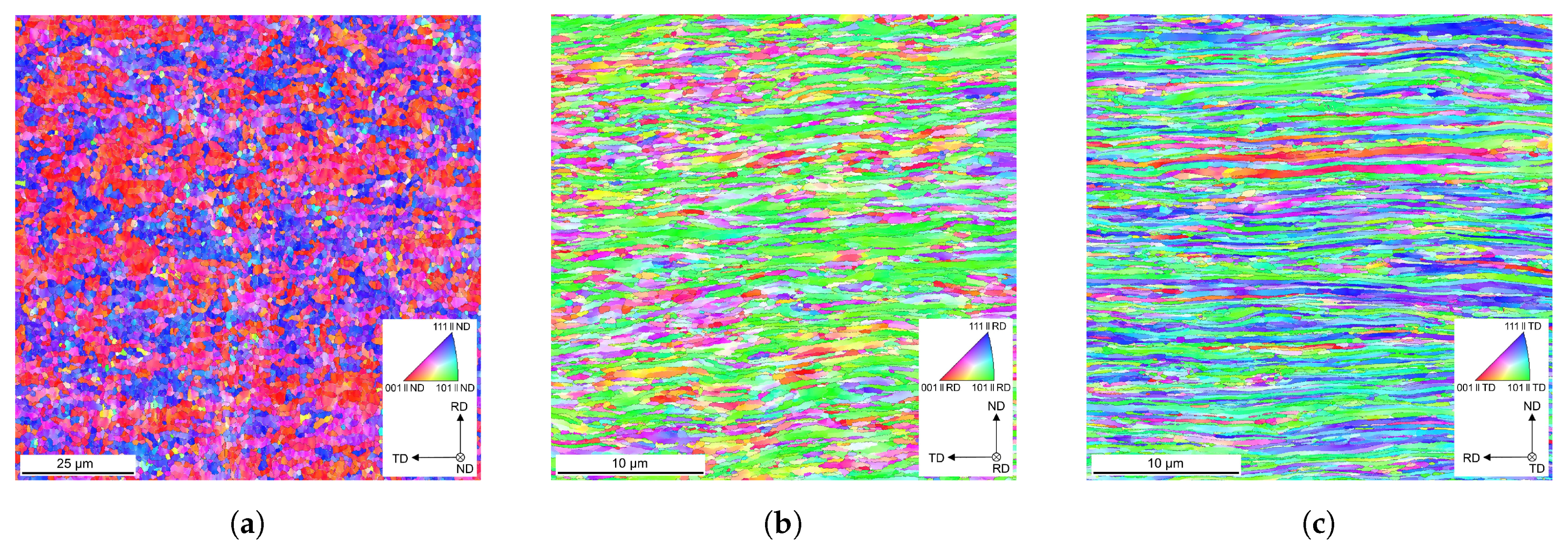
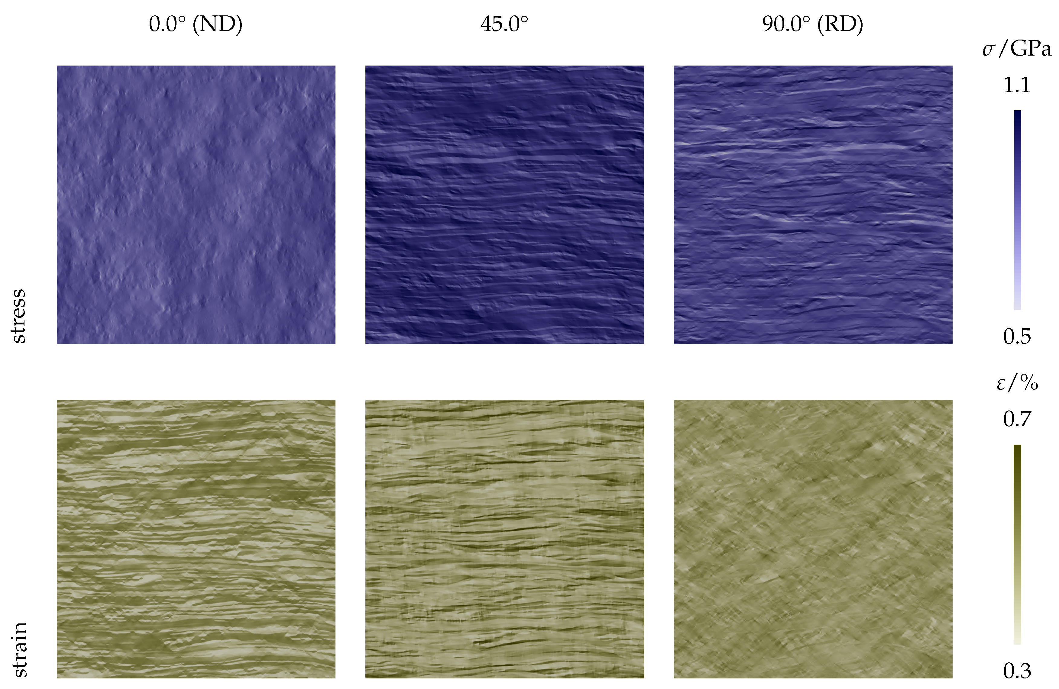
The spatial distribution of stress and strain in loading direction is shown exemplarily for the TD-section Figure 9, that is, a model of type I a. In this figure, the local stress and strain in loading direction is shown at 0.0 , 45.0 , 90.0 to ND. The grain structure is clearly visible, where the elongated grains are most obvious in the strain map when loaded perpendicular to the long grain axis and in the stress map when loaded along the long axis. A similar pattern can be observed for the RD-section (not shown in this study). The clear patterning ranging over the whole microstructure is less pronounced for equiaxed grains, that is, the ND section and 
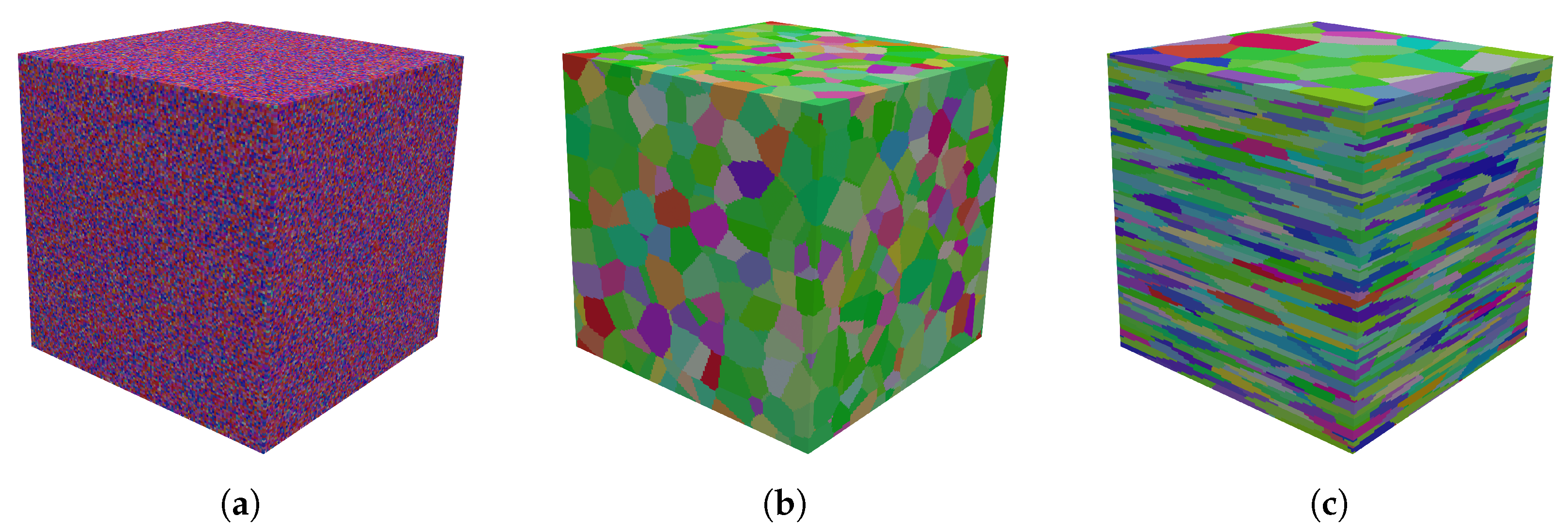
Voronoi tessellated structures with globular grain morphology in two and three dimensions (I d, I e and II b). The pattern is totally missing for the random spatial distribution of crystallographic orientations (I b, I c and II a).
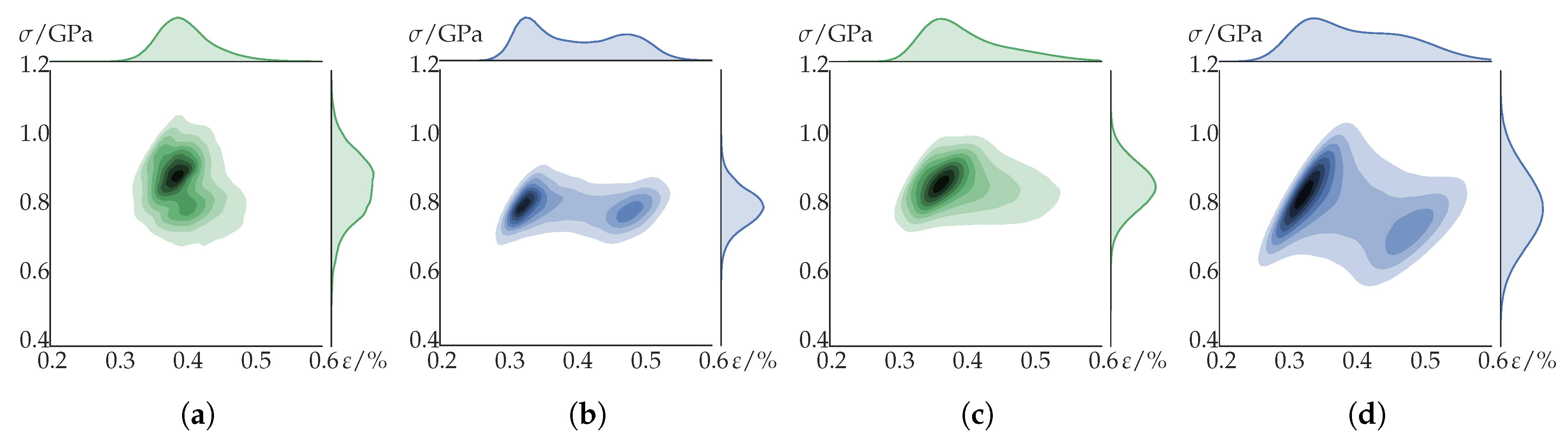
For a more quantitative inspection that also enables to systematically investigate the 3D microstructures, “heat maps” of the stress–strain response of each voxel of the employed microstructures are plotted. In Figure 10, such maps are shown for the 2D microstructure models generated from all measured crystallographic orientations in the RD-section sample (model type I a and I b). Figure 10a,c show the stress–strain response for loading along TD, that is, along the elongated grains, for the model including grain morphology and the model with random distribution, respectively. The corresponding plots for loading along ND, that is, perpendicular to the long axis of the grains are given in Figure 10b,d. Independently of the microstructure model, a characteristic unimodal distribution results from the loading along TD while a bimodal distribution results from the loading along the ND. This bimodal distribution is approximately parallel to the strain axis and, hence, results in unimodal stress distributions (shown on the right side of the heat maps). In contrast, the shape of the strain distributions (shown on the top of the heat maps) depends on the microstructure model. Taking the grain shape into account (I a, Figure 10a) results in a bimodal distribution while the minimum deteriorates to a plateau for the random orientation assignment (I b, Figure 10d).
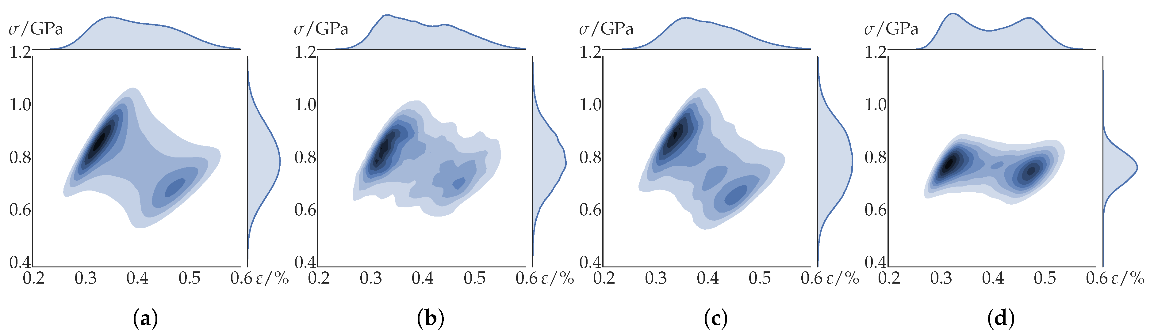
Figure 11 shows the heat maps for loading along ND from model variants I c (Random orientation assignment 3D), I d (2D Voronoi tessellation), I e (3D Voronoi tessellation) created from the RD-section and II c (i.e., using the combined texture information). Comparing Figure 11a with Figure 10d shows that for texture component modeling a difference in the stress–strain partitioning between the 2D and the 3D model (model I b and I c) is hard to ascertain. In contrast, using a 2D or a 3D model makes a difference for spatially resolved grains: The 2D variant of the model with 1000 grains (I d, Figure 11b) shows significantly stronger clustering than the 3D counterpart (I e, Figure 11c). The use of a realistic grain shape (II c, Figure 11d) narrows the strain distribution in comparison to the use of globular grains (I d, Figure 11c). The strain distribution is even more narrow when the measured microstructure is directly imported (I a, Figure 10b).

5. Discussion

Based on the results presented in the previous section, the different approaches for predicting the global and local material response from experimental orientation data are discussed here. This discussion is based mainly on the local behaviour as it allows to quantify the factors influencing the internal stress and strain distribution which in turn determines the global response.
As revealed by the micro-mechanical investigations, the stress–strain distribution resulting from the full-field simulations has a characteristic shape for the different loading directions—a bimodal distribution results from loading along ND while unimodal distributions arise from loading along TD and RD. This behaviour is vastly independent of the selected microstructure representation, i.e., all presented numerical approaches result qualitatively in a similar distribution. It can, hence, be concluded that the materials response caused by crystallographic alignment with respect to the loading direction has a much stronger influence on the stress–strain response than the grain morphology. For the small strains (0.5%) and the rather isotropic plastic behaviour assumed in this study, the elastic constants are dominating the constitutive response. The local stress–strain behaviour can therefore be explained by the spread of the Young’s modulus in the respective direction. For loading in ND, most grains have either their 〈001〉 or 〈111〉 direction aligned with the loading direction. Since these crystals directions have vastly different directional Young’s moduli of 130 G Pa and 275 G Pa , respectively; the overall Young’s modulus distribution is characterized by two peaks. In contrast, for loading in RD, most grains have either their 〈110〉 or 〈112〉 direction aligned with the loading direction. These crystallographic directions possess virtually the same directional Young’s modulus of around 210 G Pa . Thus, in RD the overall Young’s modulus distribution shows only one narrow peak. The same holds true for loading along TD, however, the spread is slightly broader in this direction due to the presence of {112}〈110〉 orientations with a directional Young’s modulus of 275 G Pa . As these characteristics of the elastic properties are fully taken into account when using the analytic expression to compute E. Therefore, this approach (Equation (1)) gives very accurate predictions and no improvement can be achieved by utilizing full-field methods that additionally consider the grain shape.
The deviations between the predictions from the different EBSD measurements have shown that the key factor for accurate predictions is the precise determination of the crystallographic texture. This usually requires probing a large volume of the material and computationally expensive simulations. However, the number of orientations required for the actual calculation can be drastically reduced by the use of an appropriate sampling strategy. Here it was shown that sampling 1000 orientations to approximate the 12,000,000 measurement points suffices to predict the Young’s modulus with an accuracy that exceeds the precision of ultrasonic measurements [19].
When predicting the plastic behaviour in terms of the yield stress, the choice of the microstructure model has a higher influence than in the elastic case. This can be attributed to the non-linear and rate-dependent plastic behaviour which is strongly influenced by the level and direction of plastic shear in the neighboring material points. These interactions are completely ignored when using the analytic expression based on the Taylor factor (Equation (2)). Hence, the observed deviations between this simple approach and the numerical predictions are to be expected. The largest deviation is seen for loading along ND, where the upper bound prediction of the analytic expression significantly exceeds the simulation results. The reason for this observation is the very inhomogeneous strain state which renders the underlying isostrain assumption of the analytic expression not suitable in this case. This holds especially for the prediction of the Lankford coefficient which is obtained at a significantly higher strain value. In contrast, the combination of a crystallographic texture with a unimodal distribution of elastic stiffness and a grain structure resembling an array of stacked disks, lead to an almost ideal isostress situation. Therefore, approaches that are not based on the isostrain assumption [45,46,47] or self-consistent approaches as introduced by Molinari et al. [48] and Lebensohn and Tomé [49] are expected to improve the prediction without relying on computationally costly full-field simulations. In that context, it should be mentioned that the increase of the yield strength for elongated grains in comparison to globular grains observed for the random texture (Figure 7) can not be explained by reasoning in terms of isostrain or isostress models. While the isostress model gives the lower bound for the elastic modulus, here a higher yield stress is observed for the more isostress-like situation of elongated grains. Analysis of the stress–strain data has shown that this is a result of the initially higher hardening rate of the microstructure with elongated grains which results in a higher proof stress for the (relatively large) offset of 0.05% strain.
Even though the full-field simulations are largely consistent among each other, the predicted yield stress for loading along RD is lower by 50 M Pa in comparison to the experimental results. One possible reason for this discrepancy is the underlying assumption of a homogeneous initial material hardening state when setting up the simulation. To investigate how far this assumption is violated, the geometrically necessary dislocations (GNDs) in the ND-section microstructure were estimated using the approach of Field et al. [50]. Based on the median of the Taylor factor for the TD (reference direction for parameter adjustment) and the RD loading directions, the average GND density for low and high Taylor factors was computed. For loading along TD, no difference in the GND density between grains with low and high M values could be found. More precisely, the difference was less than 1%. In contrast, for loading along RD, the orientations with a lower M value showed an increase of the GND density by approximately 8% (As the GND density calculation from EBSD measurements is associated with multiple sources for errors, it is discussed here only in relative terms.). This indicates that the nominally “soft” grains for loading along RD are hardened more than their “hard” counterparts and, hence, the yield stress is underestimated in the simulations due to the assumption of a homogeneous initial material behaviour.

6. Conclusions

In the present study, the viability of simple analytical texture-based models is discussed and evaluated by comparing them with different numerical microstructure models and experimental data. As the model material used is a HSLA steel processed by linear flow splitting, special attention is paid to the characteristics of this material—namely the grain morphology and the cold rolling-type crystallographic texture—and their effect on the global and local stress–strain behaviour. The obtained results lead to the following conclusions:
  • The grain morphology only has a minor impact on anisotropic elastic and plastic properties, with differences of less than 3% between microstructure based and solely texture based numerical models.
  • Statistically sufficient orientation measurements are more important than grain morphology. Even measuring 2000 grains does not ensure obtaining a representative orientation data.
  • The HybridIa method enables a significant reduction of the orientation data that is required to accurately represent the texture.
  • The simple analytic approach based on the geometric mean is suitable for estimating anisotropic elastic properties, since it yields very similar results as more complex numerical simulations.
  • The underlying isostrain assumption of the Taylor model renders it an unsuitable choice for materials consisting of non-equiaxed grains with very strong anistropic behaviour.
These results indicate that full-field simulations are not required for predicting the Young’s modulus in dependence of the orientation. Even the simple averaging scheme used in this study predict values in agreement with experiments and full field simulations. Hence, more advanced averaging schemes Hill [22], Kiewel and Fritsche [24], Kiewel et al. [51] are unlikely to give better predictions. This finding holds also to a large extend for the plastic behaviour. Moreover, as full-field crystal plasticity simulations are often based on microstructures consisting of only a few hundred grains in an attempt to minimize the computational efforts, there is a danger of using “non-representative volume elements”. Established mean-field homogenization approaches [52] such as the Grain Interaction Model (GIA) [53], the (A)LAMEL model [54], the Relaxed Grain Cluster (RGC) model [55,56] or self-consistent approaches [48,49] are, therefore, better suited as their computational performance does not require significant compromises on the number of crystallographic orientations. In many cases they also correctly predict the texture evolution after large deformation in good agreement with experimental results [49,54], a task that is especially challenging for full-field approaches due to the severe mesh deterioration. It should be noted, however, that the underlying assumptions of mean-field homogenization models make them less suited for materials with a high contrast in stiffness or strength, such as dual phase (DP) steels [57] or α + β-titanium alloys [58].

7. Outlook

The presented findings allow also to draw conclusions for the further use of crystal plasticity simulations aiming at investigating the material response at the microstructure scale. As obvious from the investigated stress–strain correlations, the use of 2D microstructures results in more pronounced localization than in corresponding 3D microstructures and—as shown by [59,60]—makes any investigation of the local environment impossible. Given the fact that 3D characterizations, i.e., serial sectioning EBSD [61] or synchrotron measurements [62] are rather costly, the creation of artificial microstructures is a good compromise that takes both aspects, crystallographic orientation and grain morphology, into account. Decisive for such approaches is the approximation of the ODF with a rather small number of distinct orientations. The HybridIa scheme by Eisenlohr and Roters [28] has shown a good performance for this task. The microtexture, however, was not taken into account in the present study. As preferential orientation relations between neighboring grains are present in most textured materials, considering the misorientation distribution function (MODF) introduced by Pospiech et al. [63] following the approach of Miodownik et al. [64] can further increase the similarity between real and synthetic microstructures. The same holds for the incorporation of in-grain orientation scatter. In the present study, the most realistic microstructure model considered only the average grain elongation. Even though this results already in a significantly improved local stress–strain response, taking the full grain size distributions into account would result in a significantly more realistic grain morphology. DREAM.3D, a software developed by Groeber et al. [65,66], Groeber and Jackson [67] provides tools for this purpose; the generated microstructures can be directly imported into DAMASK as shown by Diehl et al. [68]. Last but not least, the preexisting inhomogeneity of the hardening state among the different orientations/grains should be considered when setting up the simulation. While this is conceptually also possible with the employed phenomenological description, the use of a dislocation density-based model would allow to use directly the GND density from the EBSD measurements as an input parameter without additional fitting. The employed DAMASK package [38] offers a variety of such physics-based models for bcc materials [69], fcc steels [70] and Tungsten [71]. More advanced modeling approaches that allow to investigate in detail the influence of dislocation movement and interaction with grain boundaries [72] or the role of damage [73,74,75] are additionally available. However, the challenge remains to increase the computational performance of these models drastically before they can be employed to polycrystals that contain a sufficient number of grains to be statistically representative.

Author Contributions

Conceptualization, M.D., J.N., and E.B.; analytic calculations, J.N.; simulations, M.D.; experiments, J.N.; data curation, M.D.; writing—original draft preparation, M.D., J.N., and E.B.; writing—review and editing, M.D.; visualization, M.D.

Funding

J.N. and E.B. gratefully acknowledge the Deutsche Forschungsgemeinschaft (DFG) for founding the present work, which in part has been carried out within the Collaborative Research Centre 666 “Integral sheet metal design with higher order bifurcations—Development, Production, Evaluation”.

Conflicts of Interest

The authors declare no conflict of interest.

References

  1. Raabe, D.; Klose, P.; Engl, B.; Imlau, K.P.; Friedel, F.; Roters, F. Concepts for integrating plastic anisotropy into metal forming simulations. Adv. Eng. Mater. 2002, 4, 169–180. [Google Scholar] [CrossRef]
  2. Fritzen, F.; Böhlke, T. Three-dimensional finite element implementation of the nonuniform transformation field analysis. Int. J. Numer. Methods Eng. 2010, 84, 803–829. [Google Scholar] [CrossRef]
  3. Michel, J.C.; Suquet, P. A model-reduction approach to the micromechanical analysis of polycrystalline materials. Comput. Mech. 2016, 57, 483–508. [Google Scholar] [CrossRef]
  4. Brands, D.; Balzani, D.; Scheunemann, L.; Schröder, J.; Richter, H.; Raabe, D. Computational modeling of dual-phase steels based on representative three-dimensional microstructures obtained from EBSD data. Arch. Appl. Mech. 2016, 86, 575–598. [Google Scholar] [CrossRef]
  5. Tjahjanto, D.D.; Eisenlohr, P.; Roters, F. Multiscale deep drawing analysis of dual-phase steels using grain cluster-based RGC scheme. Model. Simul. Mater. Sci. Eng. 2015, 23, 045005. [Google Scholar] [CrossRef]
  6. Banabic, D. Sheet Metal Forming Processes; Springer: Berlin/Heidelberg, Germany, 2010. [Google Scholar] [CrossRef]
  7. Kraska, M.; Doig, M.; Tikhomirov, D.; Raabe, D.; Roters, F. Virtual material testing for stamping simulations based on polycrystal plasticity. Comput. Mater. Sci. 2009, 46, 383–392. [Google Scholar] [CrossRef]
  8. Zhang, H.; Diehl, M.; Roters, F.; Raabe, D. A virtual laboratory for initial yield surface determination using high resolution crystal plasticity simulations. Int. J. Plast. 2016, 80, 111–138. [Google Scholar] [CrossRef]
  9. Gawad, J.; Van Bael, A.; Eyckens, P.; Samaey, G.; Van Houtte, P.; Roose, D. Hierarchical multi-scale modeling of texture induced plastic anisotropy in sheet forming. Comput. Mater. Sci. 2013, 66, 65–83. [Google Scholar] [CrossRef]
  10. Roters, F.; Eisenlohr, P.; Hantcherli, L.; Tjahjanto, D.D.; Bieler, T.R.; Raabe, D. Overview of constitutive laws, kinematics, homogenization, and multiscale methods in crystal plasticity finite element modeling: Theory, experiments, applications. Acta Mater. 2010, 58, 1152–1211. [Google Scholar] [CrossRef]
  11. Marin, E.B.; Dawson, P.R. Elastoplastic finite element analyses of metal deformations using polycrystal constitutive models. Comput. Methods Appl. Mech. Eng. 1998, 165, 23–41. [Google Scholar] [CrossRef]
  12. Beaudoin, A.J.; Dawson, P.R.; Mathur, K.K.; Kocks, U.F.; Korzekwa, D.A. Application of polycrystal plasticity to sheet forming. Comput. Methods Appl. Mech. Eng. 1994, 117, 49–70. [Google Scholar] [CrossRef]
  13. Mathur, K.K.; Dawson, P.R. On modeling the development of crystallographic texture in bulk forming processes. Int. J. Plast. 1989, 5, 67–94. [Google Scholar] [CrossRef]
  14. Barbe, F.; Decker, L.; Jeulin, D.; Cailletaud, G. Intergranular and intragranular behaviour of polycrystalline aggregates. Part 1: F.E. model. Int. J. Plast. 2001, 17, 513–536. [Google Scholar] [CrossRef]
  15. Groche, P.; Vucic, D.; Jöckel, M. Basics of linear flow splitting. J. Mater. Process. Technol. 2007, 183, 249–255. [Google Scholar] [CrossRef]
  16. Groche, P.; Bruder, E.; Gramlich, S. (Eds.) Manufacturing Integrated Design; Springer International Publishing: Cham, Switzerland, 2017. [Google Scholar] [CrossRef]
  17. Bruder, E.; Ahmels, L.; Niehuesbernd, J.; Müller, C. Manufacturing-induced material properties of linear flow split and linear bend split profiles. Mater. Werkst. 2017, 48, 41–52. [Google Scholar] [CrossRef]
  18. Hölscher, M.; Raabe, D.; Lücke, K. Rolling and recrystallization textures of bcc steels. Steel Res. Int. 1991, 62, 567–575. [Google Scholar] [CrossRef]
  19. Niehuesbernd, J.; Müller, C.; Pantleon, W.; Bruder, E. Quantification of local and global elastic anisotropy in ultrafine grained gradient microstructures, produced by linear flow splitting. Mater. Sci. Eng. A 2013, 560, 273–277. [Google Scholar] [CrossRef]
  20. Voigt, W. Über die Beziehung zwischen den beiden Elastizitätskonstanten isotroper Körper. Ann. Phys. 1889, 38, 573–587. [Google Scholar] [CrossRef]
  21. Reuss, A. Berechnung der Fließgrenze von Mischkristallen auf Grund der Plastizitätsbedingung für Einkristalle. Z. Angew. Math. Mech. 1929, 9, 49–58. [Google Scholar] [CrossRef]
  22. Hill, R. The Elastic Behaviour of a Crystalline Aggregate. Proc. Phys. Soc. Sect. A 1952, 65, 349. [Google Scholar] [CrossRef]
  23. Jöchen, K.; Böhlke, T.; Fritzen, F. Influence of the Crystallographic and the Morphological Texture on the Elastic Properties of Fcc Crystal Aggregates. Solid State Phenom. 2010, 160, 83–86. [Google Scholar] [CrossRef]
  24. Kiewel, H.; Fritsche, L. Calculation of effective elastic moduli of polycrystalline materials including nontextured samples and fiber textures. Phys. Rev. B 1994, 50, 5–16. [Google Scholar] [CrossRef] [PubMed]
  25. Taylor, G.I. Plastic strain in metals. J. Inst. Met. 1938, 62, 307–324. [Google Scholar]
  26. Roters, F.; Zhao, Z. Application of the Texture Component Crystal Plasticity Finite Element Method for Deep Drawing Simulations—A Comparison with Hill’s Yield Criterion. Adv. Eng. Mater. 2002, 4, 221–223. [Google Scholar] [CrossRef]
  27. Böhlke, T.; Risy, G.; Bertram, A. A texture component model for anisotropic polycrystal plasticity. Comput. Mater. Sci. 2005, 32, 284–293. [Google Scholar] [CrossRef]
  28. Eisenlohr, P.; Roters, F. Selecting sets of discrete orientations for accurate texture reconstruction. Comput. Mater. Sci. 2008, 42, 670–678. [Google Scholar] [CrossRef]
  29. Jöchen, K.; Böhlke, T. Representative reduction of crystallographic orientation data. J. Appl. Crystallogr. 2013, 46, 960–971. [Google Scholar] [CrossRef]
  30. Bachmann, F.; Hielscher, R.; Schaeben, H. Texture Analysis with MTEX—Free and Open Source Software Toolbox. Solid State Phenom. 2010, 160, 63–68. [Google Scholar] [CrossRef]
  31. Diehl, M. High-Resolution Crystal Plasticity Simulations; Apprimus Wissenschaftsverlag: Aachen, Germany, 2016. [Google Scholar]
  32. Hutchinson, J.W. Bounds and self-consistent estimates for creep of polycrystalline materials. Proc. R. Soc. A 1976, 348, 101–127. [Google Scholar] [CrossRef]
  33. Peirce, D.; Asaro, R.J.; Needleman, A. An analysis of nonuniform and localized deformation in ductile single crystals. Acta Metall. 1982, 30, 1087–1119. [Google Scholar] [CrossRef]
  34. Rayne, J.A.; Chandrasekhar, B.S. Elastic Constants of Iron from 4.2 to 300 °K. Phys. Rev. 1961, 122, 1714–1716. [Google Scholar] [CrossRef]
  35. Adams, J.J.; Agosta, D.S.; Leisure, R.G.; Ledbetter, H. Elastic constants of monocrystal iron from 3 to 500 K. J. Appl. Phys. 2006, 100, 113530. [Google Scholar] [CrossRef]
  36. Tasan, C.C.; Hoefnagels, J.P.M.; Diehl, M.; Yan, D.; Roters, F.; Raabe, D. Strain localization and damage in dual phase steels investigated by coupled in-situ deformation experiments-crystal plasticity simulations. Int. J. Plast. 2014, 63, 198–210. [Google Scholar] [CrossRef] [Green Version]
  37. Roters, F.; Eisenlohr, P.; Kords, C.; Tjahjanto, D.D.; Diehl, M.; Raabe, D. DAMASK: The Düsseldorf Advanced Material Simulation Kit for studying crystal plasticity using an FE based or a spectral numerical solver. In Procedia IUTAM: IUTAM Symposium on Linking Scales in Computation: From Microstructure to Macroscale Properties; Cazacu, O., Ed.; Elsevier: Amsterdam, The Netherlands, 2012; Volume 3, pp. 3–10. [Google Scholar] [CrossRef] [Green Version]
  38. Roters, F.; Diehl, M.; Shanthraj, P.; Eisenlohr, P.; Reuber, C.; Wong, S.L.; Maiti, T.; Ebrahimi, A.; Hochrainer, T.; Fabritius, H.O.; et al. DAMASK—The Düsseldorf Advanced Material Simulation Kit for Modelling Multi-Physics Crystal Plasticity, Damage, and Thermal Phenomena from the Single Crystal up to the Component Scale. Comput. Mater. Sci. 2019, 158, 420–478. [Google Scholar] [CrossRef]
  39. Lahellec, N.; Michel, J.C.; Moulinec, H.; Suquet, P. Analysis of Inhomogeneous Materials at Large Strains Using Fast Fourier Transforms. In IUTAM Symposium on Computational Mechanics of Solid Materials at Large Strains; Solid Mechanics and Its Applications; Miehe, C., Ed.; Kluwer Academic Publishers: Dordrecht, The Netherlands, 2001; Volume 108, pp. 247–258. [Google Scholar] [CrossRef] [Green Version]
  40. Moulinec, H.; Suquet, P. A numerical method for computing the overall response of nonlinear composites with complex microstructure. Comput. Methods Appl. Mech. Eng. 1998, 157, 69–94. [Google Scholar] [CrossRef]
  41. Lebensohn, R.A. N-site modeling of a 3D viscoplastic polycrystal using fast Fourier transform. Acta Mater. 2001, 49, 2723–2737. [Google Scholar] [CrossRef]
  42. Eisenlohr, P.; Diehl, M.; Lebensohn, R.A.; Roters, F. A spectral method solution to crystal elasto-viscoplasticity at finite strains. Int. J. Plast. 2013, 46, 37–53. [Google Scholar] [CrossRef]
  43. Shanthraj, P.; Eisenlohr, P.; Diehl, M.; Roters, F. Numerically robust spectral methods for crystal plasticity simulations of heterogeneous materials. Int. J. Plast. 2015, 66, 31–45. [Google Scholar] [CrossRef]
  44. Christensen, R.M. Observations on the definition of yield stress. Acta Mech. 2008, 196, 239–244. [Google Scholar] [CrossRef]
  45. Sachs, G. Mitteilungen der Deutschen Materialprüfungsanstalten; Chapter Zur Ableitung einer Fließbedingung; Springer: Berlin/Heidelberg, Germany, 1929; pp. 94–97. [Google Scholar] [CrossRef]
  46. Leffers, T.; Van Houtte, P. Calculated and experimental orientation distributions of twin lamellae in rolled brass. Acta Metall. 1989, 37, 1191–1198. [Google Scholar] [CrossRef]
  47. Ahzi, S.; Asaro, R.J.; Parks, D.M. Application of crystal plasticity theory for mechanically processed BSCCO superconductors. Mech. Mater. 1993, 15, 201–222. [Google Scholar] [CrossRef]
  48. Molinari, A.; Canova, G.R.; Ahzi, S. A self-consistent approach of the large deformation polycrystal viscoplasticity. Acta Metall. 1987, 35, 2983–2994. [Google Scholar] [CrossRef]
  49. Lebensohn, R.A.; Tomé, C.N. A self-consistent anisotropic approach for the simulation of plastic deformation and texture development of polycrystals: Application to zirconium alloys. Acta Metall. Mater. 1993, 41, 2611–2624. [Google Scholar] [CrossRef]
  50. Field, D.P.; Trivedi, P.B.; Wright, S.I.; Kumar, M. Analysis of local orientation gradients in deformed single crystals. Ultramicroscopy 2005, 103, 33–39. [Google Scholar] [CrossRef]
  51. Kiewel, H.; Bunge, H.J.; Fritsche, L. Effect of the Grain Shape on the Elastic Constants of Polycrystalline Materials. Textures Microstruct. 1996, 28, 17–33. [Google Scholar] [CrossRef] [Green Version]
  52. Jöchen, K. Homogenization of the Linear and Non-linear Mechanical behaviour of Polycrystals; KIT Scientific Publishing: Karlsruhe, Germany, 2013. [Google Scholar] [CrossRef]
  53. Crumbach, M.; Pomana, G.; Wagner, P.; Gottstein, G. A Taylor Type Deformation Texture Model Considering Grain Interaction and Material Properties. Part I—Fundamentals. In Recrystallisation and Grain Growth, Proceedings of the First Joint Conference; Gottstein, G., Molodov, D.A., Eds.; Springer: Berlin, Germany, 2001; pp. 1053–1060. [Google Scholar]
  54. Van Houtte, P. Deformation texture prediction: From the Taylor model to the advanced Lamel model. Int. J. Plast. 2005, 21, 589–624. [Google Scholar] [CrossRef]
  55. Eisenlohr, P.; Tjahjanto, D.D.; Hochrainer, T.; Roters, F.; Raabe, D. Texture Prediction from a Novel Grain Cluster-Based Homogenization Scheme. Int. J. Mater. Form. 2009, 2, 523–526. [Google Scholar] [CrossRef]
  56. Tjahjanto, D.D.; Eisenlohr, P.; Roters, F. Relaxed Grain Cluster (RGC) Homogenization Scheme. Int. J. Mater. Form. 2009, 2, 939–942. [Google Scholar] [CrossRef] [Green Version]
  57. Tasan, C.C.; Diehl, M.; Yan, D.; Bechtold, M.; Roters, F.; Schemmann, L.; Zheng, C.; Peranio, N.; Ponge, D.; Koyama, M.; et al. An overview of dual-phase steels: Advances in microstructure-oriented processing and micromechanically guided design. Annu. Rev. Mater. Res. 2015, 45, 391–431. [Google Scholar] [CrossRef]
  58. Appel, F.; Wagner, R. Microstructure and deformation of two-phase γ-titanium aluminides. Mater. Sci. Eng. R Rep. 1998, 22, 187–268. [Google Scholar] [CrossRef]
  59. Zeghadi, A.; N’guyen, F.; Forest, S.; Gourgues, A.F.; Bouaziz, O. Ensemble averaging stress–strain fields in polycrystalline aggregates with a constrained surface microstructure—Part 1: Anisotropic elastic behaviour. Philos. Mag. 2007, 87, 1401–1424. [Google Scholar] [CrossRef]
  60. Zeghadi, A.; Forest, S.; Gourgues, A.F.; Bouaziz, O. Ensemble averaging stress–strain fields in polycrystalline aggregates with a constrained surface microstructure—Part 2: Crystal plasticity. Philos. Mag. 2007, 87, 1425–1446. [Google Scholar] [CrossRef]
  61. Zaefferer, S.; Wright, S.I.; Raabe, D. Three-Dimensional Orientation Microscopy in a Focused Ion Beam–Scanning Electron Microscope: A New Dimension of Microstructure Characterization. Metall. Mater. Trans. A 2008, 39, 374–389. [Google Scholar] [CrossRef] [Green Version]
  62. Wang, L.; Li, M.; Almer, J.; Bieler, T.; Barabash, R. Microstructural characterization of polycrystalline materials by synchrotron X-rays. Front. Mater. Sci. 2013, 7, 156–169. [Google Scholar] [CrossRef]
  63. Pospiech, J.; Sztwiertnia, K.; Haessner, F. The Misorientation Distribution Function. Textures Microstruct. 1986, 6, 201–215. [Google Scholar] [CrossRef] [Green Version]
  64. Miodownik, M.; Godfrey, A.W.; Holm, E.A.; Hughes, D.A. On boundary misorientation distribution functions and how to incorporate them into three-dimensional models of microstructural evolution. Acta Mater. 1999, 47, 2661–2668. [Google Scholar] [CrossRef]
  65. Groeber, M.; Ghosh, S.; Uchic, M.D.; Dimiduk, D.M. A framework for automated analysis and simulation of 3D polycrystalline microstructures. Part 1: Statistical characterization. Acta Mater. 2008, 56, 1257–1273. [Google Scholar] [CrossRef]
  66. Groeber, M.; Ghosh, S.; Uchic, M.D.; Dimiduk, D.M. A framework for automated analysis and simulation of 3D polycrystalline microstructures. Part 2: Synthetic structure generation. Acta Mater. 2008, 56, 1274–1287. [Google Scholar] [CrossRef]
  67. Groeber, M.A.; Jackson, M.A. DREAM.3D: A Digital Representation Environment for the Analysis of Microstructure in 3D. Integr. Mater. Manuf. Innov. 2014, 3, 5. [Google Scholar] [CrossRef] [Green Version]
  68. Diehl, M.; Groeber, M.; Haase, C.; Molodov, D.A.; Roters, F.; Raabe, D. Identifying Structure–Property Relationships Through DREAM.3D Representative Volume Elements and DAMASK Crystal Plasticity Simulations: An Integrated Computational Materials Engineering Approach. JOM 2017, 69, 848–855. [Google Scholar] [CrossRef] [Green Version]
  69. Ma, A.; Roters, F.; Raabe, D. A dislocation density based consitutive law for BCC materials in crystal plasticity FEM. Comput. Mater. Sci. 2007, 39, 91–95. [Google Scholar] [CrossRef]
  70. Wong, S.L.; Madivala, M.; Prahl, U.; Roters, F.; Raabe, D. A crystal plasticity model for twinning- and transformation-induced plasticity. Acta Mater. 2016, 118, 140–151. [Google Scholar] [CrossRef]
  71. Cereceda, D.; Diehl, M.; Roters, F.; Raabe, D.; Perlado, J.M.; Marian, J. Unraveling the temperature dependence of the yield strength in single-crystal tungsten using atomistically-informed crystal plasticity calculations. Int. J. Plast. 2016, 78, 242–265. [Google Scholar] [CrossRef] [Green Version]
  72. Reuber, C.; Eisenlohr, P.; Roters, F.; Raabe, D. Dislocation density distribution around an indent in single-crystalline nickel: Comparing nonlocal crystal plasticity finite element predictions with experiments. Acta Mater. 2014, 71, 333–348. [Google Scholar] [CrossRef]
  73. Shanthraj, P.; Sharma, L.; Svendsen, B.; Roters, F.; Raabe, D. A phase field model for damage in elasto-viscoplastic materials. Comput. Methods Appl. Mech. Eng. 2016, 312, 167–185. [Google Scholar] [CrossRef]
  74. Shanthraj, P.; Svendsen, B.; Sharma, L.; Roters, F.; Raabe, D. Elasto-viscoplastic phase field modelling of anisotropic cleavage fracture. J. Mech. Phys. Solids 2017, 99, 19–34. [Google Scholar] [CrossRef]
  75. Papanikolaou, S.; Thibault, J.; Woodward, C.; Shanthraj, P.; Roters, F. Brittle to Quasi-Brittle Transition and Crack Initiation Precursors in Disordered Crystals. arXiv 2017, arXiv:1707.04332v1. [Google Scholar]
Figure 1. Upper half of the double-Y-profile produced by linear flow splitting with marked positions of the tensile samples (left) and their geometry (right).
Metals 09 01252 g001
Figure 2. Microstructure maps in three mutually perpendicular directions of the material after linear flow splitting. Crystallographic orientation is given in terms of the inverse pole figure parallel to the measurement direction. Note the lower magnification of the normal direction (ND)-section in comparison to the rolling direction (RD)- and transverse direction (TD)-section. (a) ND-section. (b) RD-section. (c) TD-section.
Metals 09 01252 g002
Figure 3. φ 2 -section of the orientation distribution function (ODF) calculated from the TD-section using a harmonic series expansion approach. φ 1 , Φ and φ 2 are the BungeEuler angles.
Metals 09 01252 g003
Figure 4. Microstructural models created from the measured crystallographic orientation. ND is aligned with the vertical direction, morphologically there is no difference between RD and TD for all three models. (a) Microstructure I c: Point-wise random orientation distribution, exemplarily shown for the ND-section. The legend is shown in Figure 2a. (b) Microstructure I e: 1000 globular grains with homogeneous crystallographic orientation, exemplarily shown for the RD-section. The legend is shown in Figure 2b. (c) Microstructure II c: 1000 elongated grains with homogeneous crystallographic orientation. The legend is shown in Figure 2c.
Metals 09 01252 g004
Figure 5. YOUNG’s modulus in dependence of loading direction. Left: ND-section, Center: RD-section, Right: TD-section. (a) Results from simulations and the geometric mean calculation using the data of the individual measurements. The range between highest and lowest simulation result from all five microstructure variants (model I a to I e) is indicated by the background color (b) Results from the simulations and the geometric mean calculations using the combined texture data.
Metals 09 01252 g005
Figure 6. Experimental results of the tensile tests from the samples cut from the flange material. (a) Engineering stress–strain curves. (b) Flow curves the with 0.05% proof stress indicated. φ: Plastic deformation.
Metals 09 01252 g006
Figure 7. Yield point in dependence of loading direction. Left: ND-section, Center: RD-section, Right: TD-section. Results from the combined simulations obtained from the individual measurements and from the geometric mean calculations.
Metals 09 01252 g007
Figure 8. Lankford coefficient in dependence of the loading direction in the ND section. Results for the 3D models using the combined texture information (II a–c) are shown.
Metals 09 01252 g008
Figure 9. Stress (top row) and strain (bottom row) in loading direction for the TD-section (direct takeover, microstructure representation I a). The left image shows loading along ND (vertical direction), the right image loading along RD (horizontal direction) and the central loading aligned at Θ = 45 in-between ND and RD. A logarithmic mapping from value to color is employed for stress and strain.
Metals 09 01252 g009
Figure 10. Distribution of the stress–strain correlation (“heat map”) in models created from all crystallographic orientations measured in the RD-section for loading along TD and ND using a kernel density estimation. Note: Modeling the response by an isostrain assumption would result in a vertical line, the isostress assumption would result in an horizontal line. (a) Direct takeover 2D (I a), loading along TD. (b) Direct takeover 2D (I a), loading along ND. (c) Random orientation assignment 2D (I b), loading along TD. (d) Random orientation assignment 2D (I b), loading along ND.
Metals 09 01252 g010
Figure 11. Distribution of the stress–strain correlation (“heat map”) in models created from the measurement in the RD-section and in a model created from the combination of all three measurements for loading along ND using a kernel density estimation. Note: Modeling the response by an isostrain assumption would result in a vertical line, the isostress assumption would result in an horizontal line. (a) Random orientation assignment 3D (I c), created from the RD-section. (b) 2D VORONOI tessellation (I d), created from the RD-section. (c) 3D VORONOI tessellation (I e), created from the RD-section. (d) 3D model with elongated grains (II c).
Metals 09 01252 g011
Table 1. Constitutive parameters for the phenomenological crystal plasticity description. (a) Elastic behaviour. (b) Plastic behaviour.
(a)
PropertyValueUnit
C 11 230 G Pa
C 12 134 G Pa
C 44 116 G Pa
(b)
PropertyValueUnit
γ ˙ 0 1.0 m m / s
τ 0 , { 110 } 354 M Pa
τ , { 110 } 837 M Pa
τ 0 , { 112 } 361 M Pa
τ , { 112 } 1538 M Pa
h 0 1.0 G Pa
Coplanar h α β 1.0
Non-coplanar h α β 1.4
n20.0
a2.0
Table 2. Young’s modulus E along ND, RD and TD. Niehuesbernd et al. [19] determined E ND = ( 204 ± 10 ) G Pa , E RD = ( 212 ± 10 ) G Pa and  E TD = ( 232 ± 10 ) G Pa by ultrasonic measurements. (a) Results from the geometric mean calculation using the texture of the individual measurements. The highest and lowest values from simulations I a (direct takeover 2D), I b (random orientation assignment 2D), I c (random orientation assignment 3D), I d (2D Voronoi tessellation) and I e (3D Voronoi tessellation) are given as superscript and subscript, respectively. (b) Results from the geometric mean calculation and from simulations using the combined texture information. II a: 3D microstructure without grain information, II b: 3D microstructure with globular grains, II c: 3D microstructure with elongated grains.
(a)
ND-SectionRD-SectionTD-Section
E ND / G Pa - 205 202 206 194 191 195
E RD / G Pa 217 219 220 - 215 214 217
E TD / G Pa 233 234 237 231 231 235 -
(b)
Geometric MeanSimulation
All Orientations1000 OrientationsII aII bII c
E ND / G Pa 198198199198196
E RD / G Pa 215215216216215
E TD / G Pa 233234235234236
Table 3. Yield stress σ y along ND, RD and TD. The experimental values are σ y , RD = 895 M Pa and σ y , TD = 890 M Pa . (a) Results from the geometric mean calculation using the texture of the individual measurements. The highest and lowest values from simulations I a (direct takeover 2D), I b (random orientation assignment 2D), I c (random orientation assignment 3D), I d (2D Voronoi tessellation) and I e (3D Voronoi tessellation) are given as superscript and subscript, respectively. (b) Results from the geometric mean calculation and simulations using the combined texture information. II a: 3D microstructure without grain information, II b: 3D microstructure with globular grains, II c: 3D microstructure with elongated grains. The results used to determine the scaling factor for the analytic expression and the crystal plasticity parameters from the experimental reference value are underlined.
(a)
ND-SectionRD-SectionTD-Section
σ y , ND / M Pa - 786 876 902 769 832 862
σ y , RD / M Pa 889 844 873 - 873 818 837
σ y , TD / M Pa 904 873 911 874 885 898 -
(b)
Geometric MeanSimulation
All Orientations1000 OrientationsII aII bII c
σ y , ND / M Pa 778782857853877
σ y , RD / M Pa 874883842837825
σ y , TD / M Pa 890902888885890

