Determination of Directional Residual Stresses by the Contour Method

Abstract

This study evaluated residual stresses in heat-treated specimens made of 316L stainless steel using FE analysis and compared them with stresses determined by the contour method. Contour method is usually used just for evaluation of residual stresses that are normal to the cut plan. In the current study this approach is extended and both normal and tangential stresses are determined. The specimens were cut using wire electrical discharge machine and the contours of the cut were measured using a coordinate measuring machine. The prior treatment of the specimens was simulated using the finite-element method. An appropriate boundary condition and temperature-dependent material model were employed. The finite-element model was validated against neutron-diffraction measurement data. The results showed a good agreement in normal and tangential directions of stress.

1. Introduction

Residual stresses have significant impact on engineering components during manufacturing and during service operation and afterwards, reducing the component life. The levels of residual stress upon heat treatment are often unknown. If they were known, qualitative characteristics of products could be predicted much more reliably. Residual stresses can be determined indirectly from elastic strains or other quantities, such as magnetic field or speed of sound [1,2]. X-ray or neutron beam diffraction can be used for this purpose as well. Another possibility is application or the conventional computational approach [3] that relies on the finite-element method (FEM) implemented in a suitable software tool. An engineer who chooses this approach faces several difficulties, the major one being associated with finding the dependence of material properties on temperature, and identifying microstructural phases that form during heat treatment. Furthermore, there is a problem with finding the value of the heat transfer coefficient. This leads to simplification and compromises because acquiring materials data and determining boundary conditions is rather demanding and expensive.

An important distinction is made between destructive and non-destructive measuring techniques for residual stresses with additional consideration of depths to which they are applicable. More information on these aspects can be found in [1].

The contour method [4,5,6] is a destructive procedure which evaluates elastic strain and normal stress field along a cut plane made through a component ranging in size from ten to hundreds of millimeters. The principle is shown schematically in Figure 1.

A part in which residual stress is to be evaluated, Figure 1a, is cut. Normal and tangential components of the released stress cause the cut surface to deform as the example in Figure 1b shows. Both cut surfaces are then measured by a 3D scanning instrument and the readings are averaged and inverted. The processed contour is imposed as a boundary condition on the cut plane of a linear elastic FE model, as shown in Figure 1c. The calculated stress required for the deformed surface to return the nominal shape represents the actual residual stress in the part.

The output from the contour method is a distribution of normal stress along the cut plane. The measurement of the surface contour only provides information about normal stress because transverse displacements are impossible to measure. However, assuming that the normal displacements are significantly larger than the transverse ones, one can also use the contour method to estimate the transverse stresses.

Our aim was to study residual stresses induced by quenching. Quenching is often used to produce the desired mechanical properties in the surface, namely stress distribution, to control the potential for fracture initiation. According to the latest findings, fracture initiation is driven by triaxiality [7] which reflects the whole stress tensor at a specific point. An ability to derive the stresses traverse to cut plane is the main advantage of the solution proposed in this paper, which extends the applicability of the standard contour method.

In this study, the contour method was employed to determine residual stresses in cylindrical specimens of 316L stainless steel. The material was chosen on purpose, as it contains only a single phase during heat treatment – which makes the computational verification relatively simple. To induce residual stresses in the material, the specimens were heated to $850{}^{\circ }$C and then rapidly cooled with water sprays.

Cuts for the contour method measurement were made along planes of symmetry in specimens as well as other planes [8]. A variation from the conventional practice consisted of the specimen clamping arrangement for wire electrical discharge machine (EDM) cutting. The specimens were only clamped on one side [9,10] to explore the viability of this convenient configuration. The shapes of the cut planes were subsequently measured using a coordinate measuring machine (CMM). Based on the measured contours, the distribution of residual stresses upon heat treatment were calculated using 3D FE linear elastic analysis.

3D FE simulation of the heat treatment was performed. The stress distribution computed in this manner was compared with the data from neutron-diffraction [11], which was chosen as a reference method, and a very good agreement was found. In addition, a FE simulation of the contour cut method was performed and results were compared with FE simulation of the heat treatment process. The stress distributions for both are comparable and in good agreement.

2. Materials and Methods

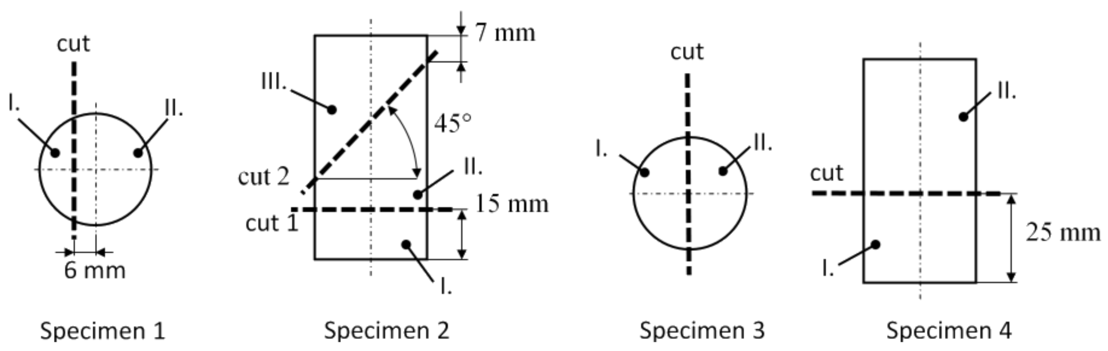
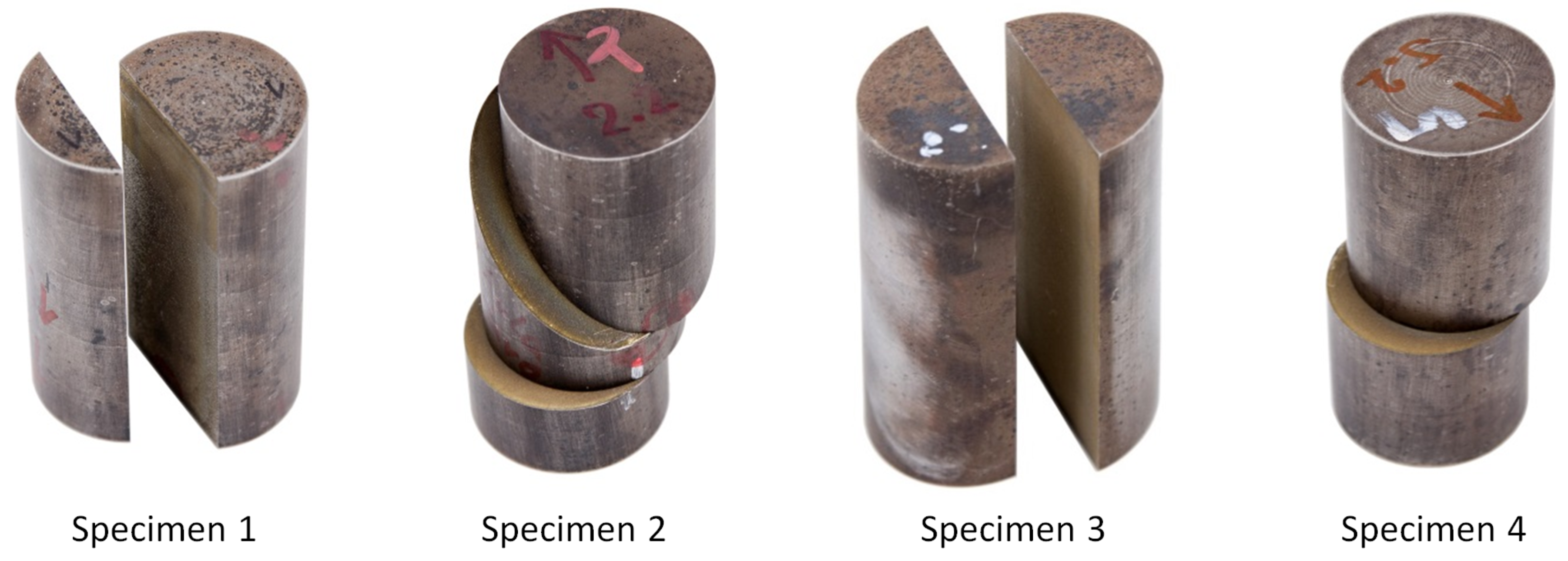
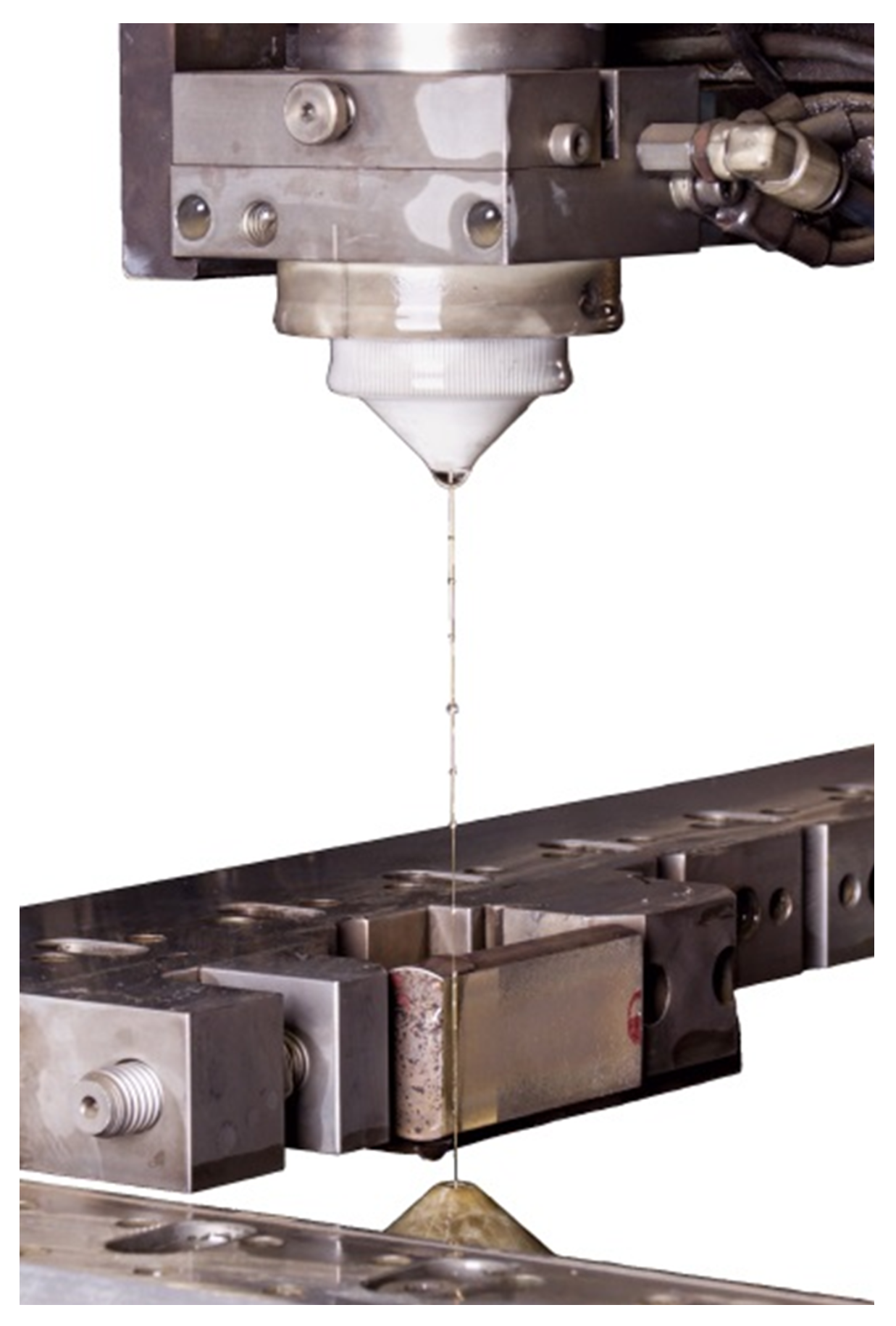
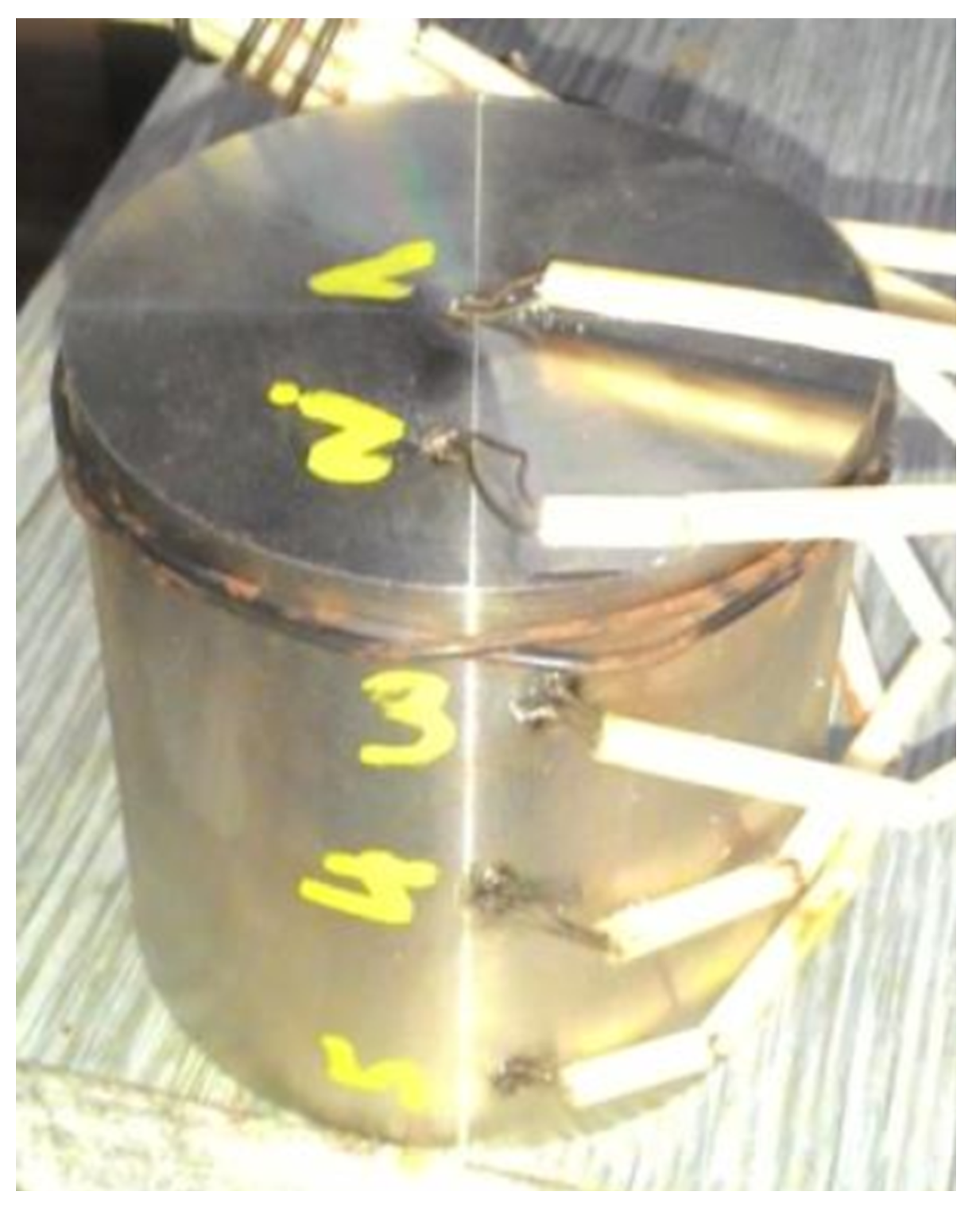
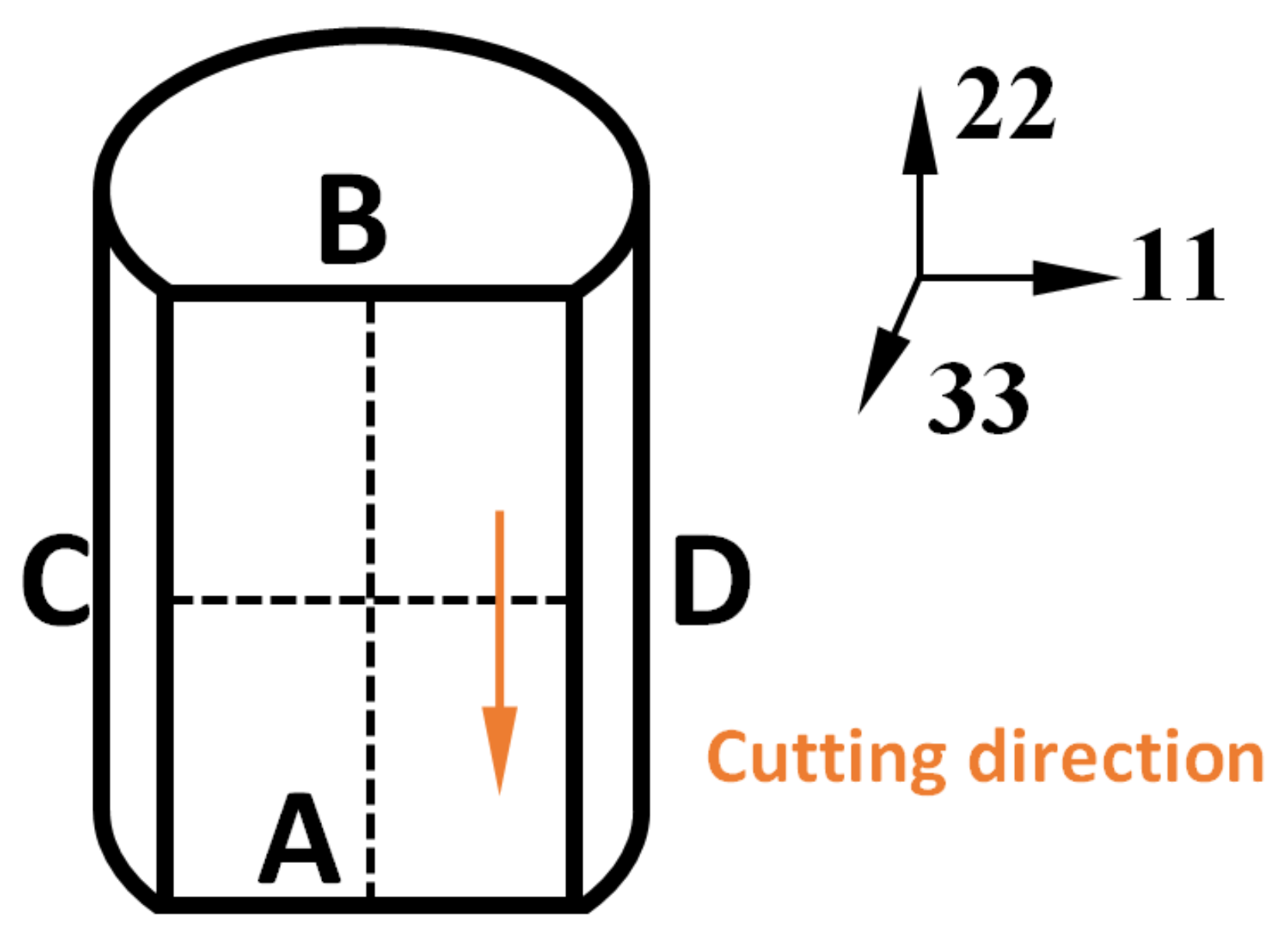
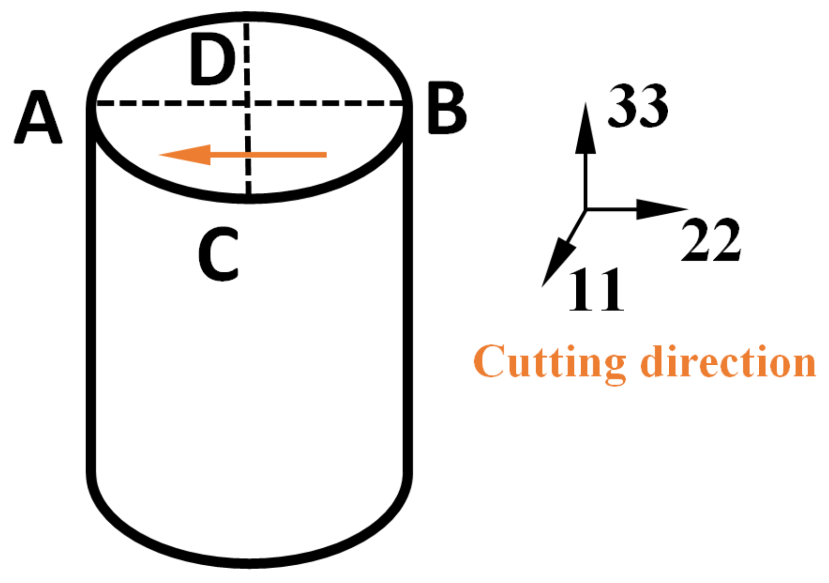
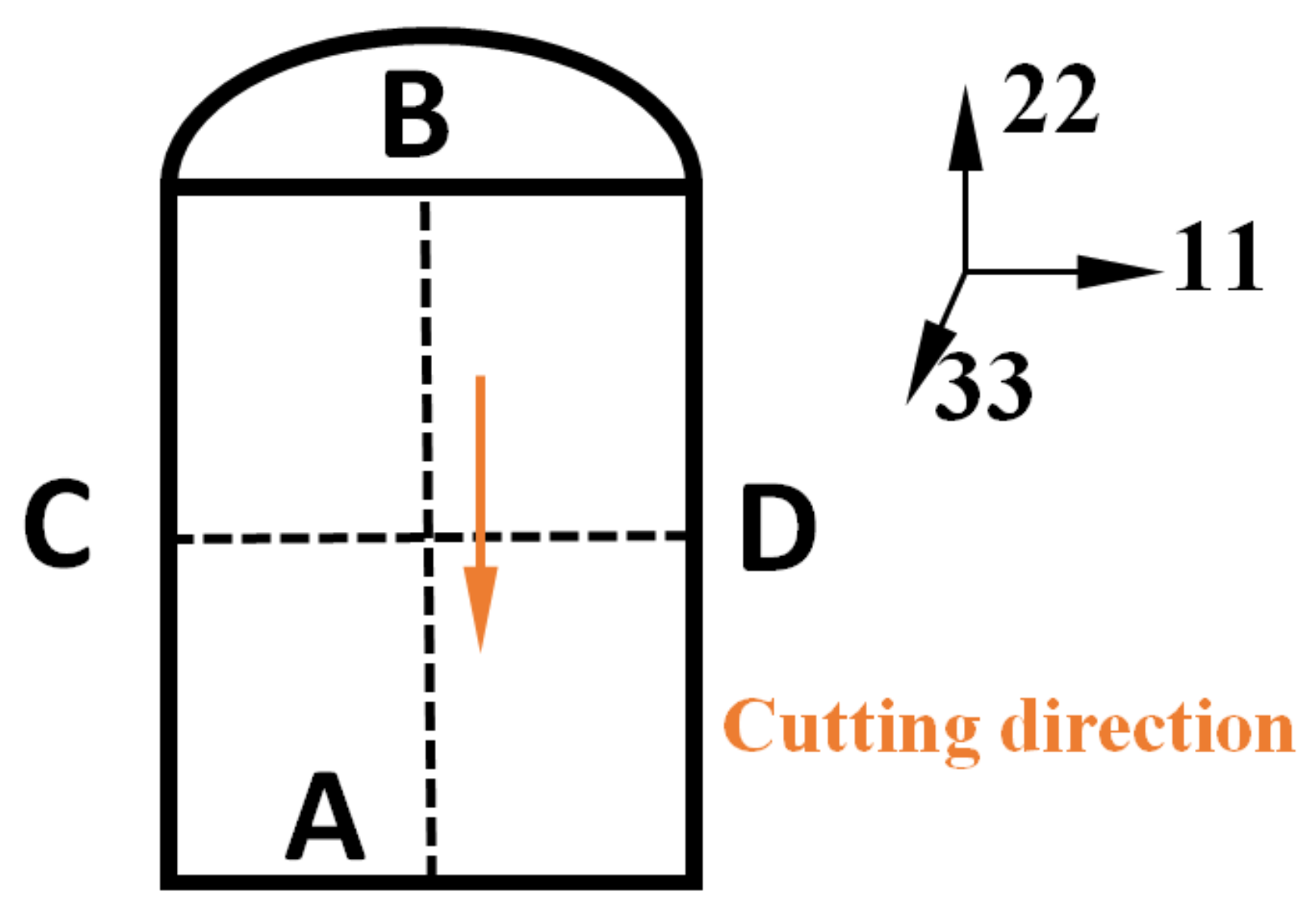
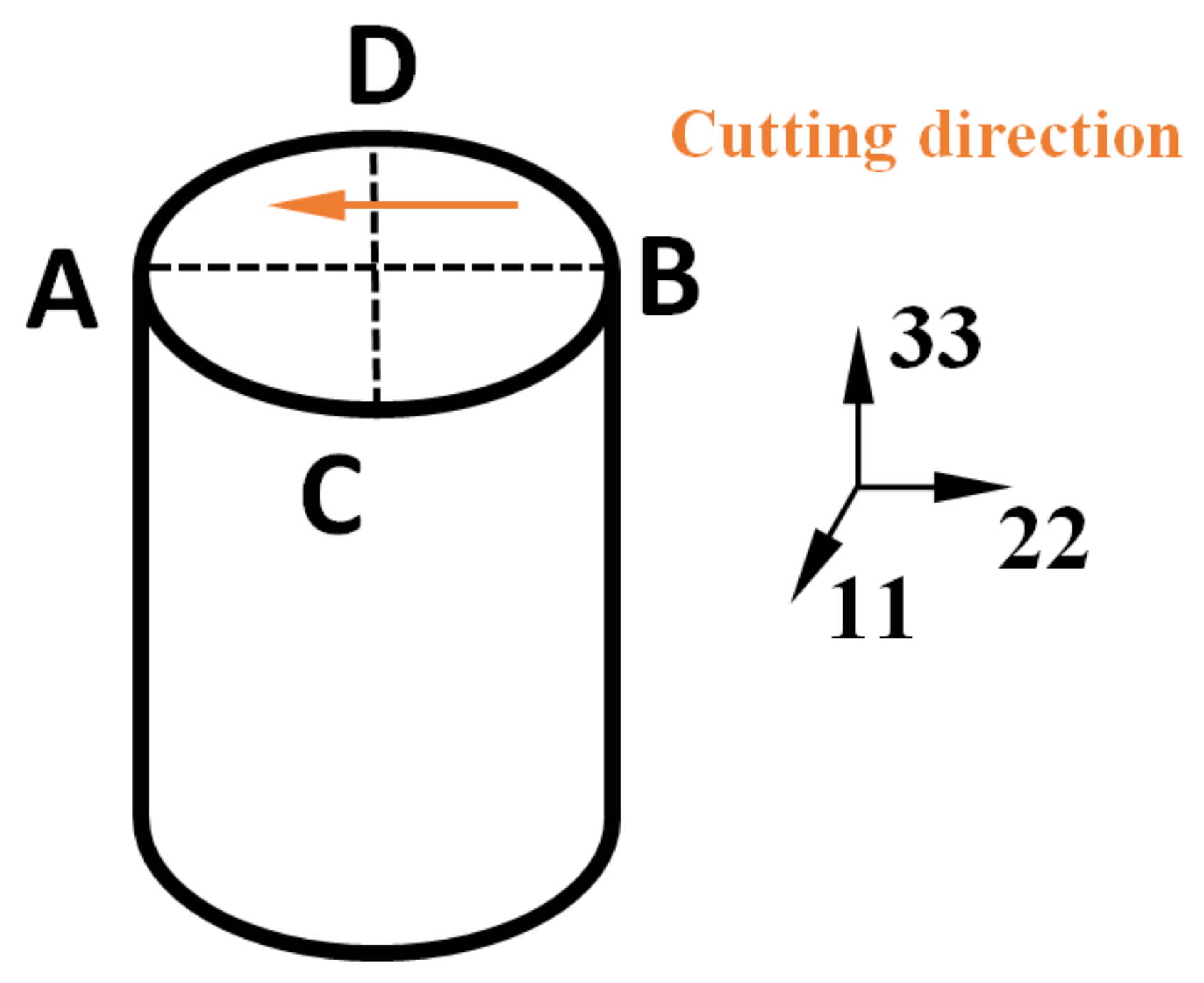
2.1. Specimen Preparation and Contour Method

Cylindrical specimens of diameter 30 mm in and height of 60 mm made of 316L steel were heat-treated and examined using the contour method. Their chemical composition was measured using a Bruker Q4 TASMAN optical emission spectrometer, providing the values listed in

Table 1. Measured chemical composition of 316L steel $[wt\%]$.

C	Si	Mn	Cr	Mo	Ni	Cu	Fe
0.021	0.534	1.335	16.66	2.003	10.447	0.489	Bal.

.

Five specimens were heated from $20{}^{\circ }$C to 850${}^{\circ }$C over 2.5 h, held for 30 min in a furnace at 850${}^{\circ }$C, Figure 2, and then quenched by several water sprays for 60 s, Figure 3. The water spray nozzles were arranged to provide symmetric cooling. At the end of this procedure, the measured temperature of the specimens was 40${}^{\circ }$C.

Four specimens were used for the contour method and one for neutron-diffraction analysis. Wire EDM cutting using a 0.25 mm-diameter wire was carried out according to the cut-up plan indicated in Figure 4 (the cut planes are indicated with dashed lines). It involved making a symmetric cut (Specimen 3), non-symmetric cuts (Specimens 1, 2 and 4) and two cuts in a single specimen (Specimen 2).

Photographs of the cut-up specimens are shown in Figure 5.

Guidelines for handling contour method specimens are discussed in [5]. In the present study, the specimens were only clamped on one side for cutting, contrary to the conventional practice, where both sides are clamped. The purpose of this modification was to simplify the handling of specimens and to reduce the risk of wire breakage. Figure 6 shows the clamping arrangement for specimen 1. The other specimens were clamped in a similar fashion.

Two cuts were made in specimen 2. The first one was perpendicular to the axis of the cylinder, as shown in Figure 4b. After the surfaces of cut 1 had been measured, the second cut was made in specimen 2 at the angle of 45${}^{\circ }$ to the axis.

Residual stresses released by cutting resulted in deformation of the cut surfaces. In each case, the displacements on both cut surfaces were measured using a Mitutoyo CMM with the Renishaw PH10T measuring head. The measurement grid was $1\times 1$ mm and the measurement precision was 0.5 $\mathsf{\mu }$m. The data was processed with a user script based on spline approximation in the Octave environment [12]. The displacements were averaged, and the contour data were smoothed to remove the appreciable noise from the signal. Figure 7 and Figure 8 show the measured displacements on two cut surfaces in specimen 1. The readily apparent differences between these surfaces are due to asymmetry of the resulting parts, the single-end clamping and the different responses to released residual stresses in each cut part. These findings agree with [9], where residual stresses were evaluated in a specimen which had been clamped in a similar manner. The effects of clamping were explored in [9] and, in great detail in [10], where cutting-induced plasticity was found to affects the residual stress data.

Summation, inversion and smoothing of the data yielded a boundary condition for FE analysis. The data from specimen 1 processed in this manner are plotted in Figure 9.

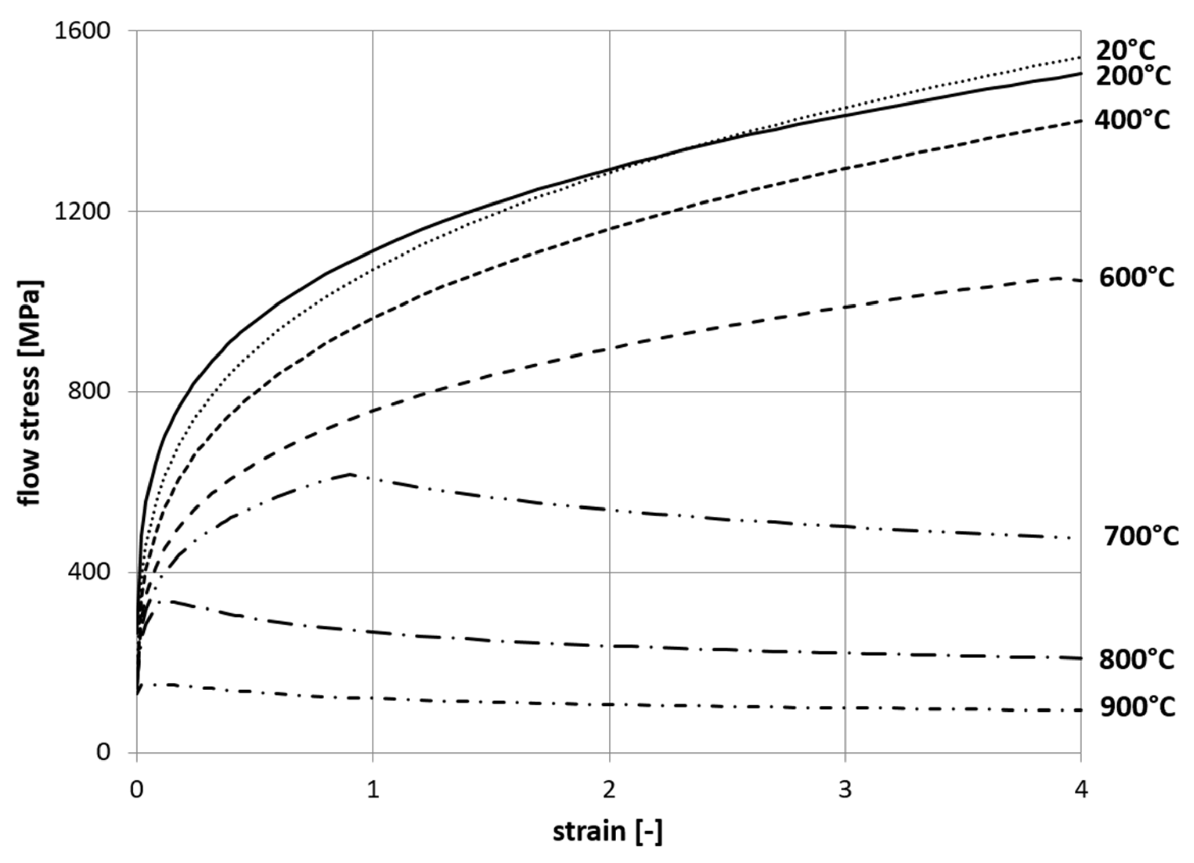
2.2. Determination of Thermo-Physical Properties

JMatPro [13] was used for computing material characteristics from the chemical composition given in Table 1. The resulting values used in this study are listed in

Table 2. Specimen 1 data after summation, inversion and smoothing.

Temperature [${}^{\circ }$C]	25	100	300	600	900
Property
Thermal conductivity [W/mK]	14.57	15.58	18.24	22.20	26.14
Specific heat [J/kgK]	455.37	475.11	508.96	549.63	621.17
Poisson’s ratio [-]	0.298	0.301	0.31	0.324	0.338
Young’s modulus [MPa]	192.96	187.74	173.39	150.78	126.69
Thermal expansivity 10-5 [1/K]	1.78	1.80	1.84	1.91	1.99

.

Flow stress curves were generated using JmatPro as a set of temperature-dependent functions [14]. Those for the strain rate $\dot{\epsilon }=0.0001{\mathrm{s}}^{-1}$ and for the temperature range from 20${}^{\circ }$C to 900${}^{\circ }$C are plotted in Figure 10. Flow stress curves for higher strain rates were similar to those shown in Figure 10.

2.3. Finite-Element Model for the Contour Method

The FE models of specimens were established as 3D linear elastic models using MSC MARC software [15]. The processed contours from physical measurement of cut specimens were applied as displacement boundary conditions. The mesh comprised eight-node brick elements with trilinear interpolation (class 5, element id 7). The characteristic length of the elements was about 1 mm. Young’s modulus and Poisson’s ratio were considered to be constants at 25${}^{\circ }$C given in Table 2.

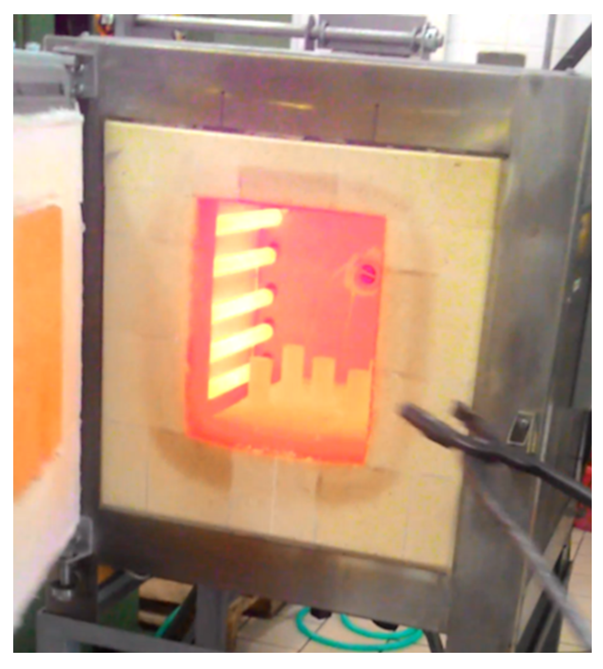
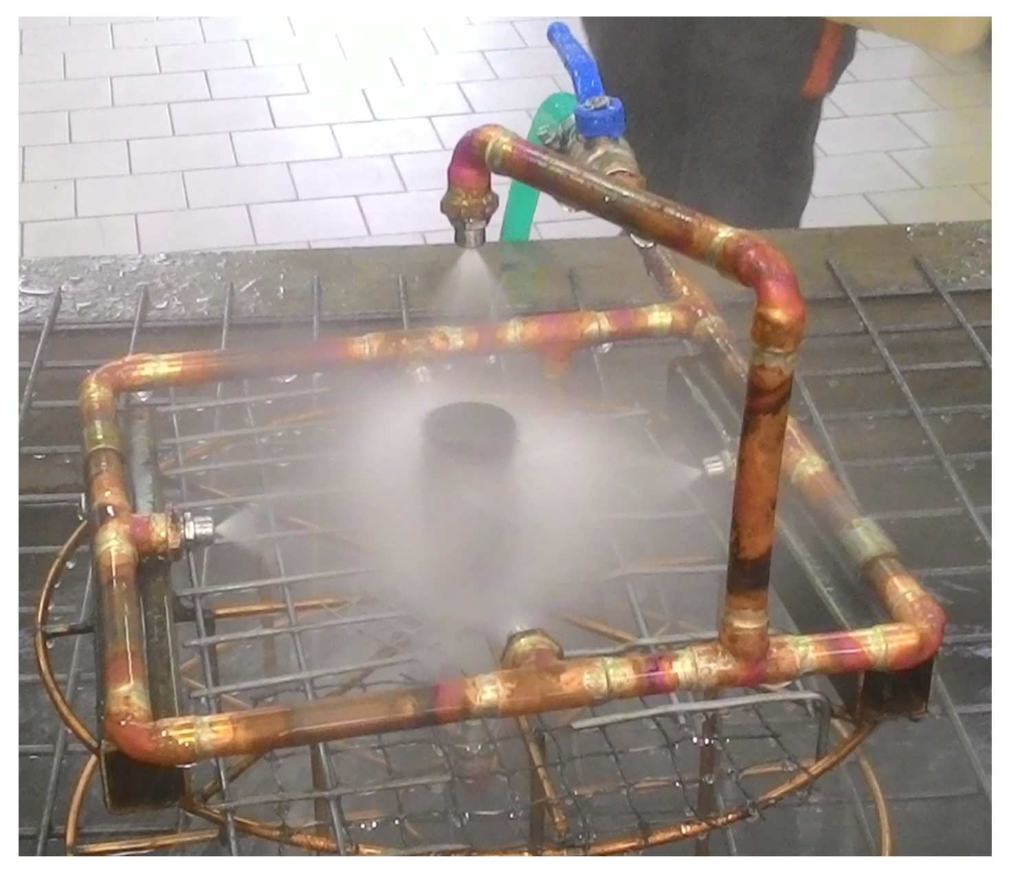
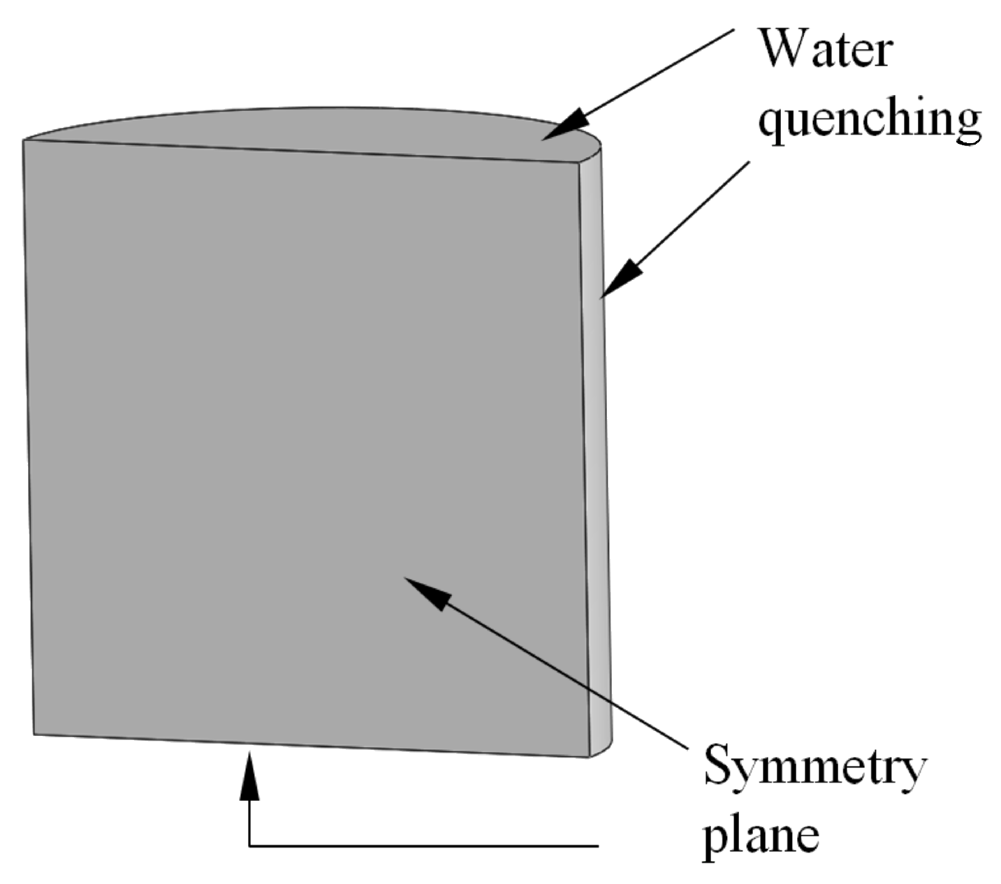
2.4. Finite-Element Model of Heat Treatment

The FE model of heat treatment was developed as a 3D problem using the MSC MARC software [15]. Since the specimens were symmetric, only one quarter of the specimen was considered, as shown in Figure 11. The mesh elements were of the same type as in the contour method model. The specimen model for heat treatment simulation consisted of 468,800 elements with a 0.25 mm characteristic length. Finer mesh elements were applied around the surfaces quenched with water.

The heat transfer coefficient (HTC) was considered to be temperature-independent, $\alpha =2000{\mathrm{W}/\mathrm{m}}^2$K. This value was derived from temperature data acquired during heat treatment using the setup shown Figure 12 and processed by inverse analysis.

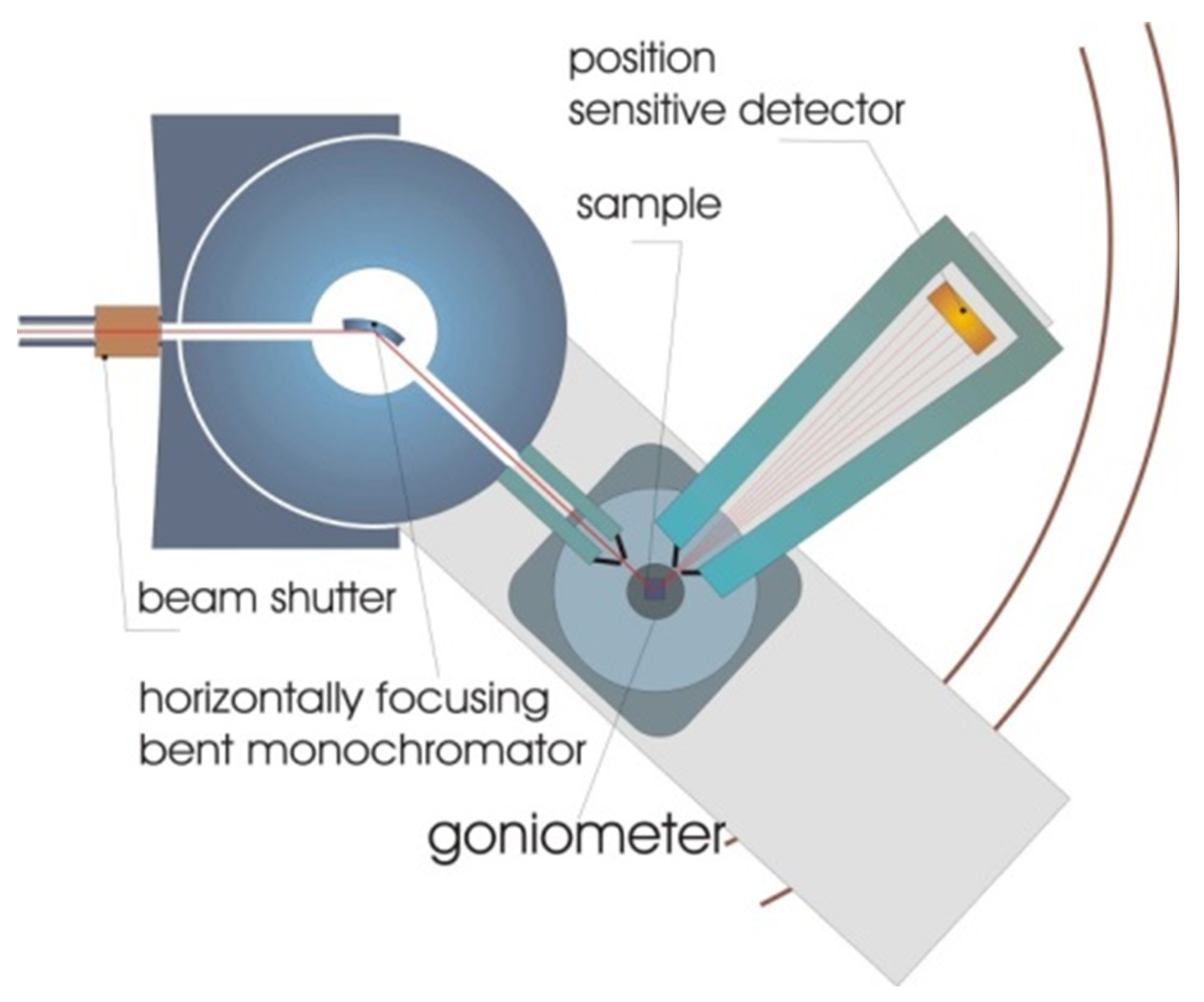
2.5. Neutron-Diffraction Measurement of Residual Stresses

The measurement was performed using the SPN-100 neutron diffractometer installed at the research reactor LVR-15 in a research center in Řež in the Czech Republic. This experimental facility is dedicated to mapping residual stresses in polycrystalline materials. The SPN-100 instrument is equipped with a curved Si monochromator and with a position-sensitive detector for fast recording of diffraction profiles. A schematic sketch of the instrument is shown in Figure 13.

Measurements were taken along three planes in the sample. The upper, central and bottom planes were located at 15, 30 and 45 mm, respectively, above the cylindrical specimen base. On each plane, measurements were taken along three directions N1, N2 and N3 spaced at 120${}^{\circ }$. Residual deformations in radial, hoop and axial directions were determined for each measured point. The procedure is illustrated schematically in Figure 14. Deformation values were thus mapped at 135 points.

The quantity measured by diffraction is a lattice strain component. Stress tensor components can be determined using Hooke’s law. The formula for calculating stress components from diffraction data is as follows [11]:

$${\sigma }_x=\frac{E_{hkl}}{(1-2v_{hkl})(1+{\nu }_{hkl})}[(1-{\nu }_{hkl}){\epsilon }_x^{hkl}+{\nu }_{hkl}({\epsilon }_y^{hkl}+{\epsilon }_z^{hkl})]$$

where ${\epsilon }_{x,y,z}^{hkl}$ is the x, y, z-component of the lattice strain measured at the $hkl$ crystal lattice plane, and E${}_{hkl}$ and ${\nu }_{hkl}$ are the values of Young’s modulus and Poisson’s ratio derived from the diffraction data, respectively. The ${\epsilon }_{x,y,z}^{hkl}$ components are measured using neutron diffraction. The corresponding relations for y and z stress components are obtained by simple permutations of x, z and y indexes. Material properties were considered to be isotropic constants at 25 ${}^{\circ }$C (Table 2).

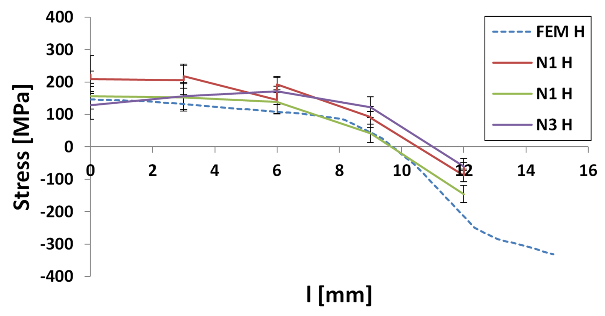
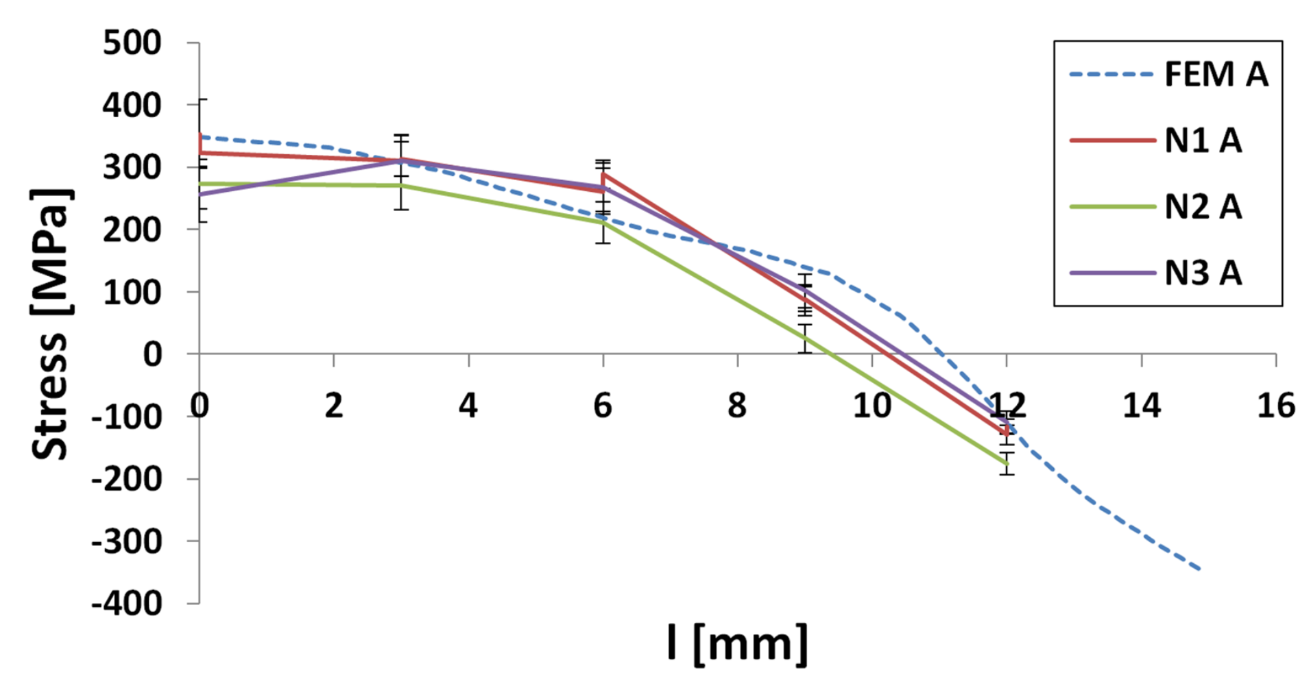
2.6. Comparison of Residual Stresses Computed from Neutron-Diffraction Measurements and Residual Stresses from the FE Model of Heat Treatment

Plots of these stresses are shown in Figure 15, Figure 16 and Figure 17 where N1-N3 means neutron measurements directions. Only the stresses on the central plane are shown because those on the upper and bottom planes had the same character.

The calculated hoop stress (Figure 16) and axial stress (Figure 17) values are in good agreement with the data from the neutron-diffraction analysis. The calculated radial stresses (Figure 15) are lower than the measured ones but the profiles are nearly identical. This comparison suggests that FE calculations of residual stress are sufficiently accurate for this type of heat treatment and could be used as a reference for further evaluation of contour cuts.

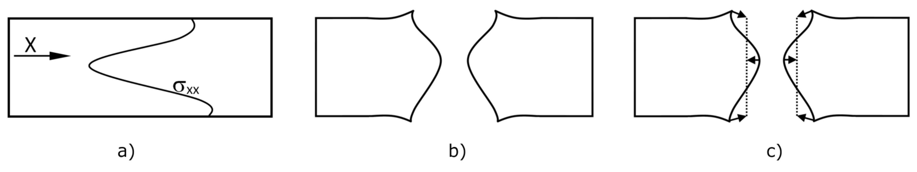
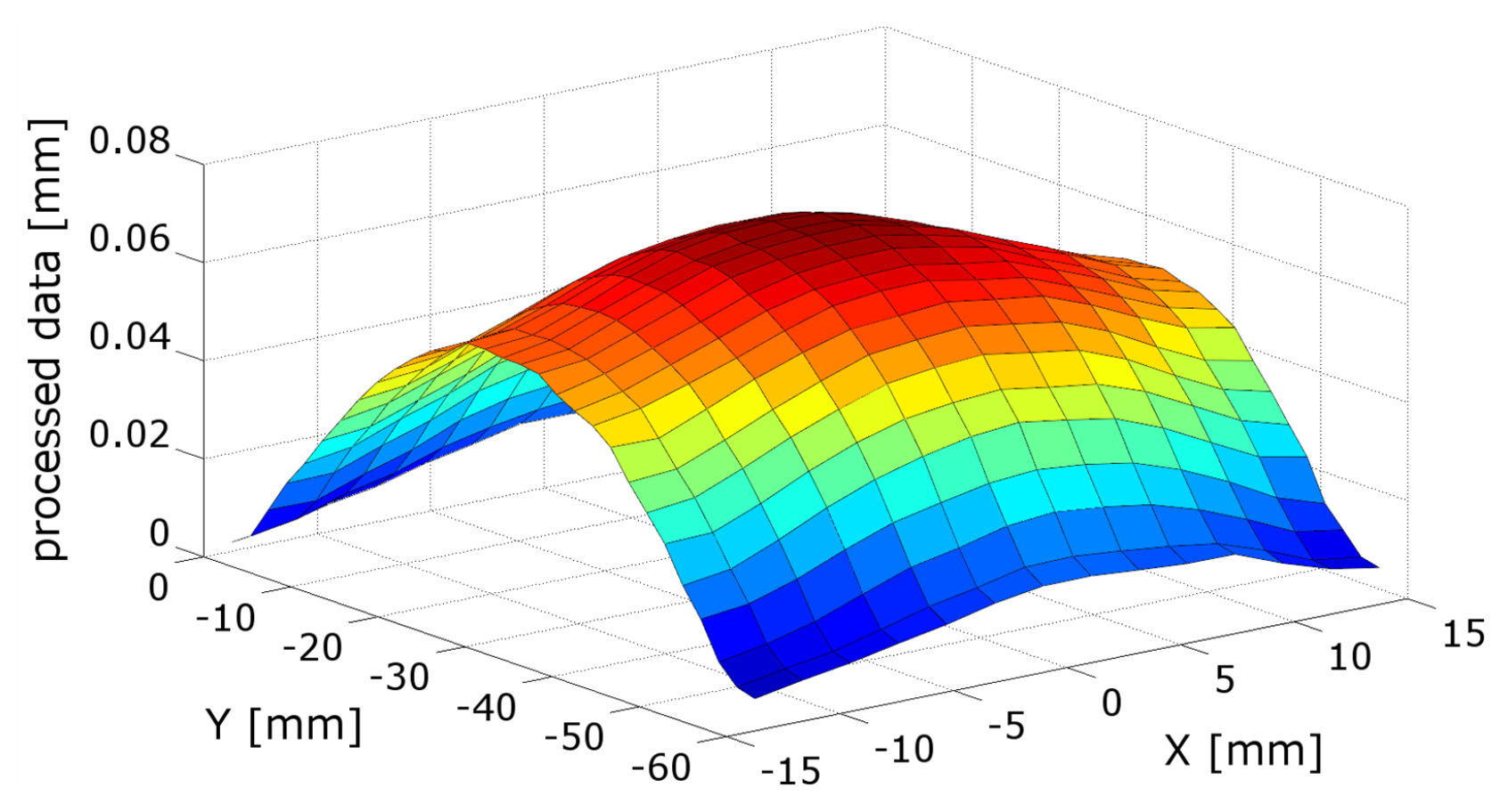
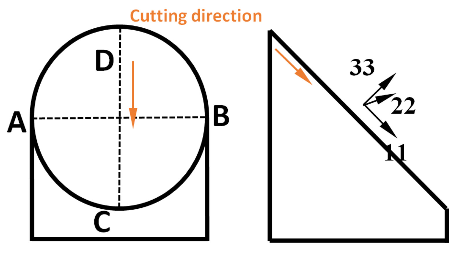
2.7. FE Simulation of the Contour Cut Method

The inherent feature of the contour method is that it provides information on stresses perpendicular to the cut plane. The discussion below deals with the other components of the stress tensor, including the in-plane stresses on the cut plane which by definition are not considered by the contour method. Determination of all stress components after cutting was studied in [17,18]. However, the methods are rather complicated.

Our approach is based on evaluating a cut surface which deforms freely in all directions during cutting. Measurement in normal direction to the surface and subsequent smoothing preserves this information. The same approach was used to determine residual stresses in quenching of aluminum forged part [19], but no prove of used approach was given.

We also studied the discrepancies between the stress components determined by the contour method and by the FE analysis of heat treatment. The coordinate system was chosen so as to ensure that identical stress components were compared.

An FE simulation of the contour cut method was performed in two steps. The first step was the FE simulation of the heat treatment. Its results shown as the stress on a symmetry plane are in Figure 18, Figure 19 and Figure 20. The stress directions 11, 22 mean tangential stresses and 33 direction mean normal stress to the cut plane.

Then, the symmetry condition was removed and the resulting displacement normal to the symmetry plane is relevant to the displacement measured after cutting. In the second step, this displacement was reversed and imposed on the symmetry/cut plane to simulate the FE analysis conducted as part of the contour method. The results are fully comparable with the heat treatment simulation. Therefore, both normal and tangential stresses can be compared, instead of just the normal stress on the cut surface, as seen in Figure 21, Figure 22 and Figure 23.

Based on this study, we conclude that the whole tensor can be derived using the contour method.

3. Results and Discussion

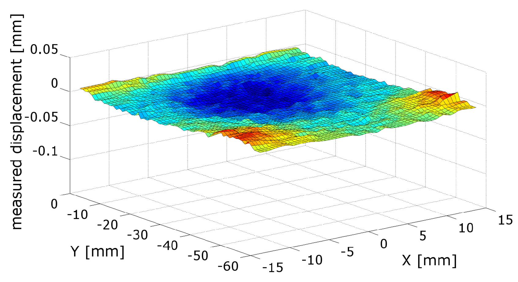
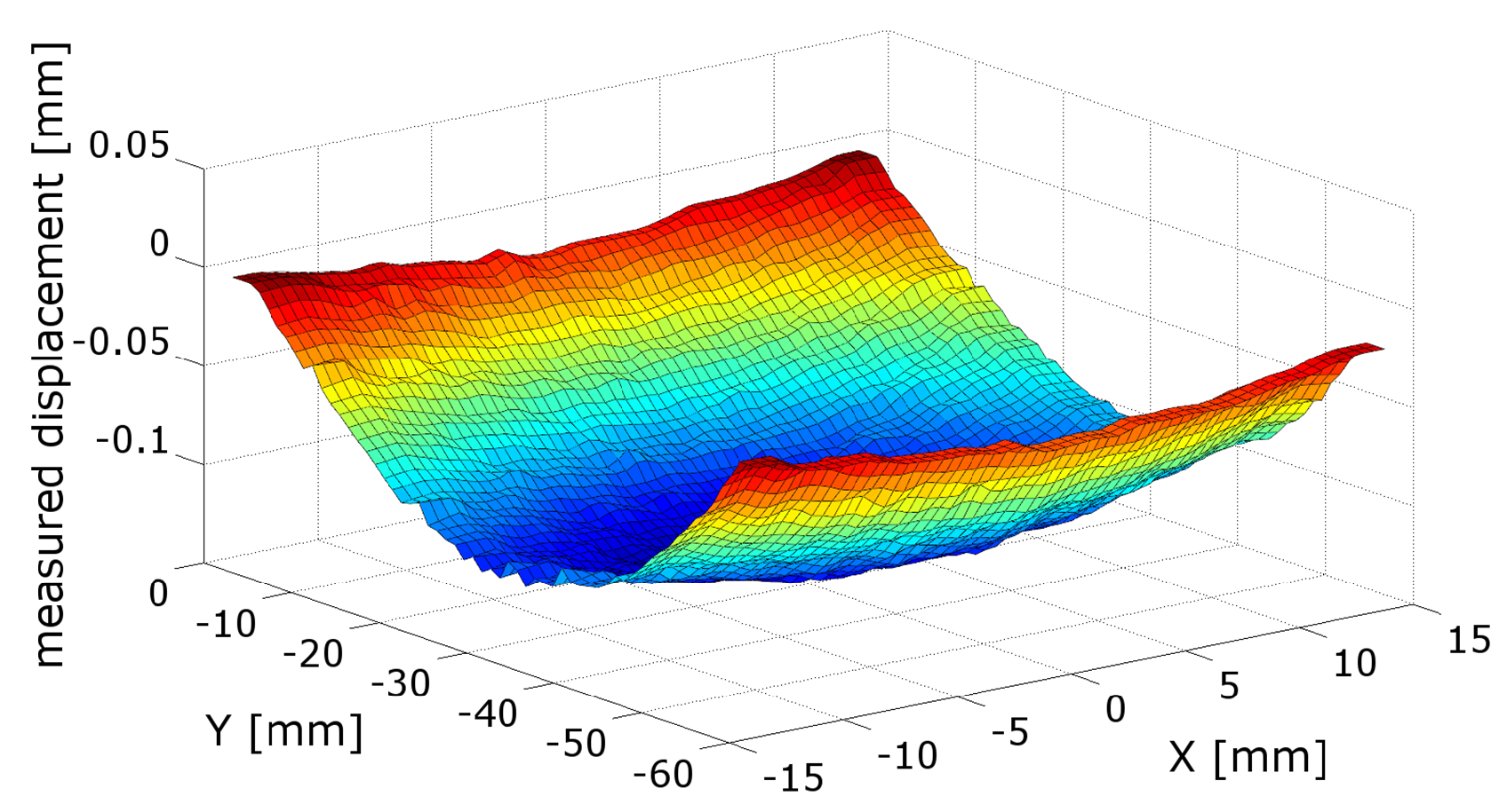
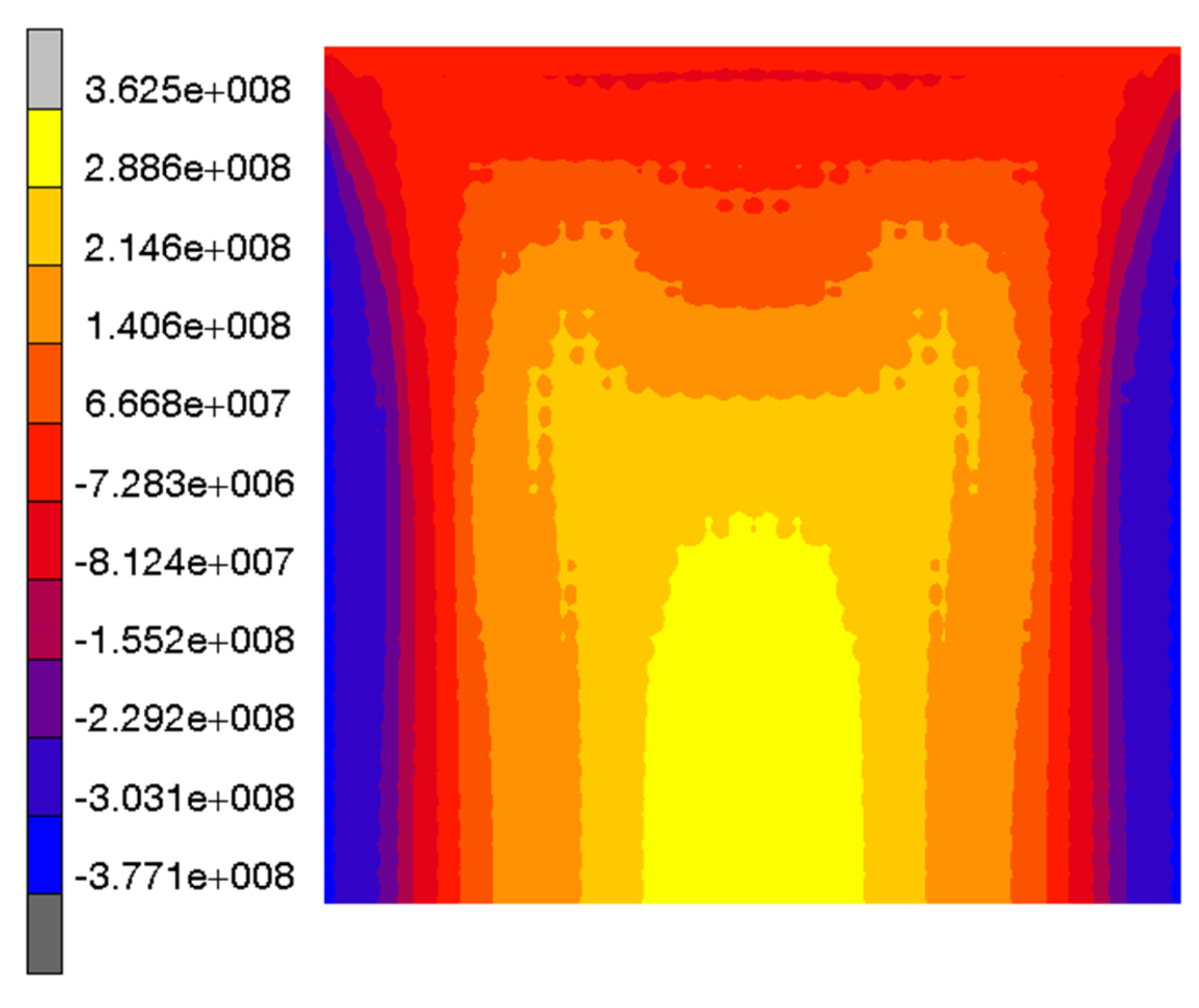
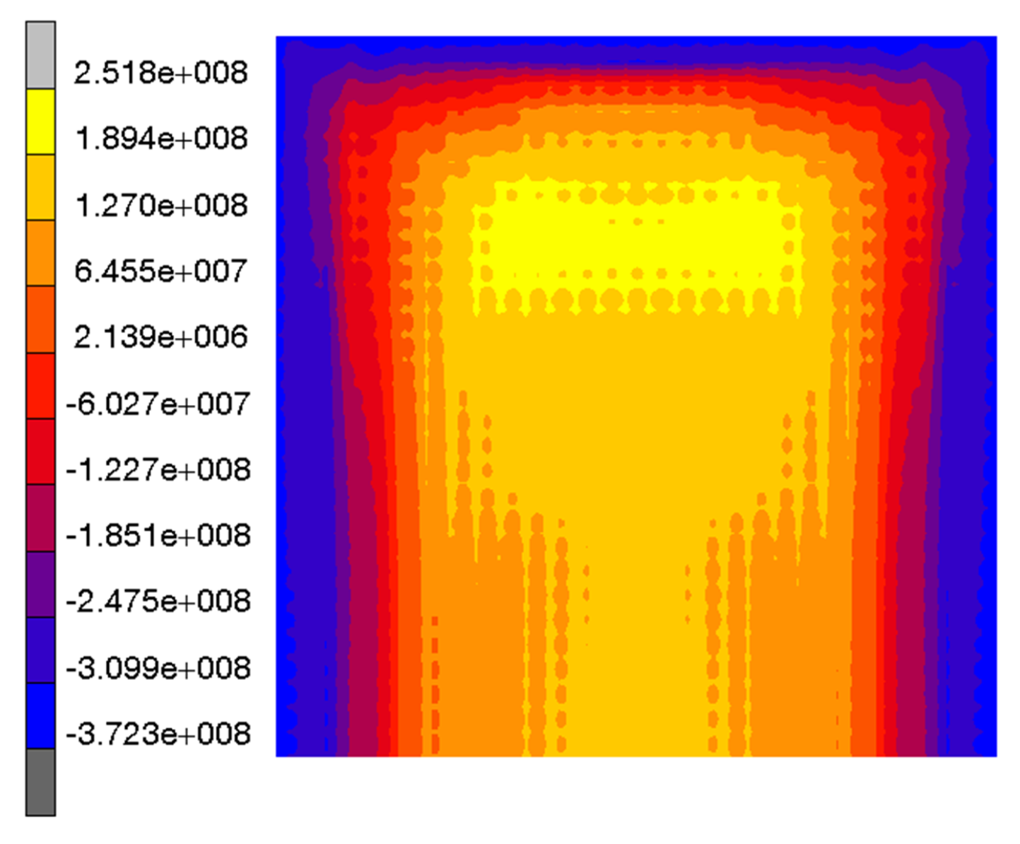
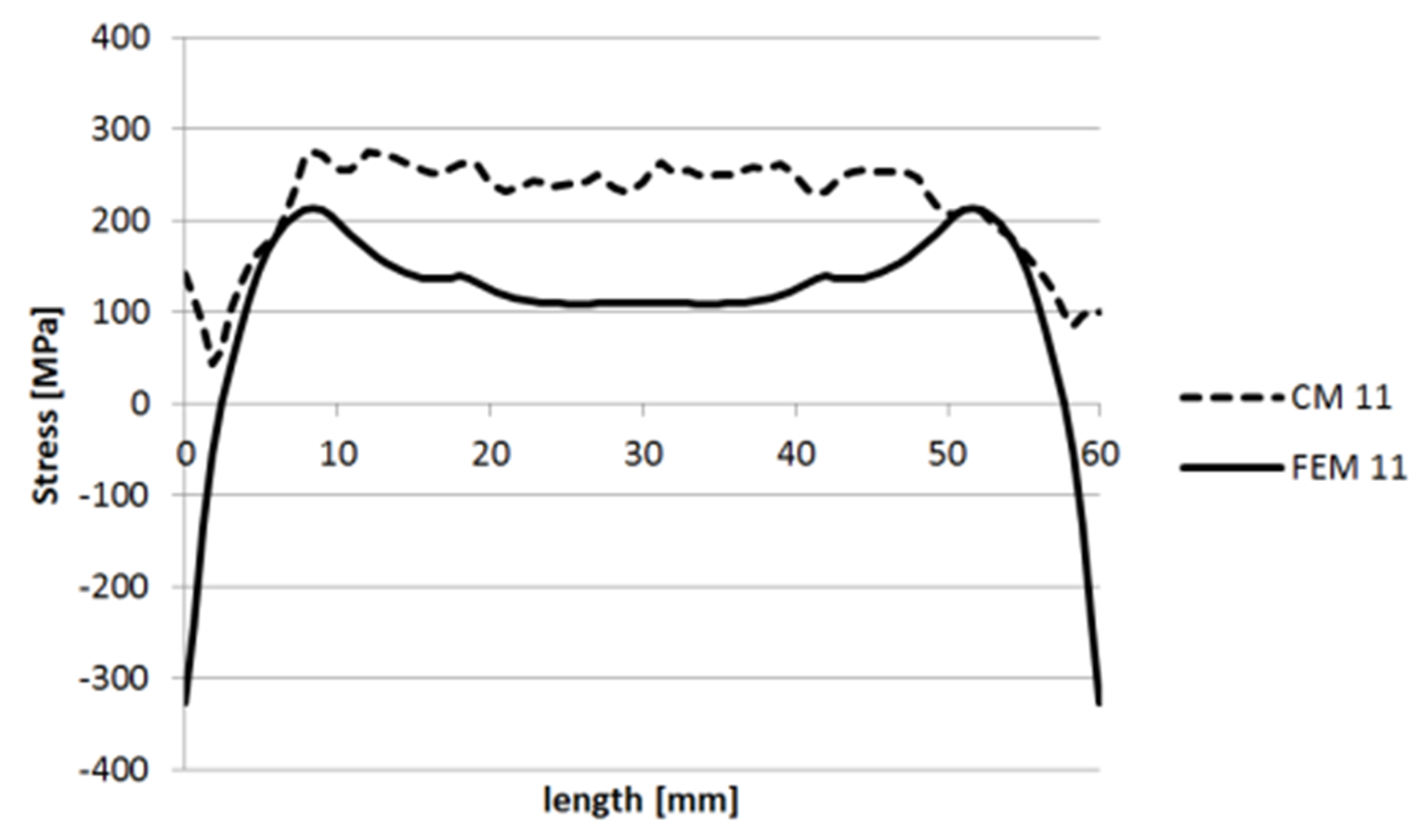
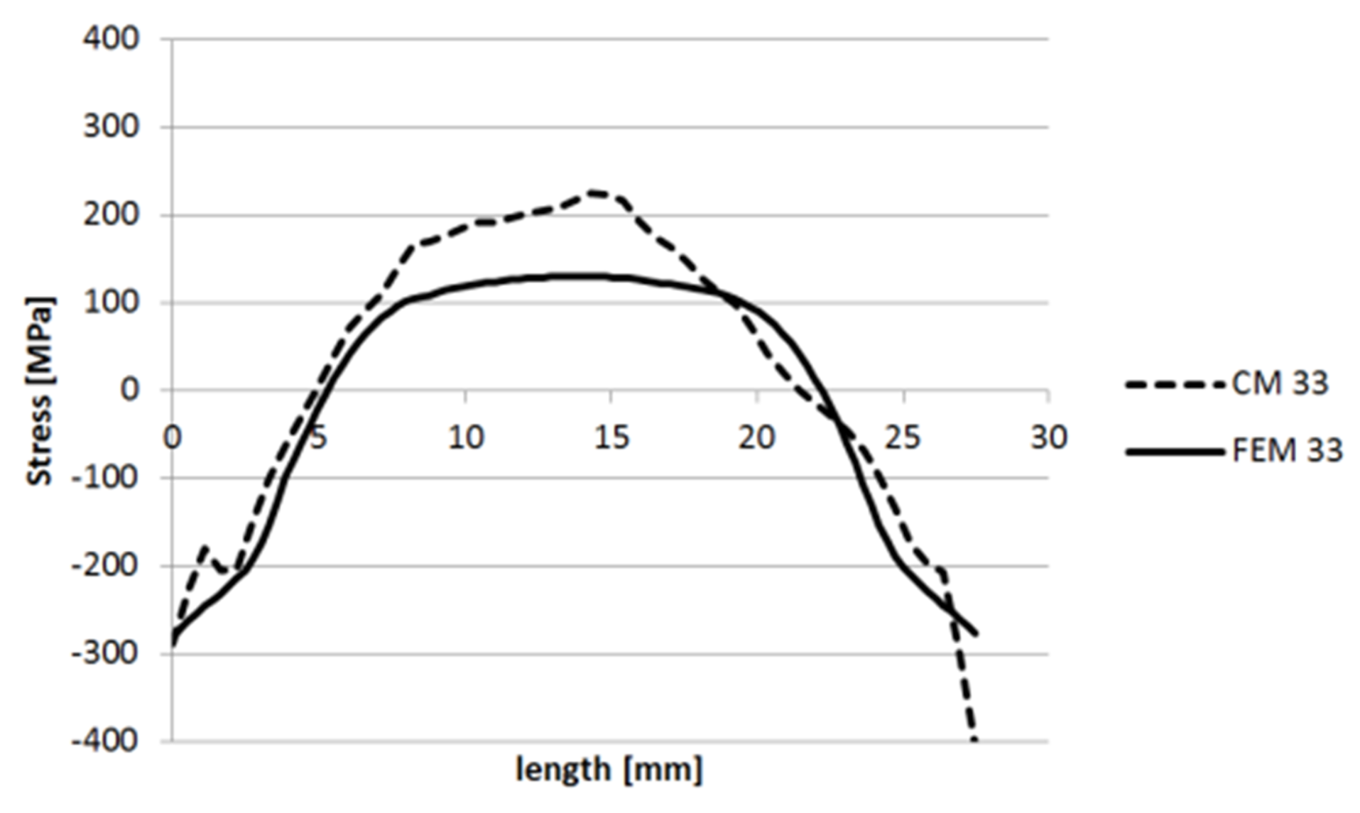
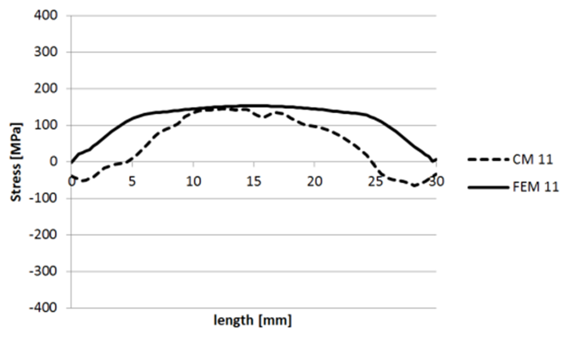
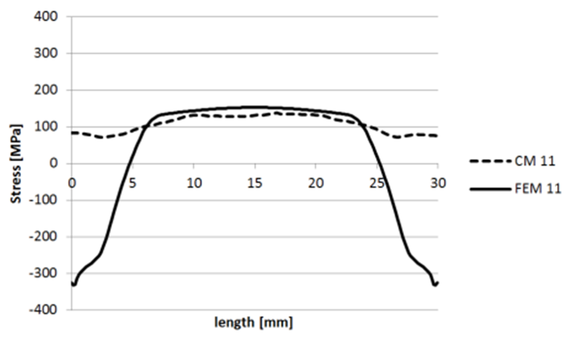
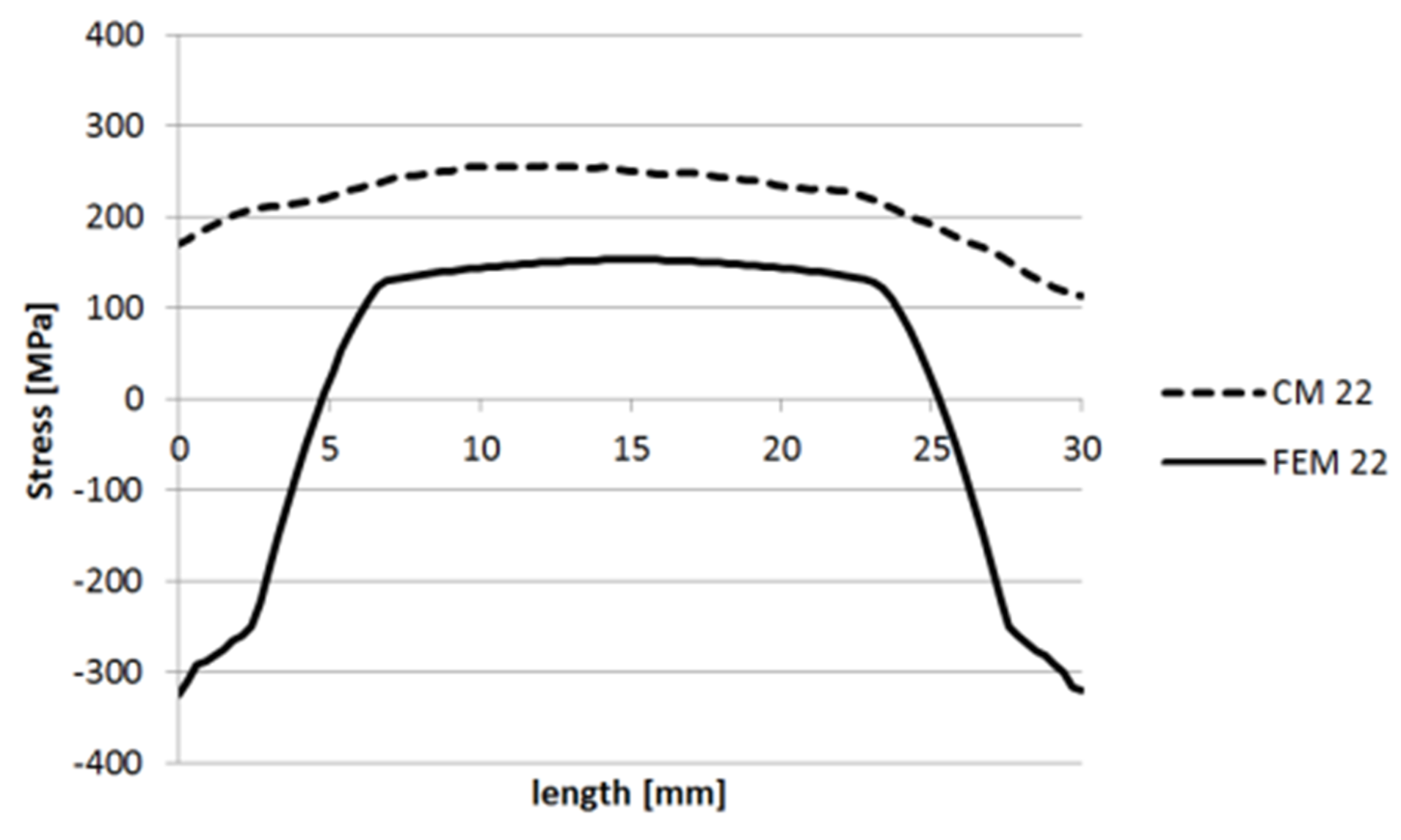
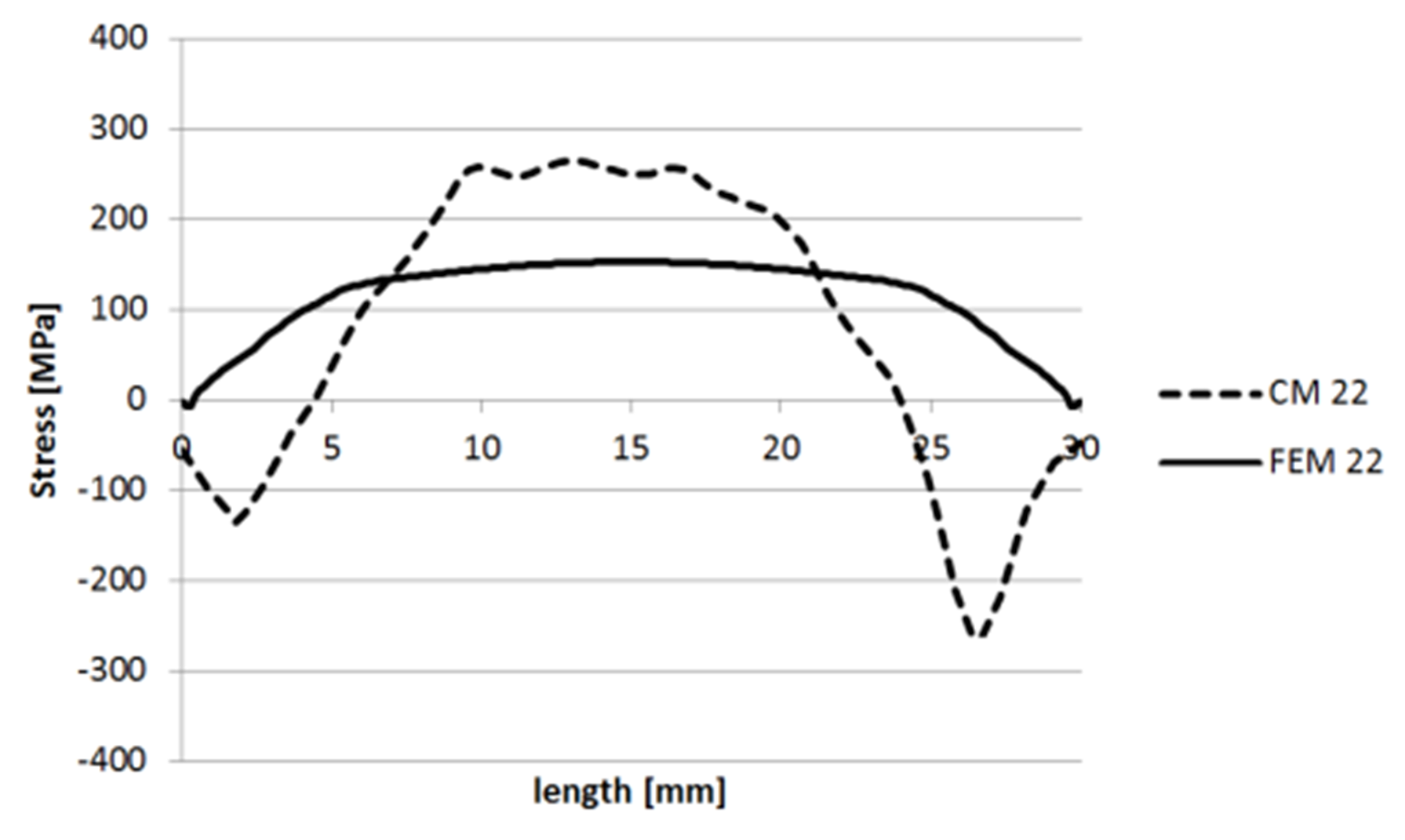
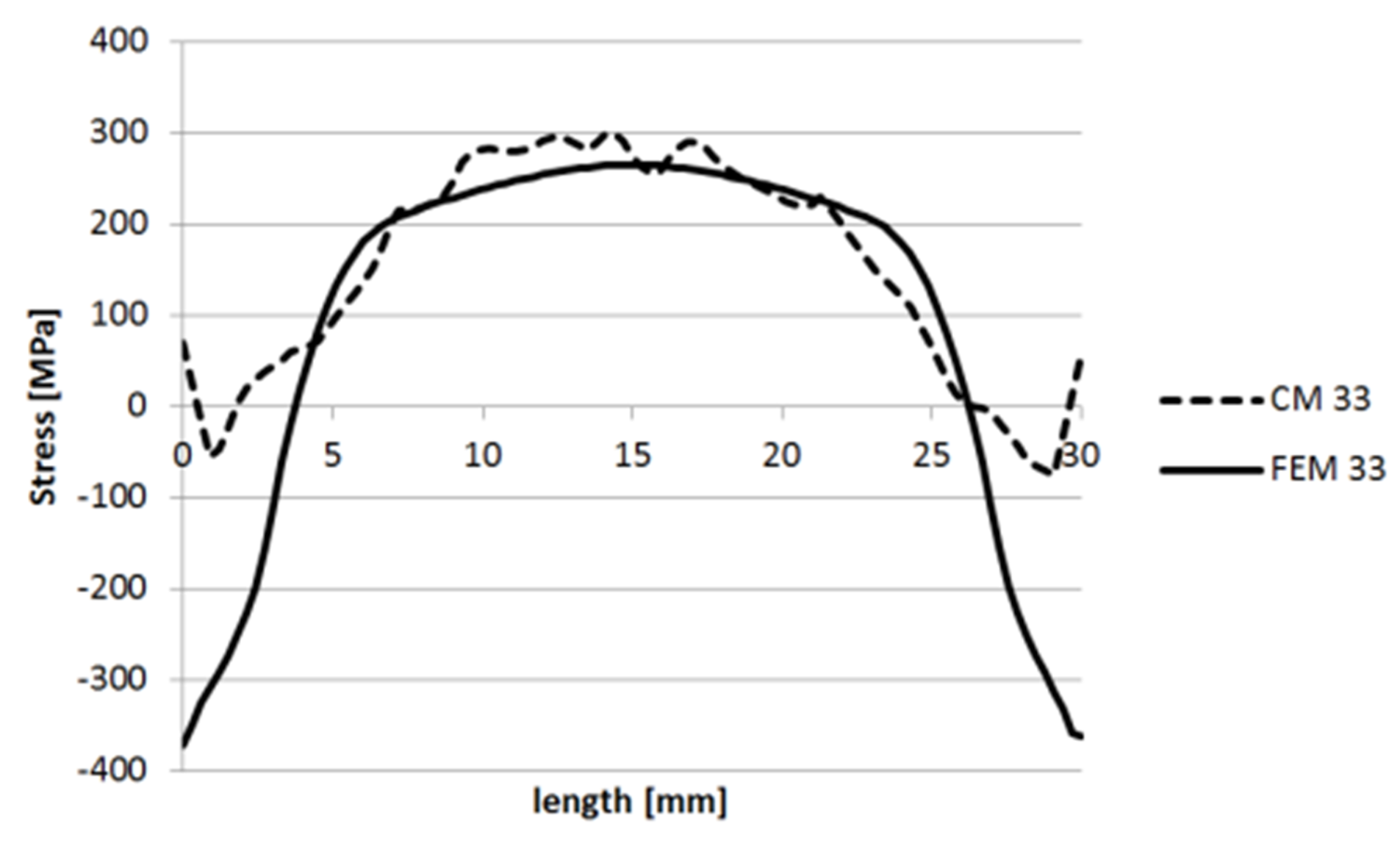
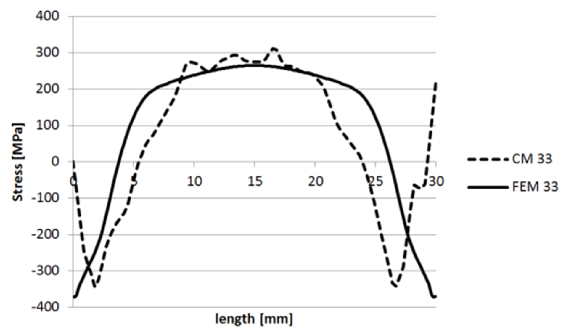
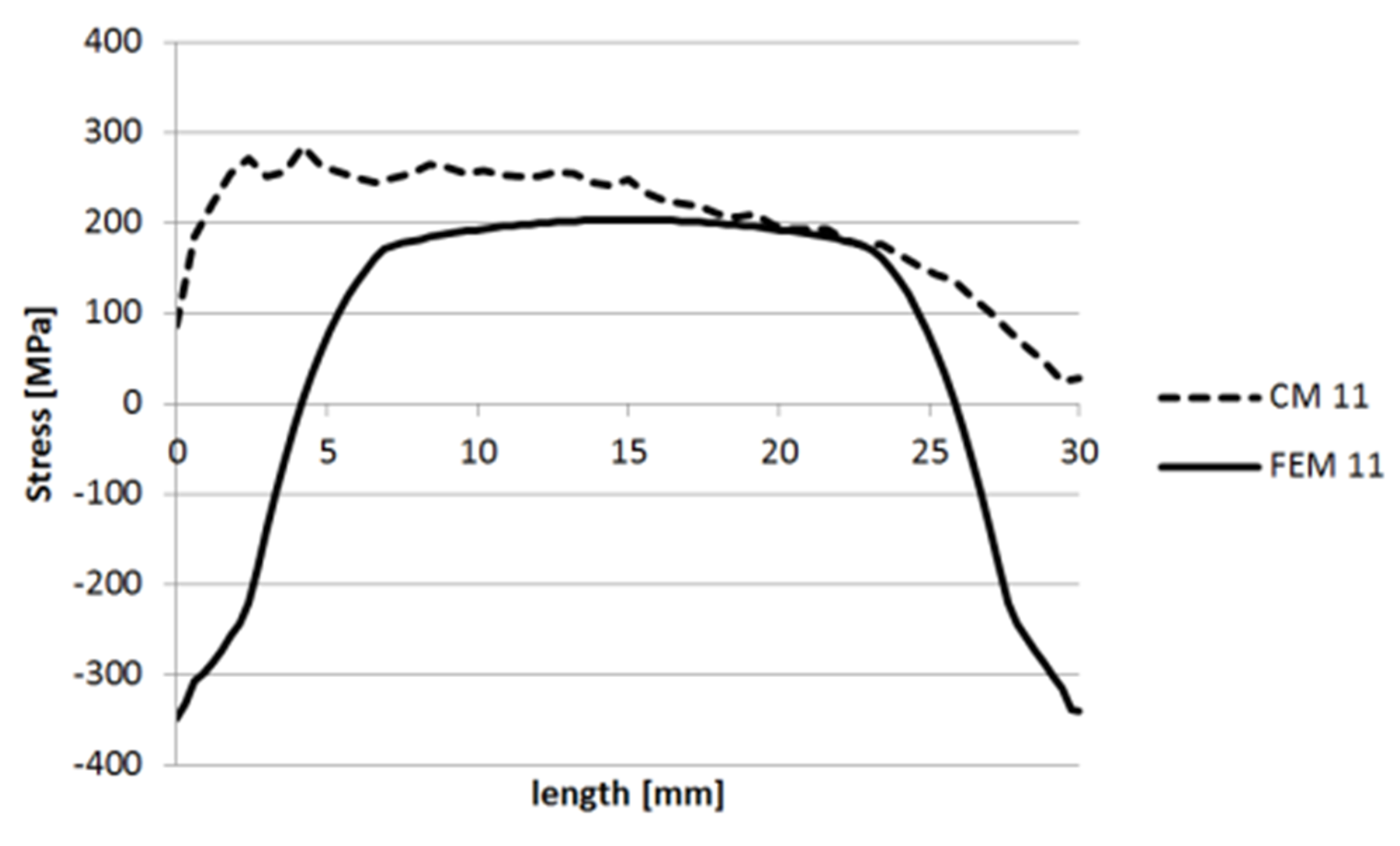
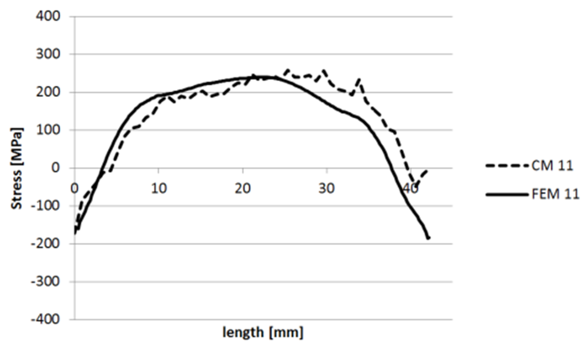
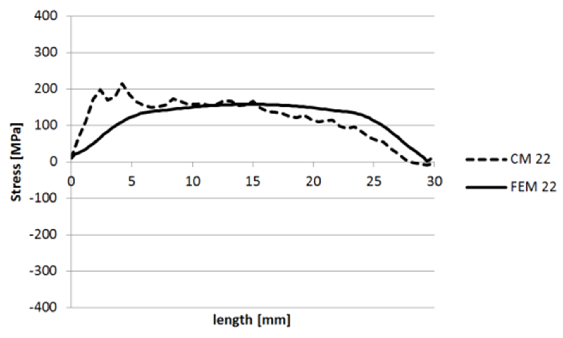
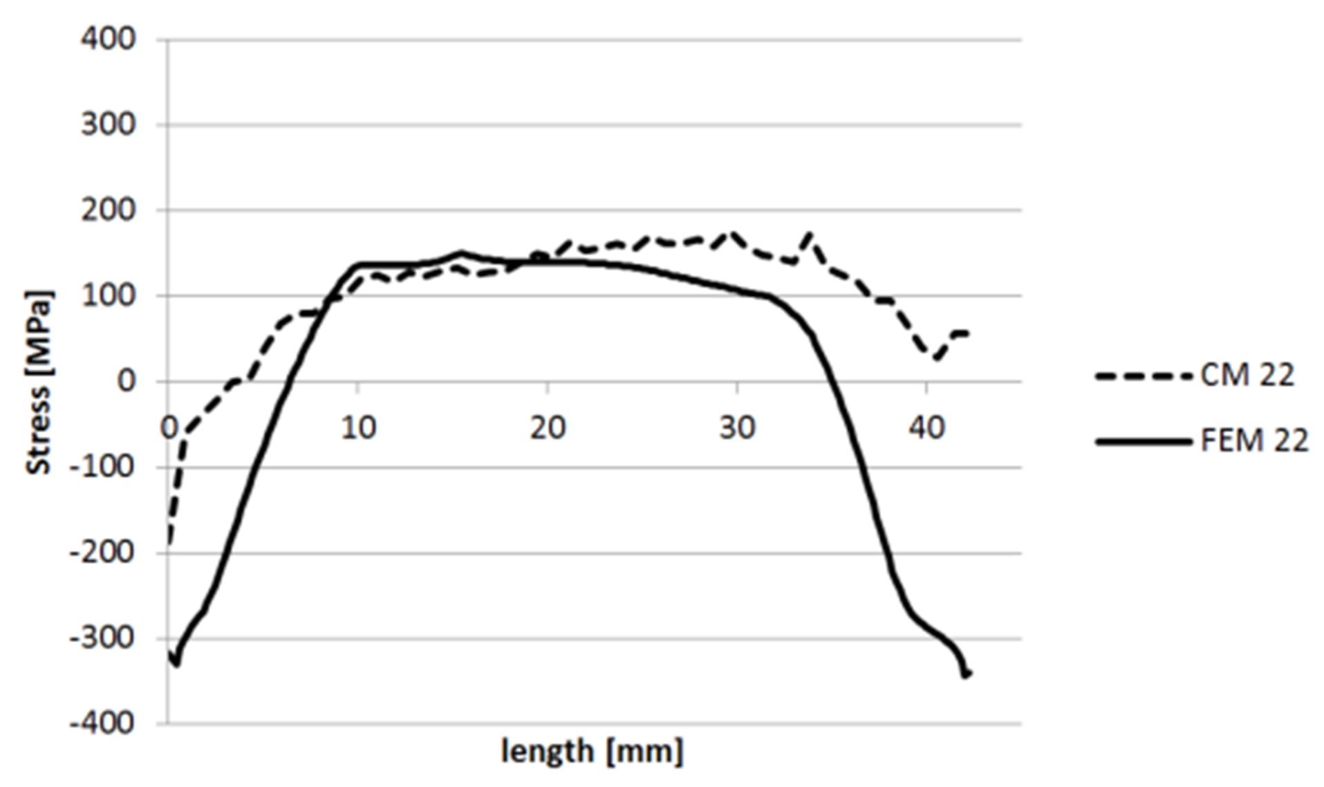
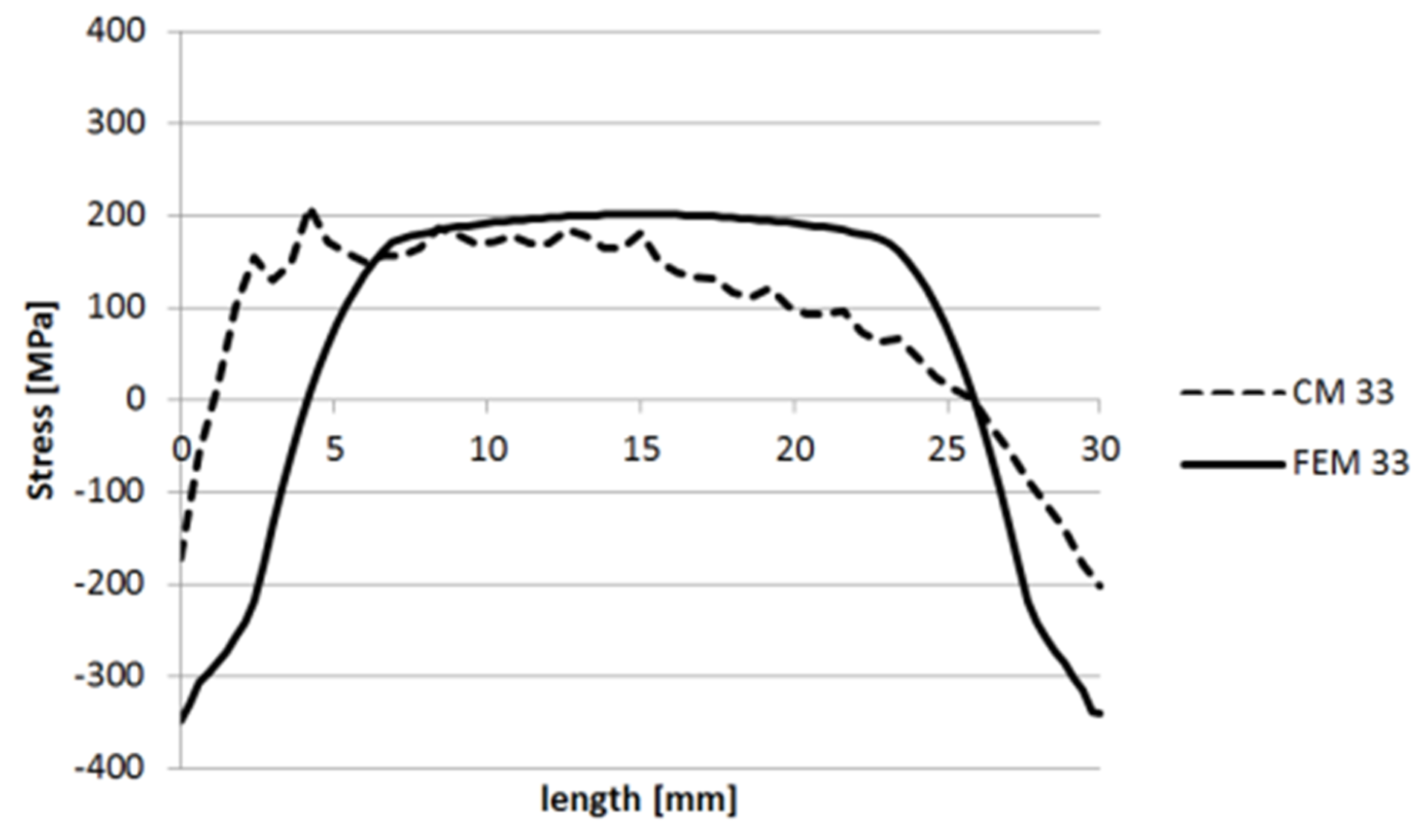
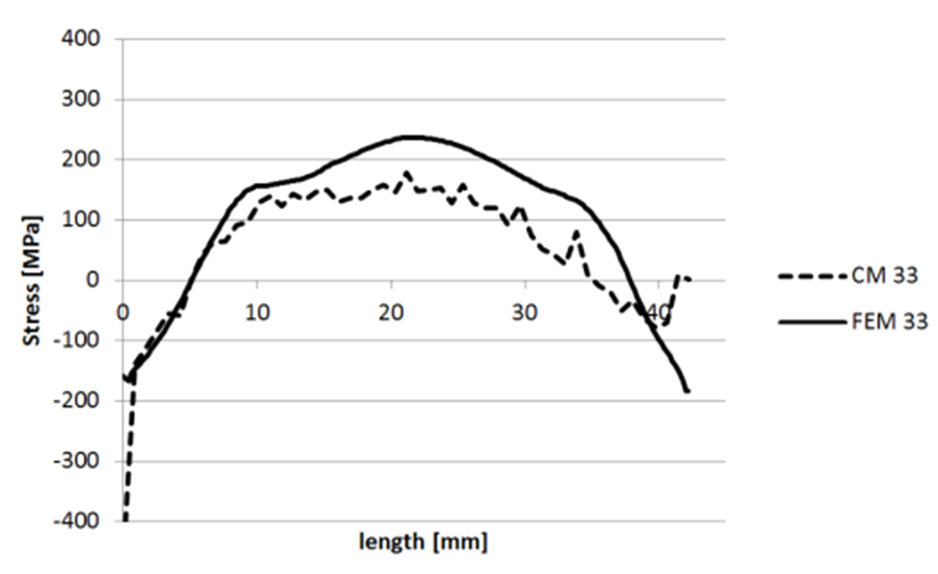
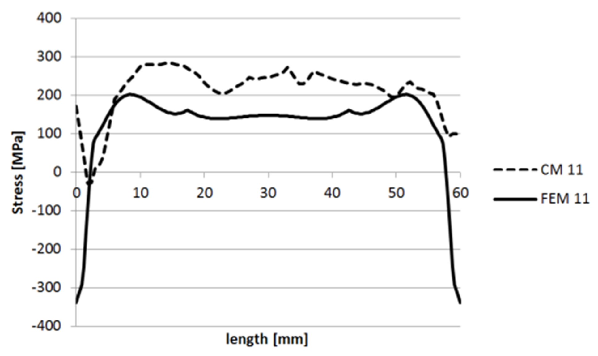
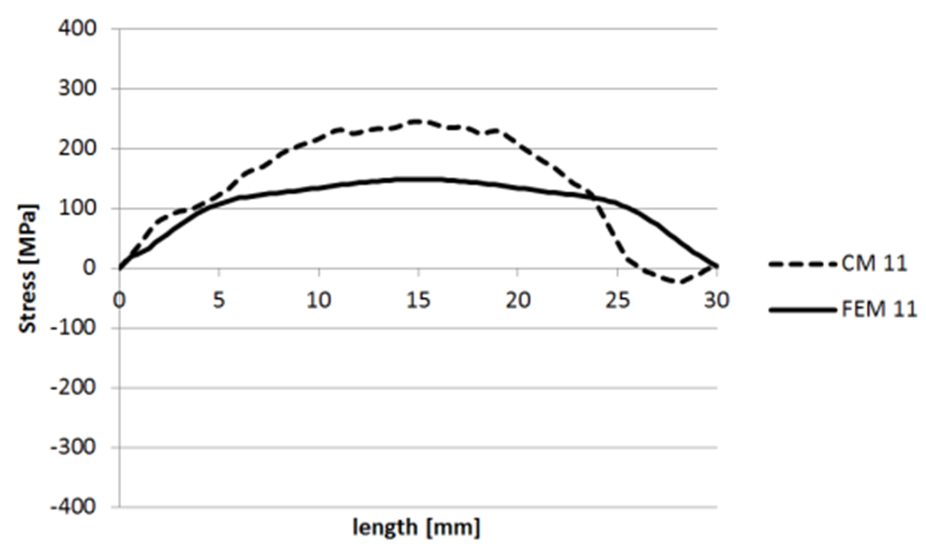
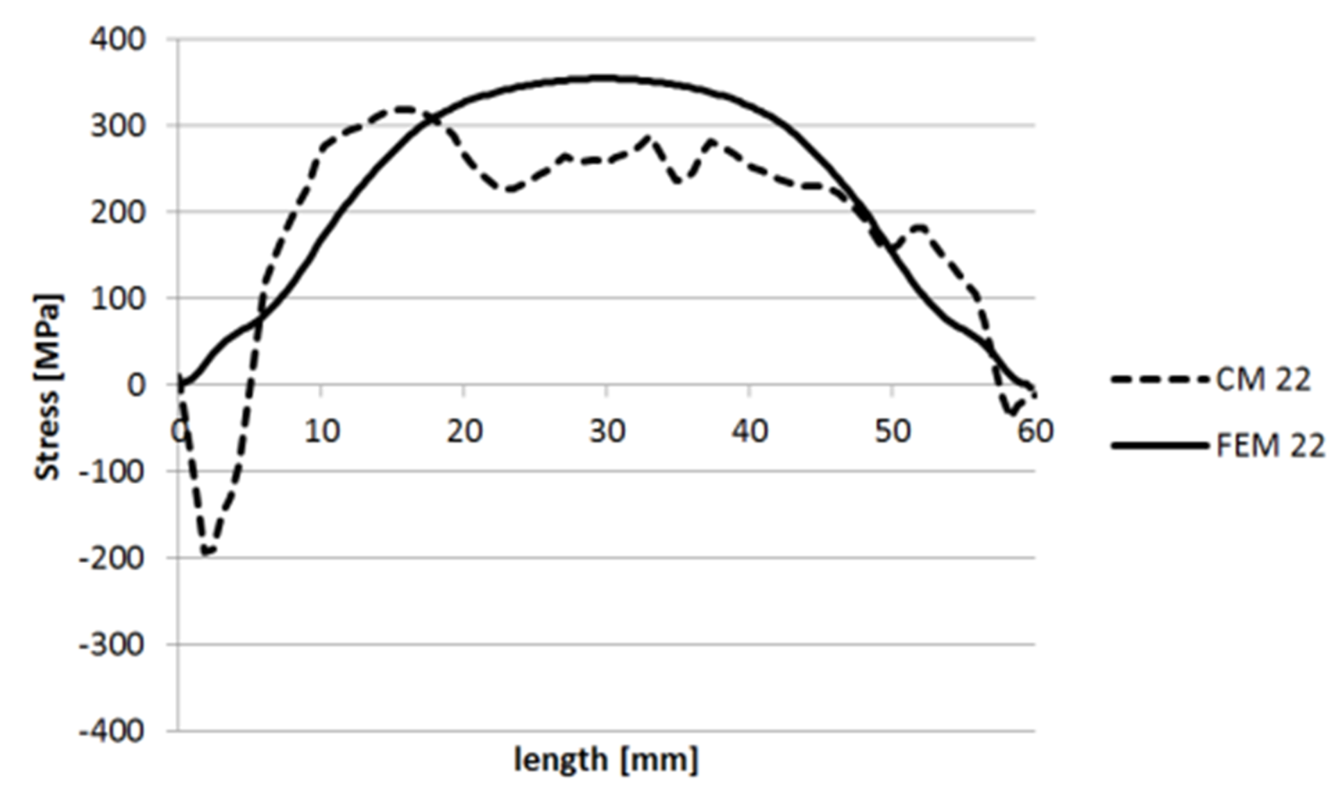
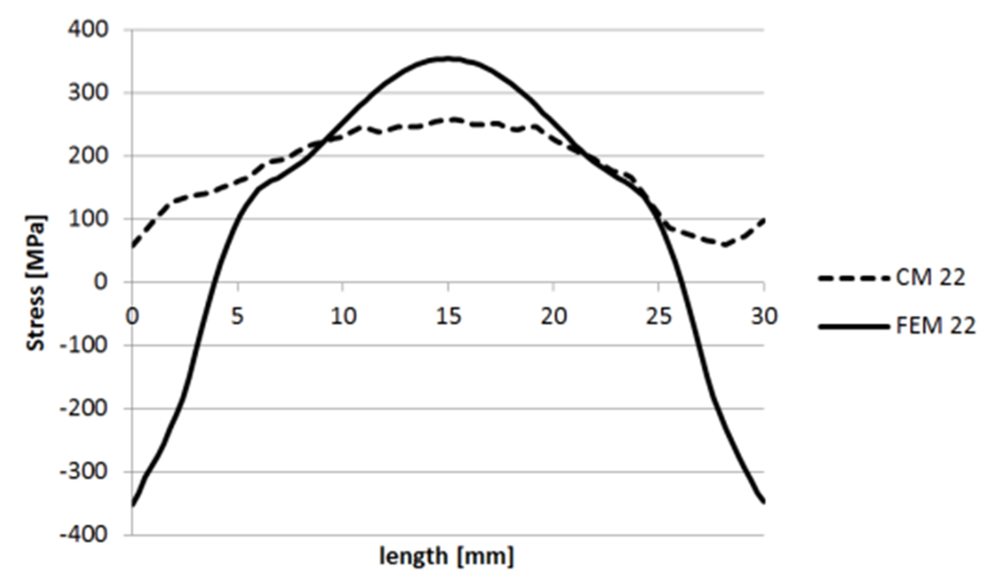
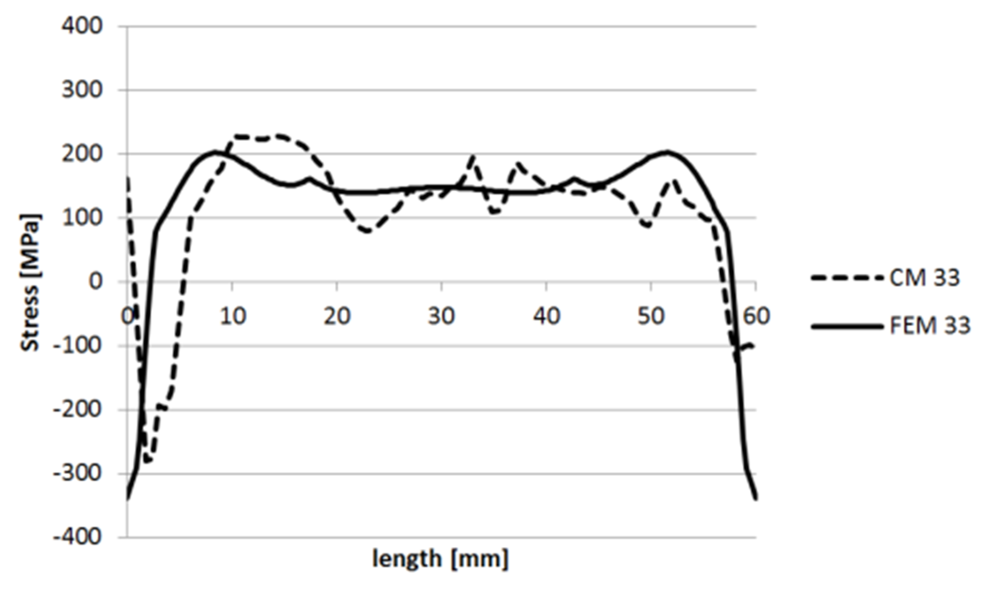
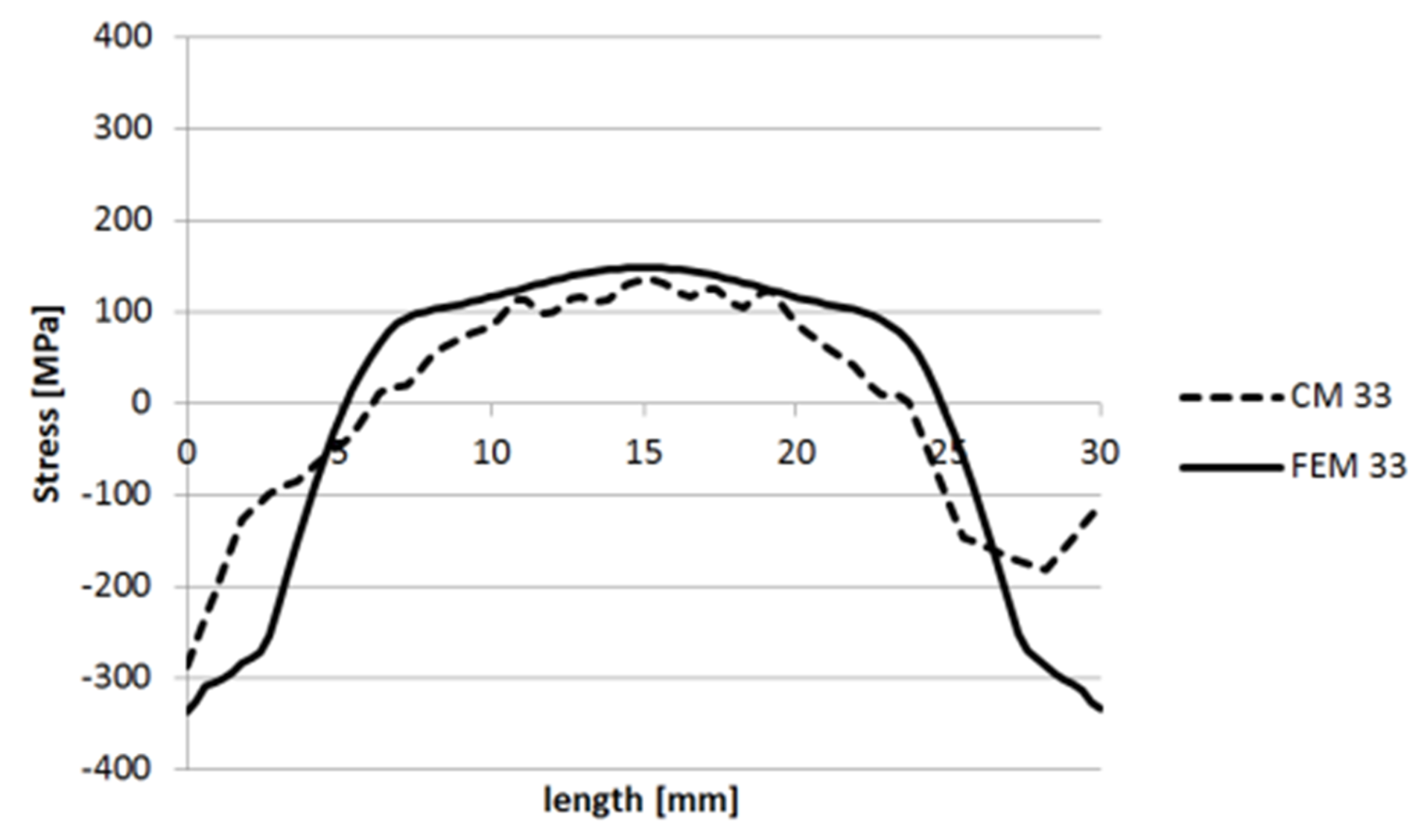
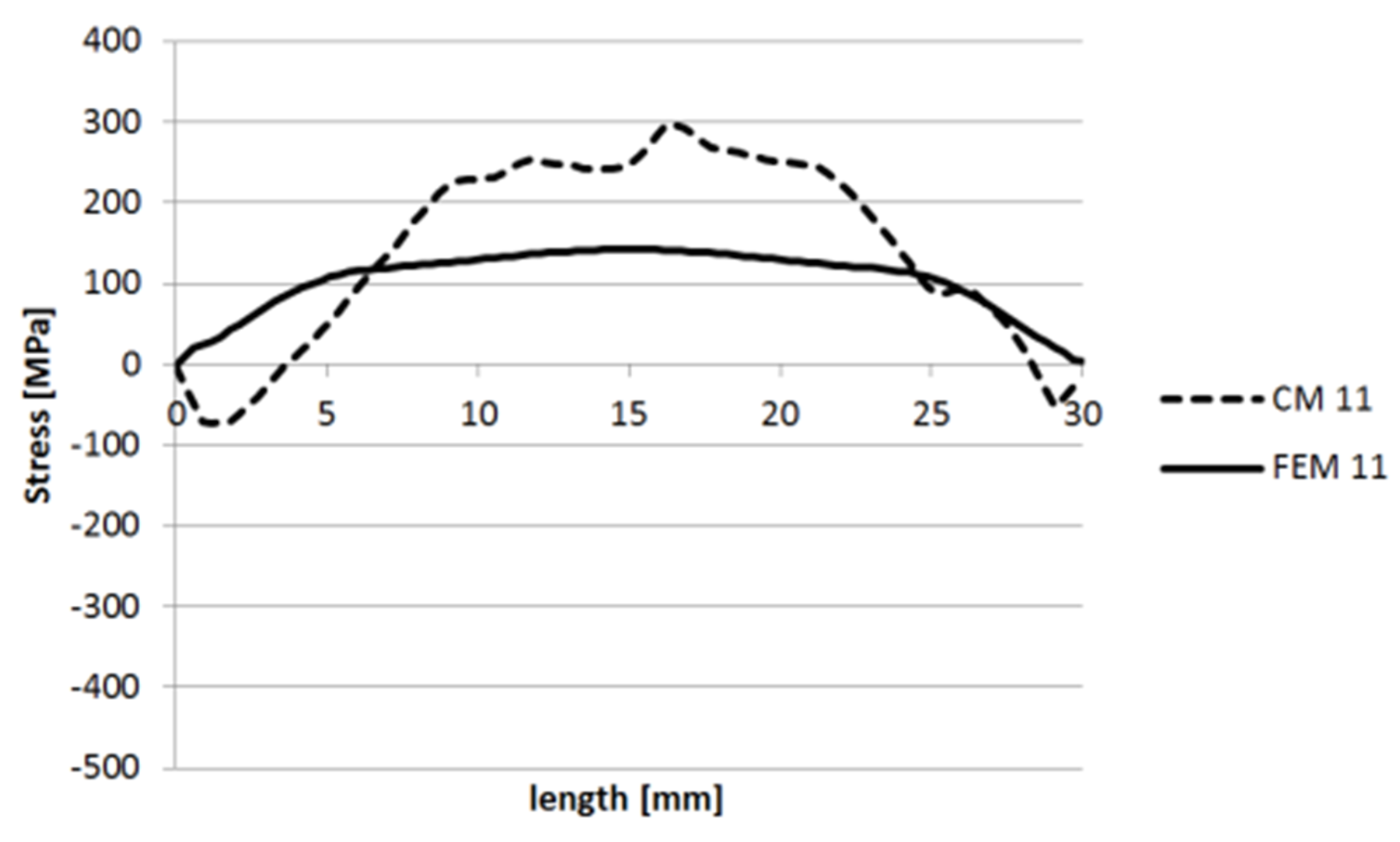
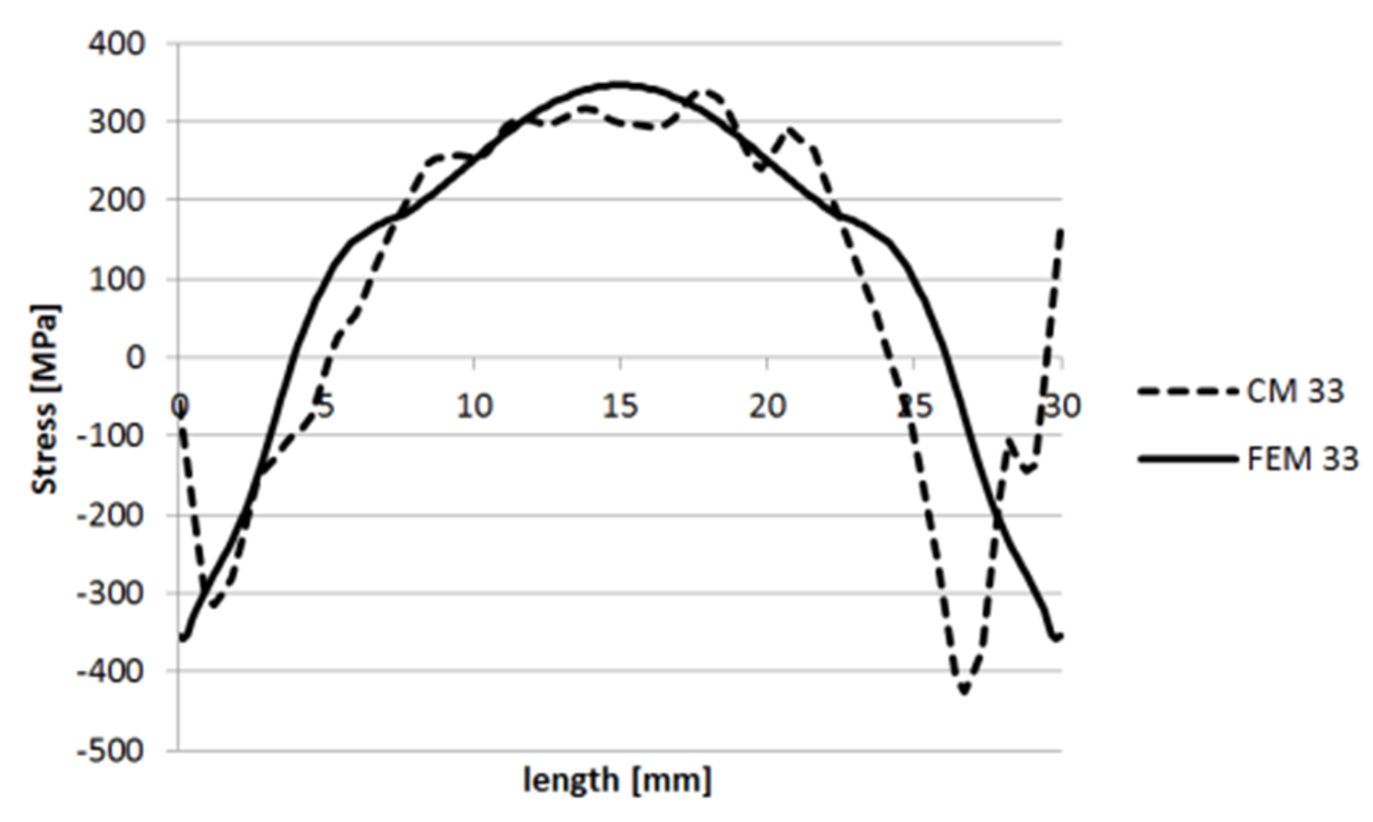
3.1. Comparison of Residual Stresses Determined Using the Contour Method (CM) and Residual Stresses Found by FE Analysis of Heat Treatment (FEM)

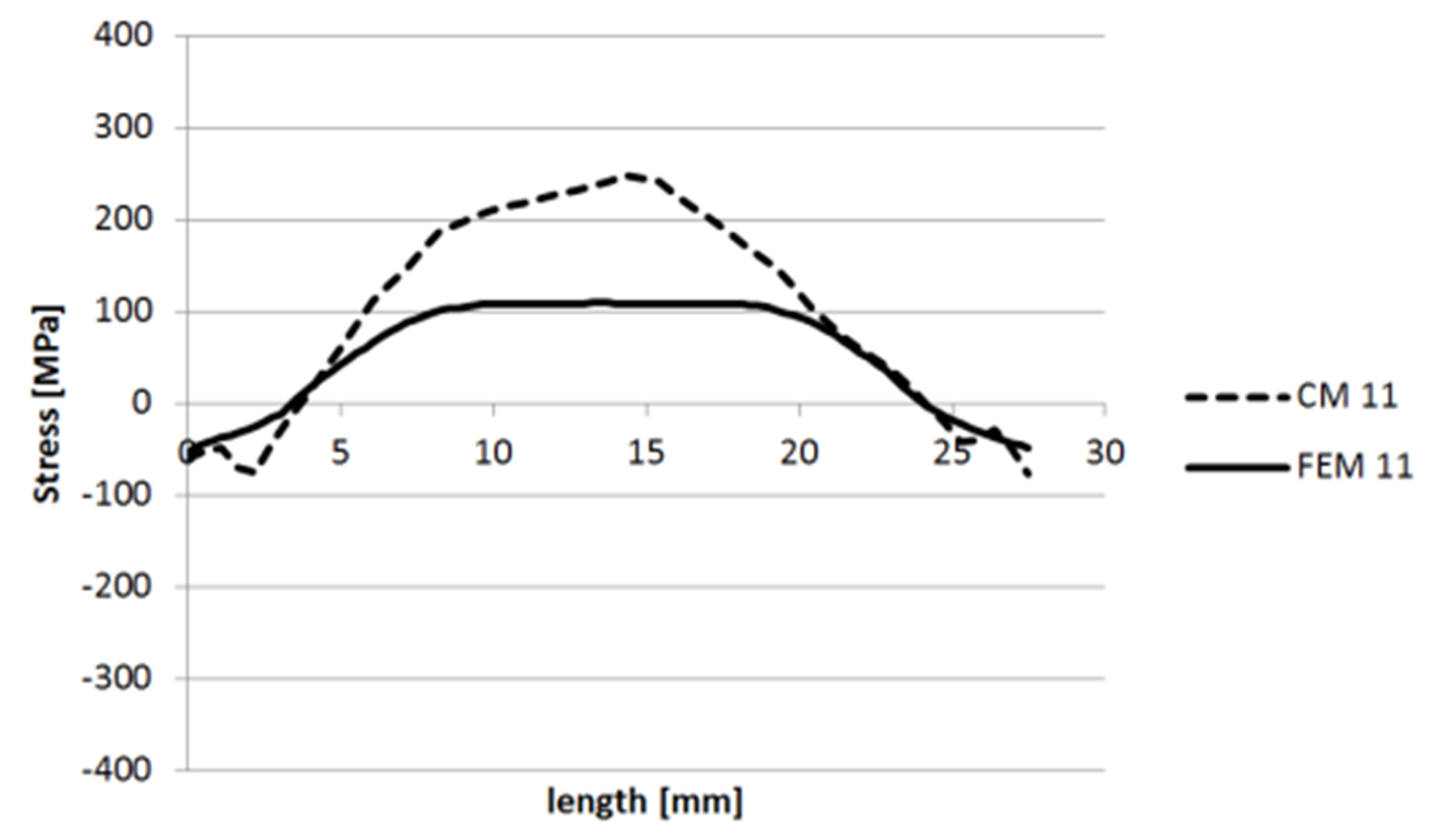
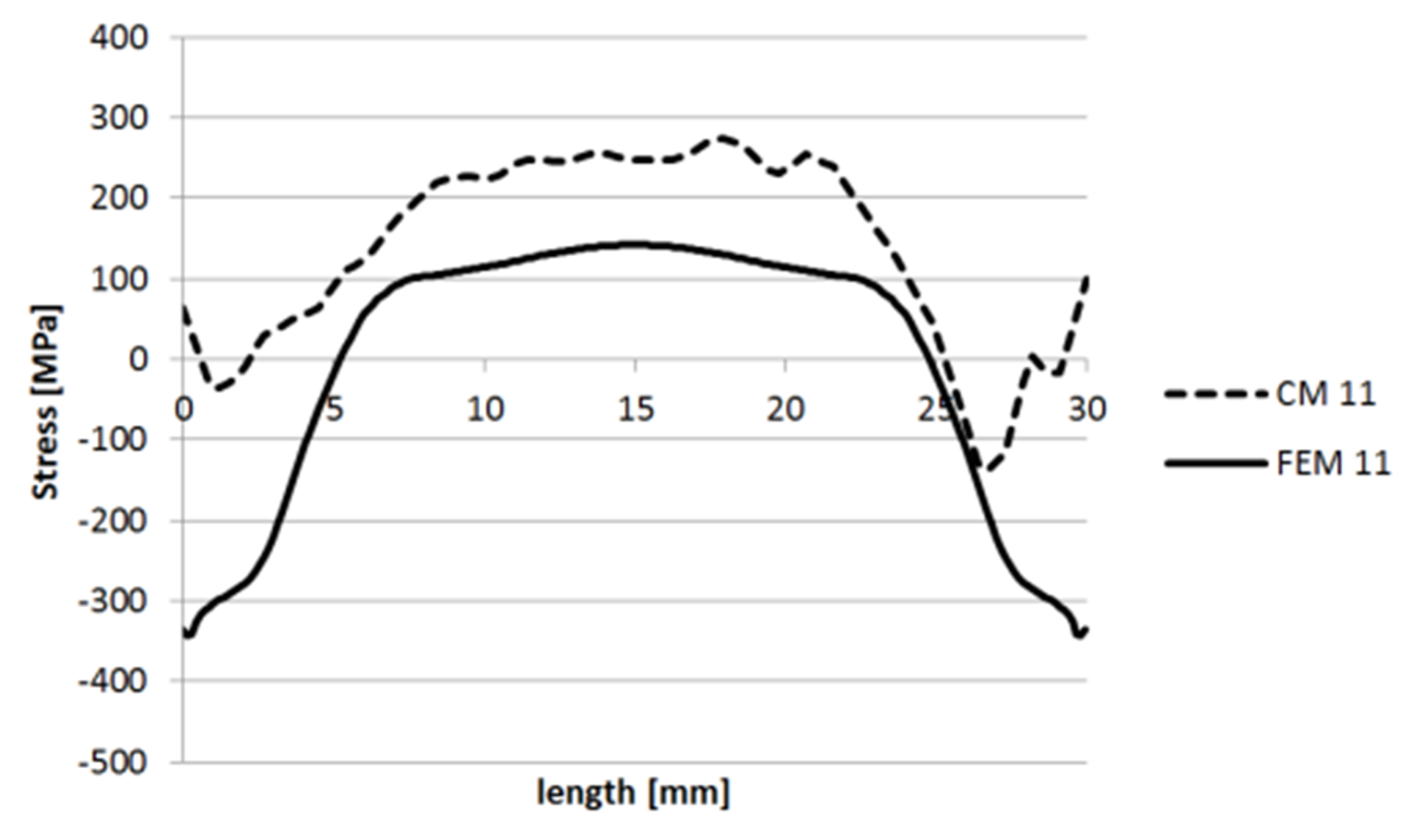
The contour method yields the normal stress distribution along the cut plane (33 direction). Transverse (in-plane) stresses (11 and 22 direction) were computed from the contour method as well and distributions of all the three stresses were compared with residual stresses from the FE model of heat treatment.

3.1.1. Specimen 1

The contour method and FE analysis stresses were compared along line segments AB and CD indicated in Figure 24 along with the system of coordinates. Plots of the contour method and FE stresses for speciment 1 are shown in Figure 25, Figure 26, Figure 27, Figure 28, Figure 29 and Figure 30.

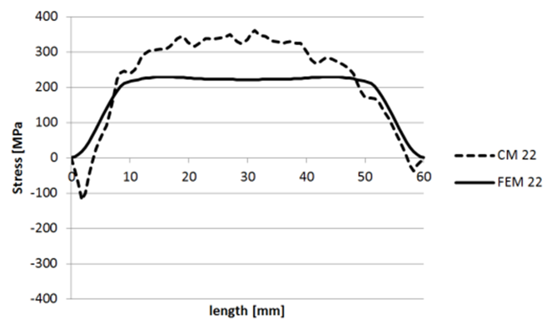
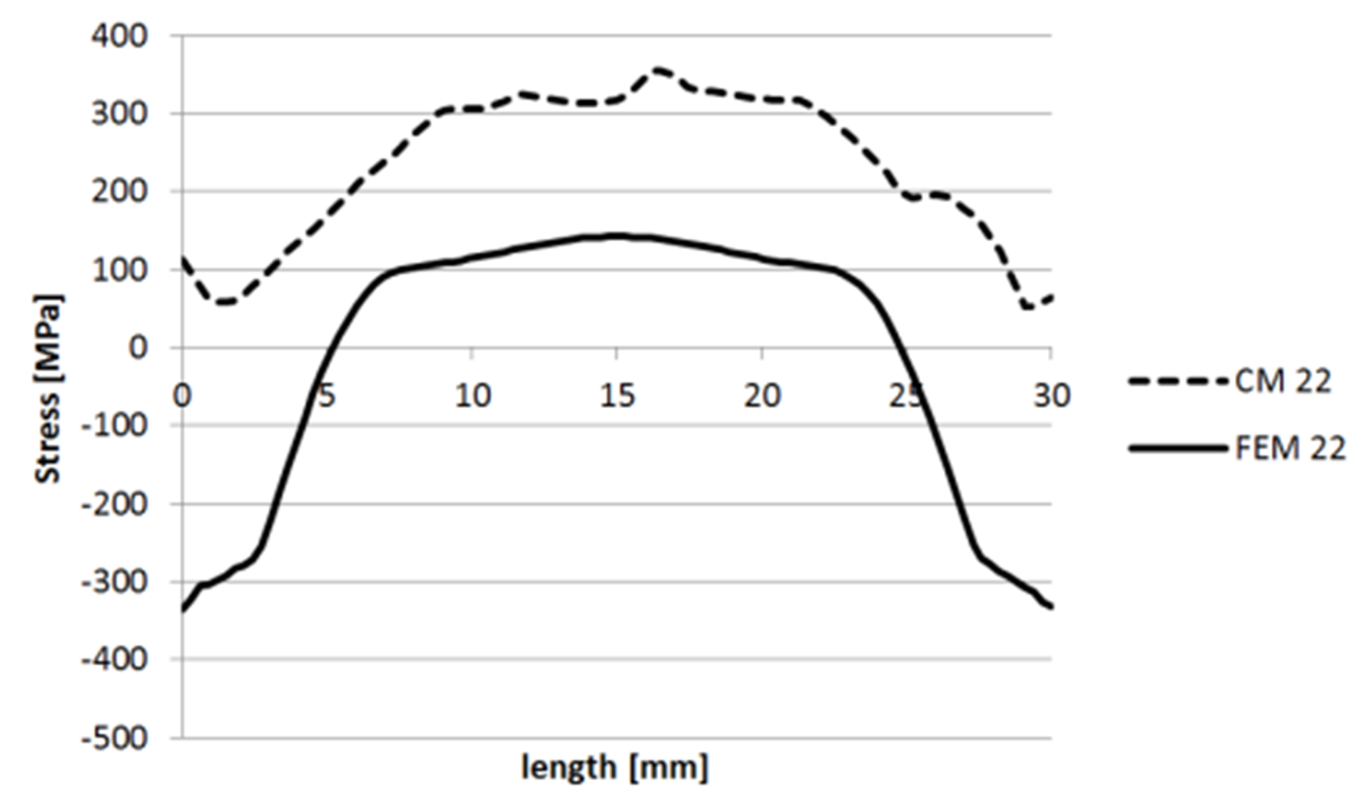
3.1.2. Specimen 2—Cut 1

The contour method and FE analysis data were compared for line segments AB and CD indicated in Figure 31 along with the system of coordinates. Plots of the contour method and FE stresses for speciment 2 - cut 1 are shown in Figure 32, Figure 33, Figure 34, Figure 35, Figure 36 and Figure 37.

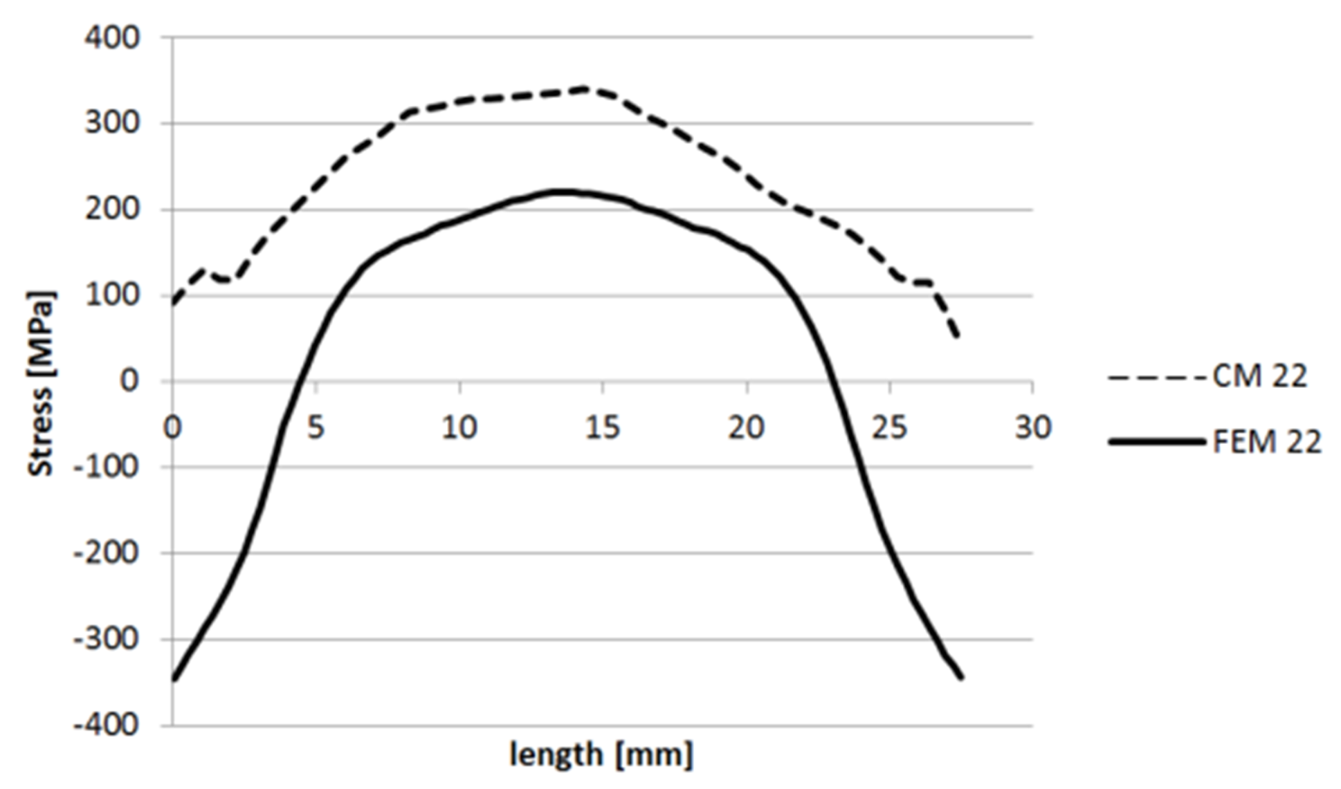
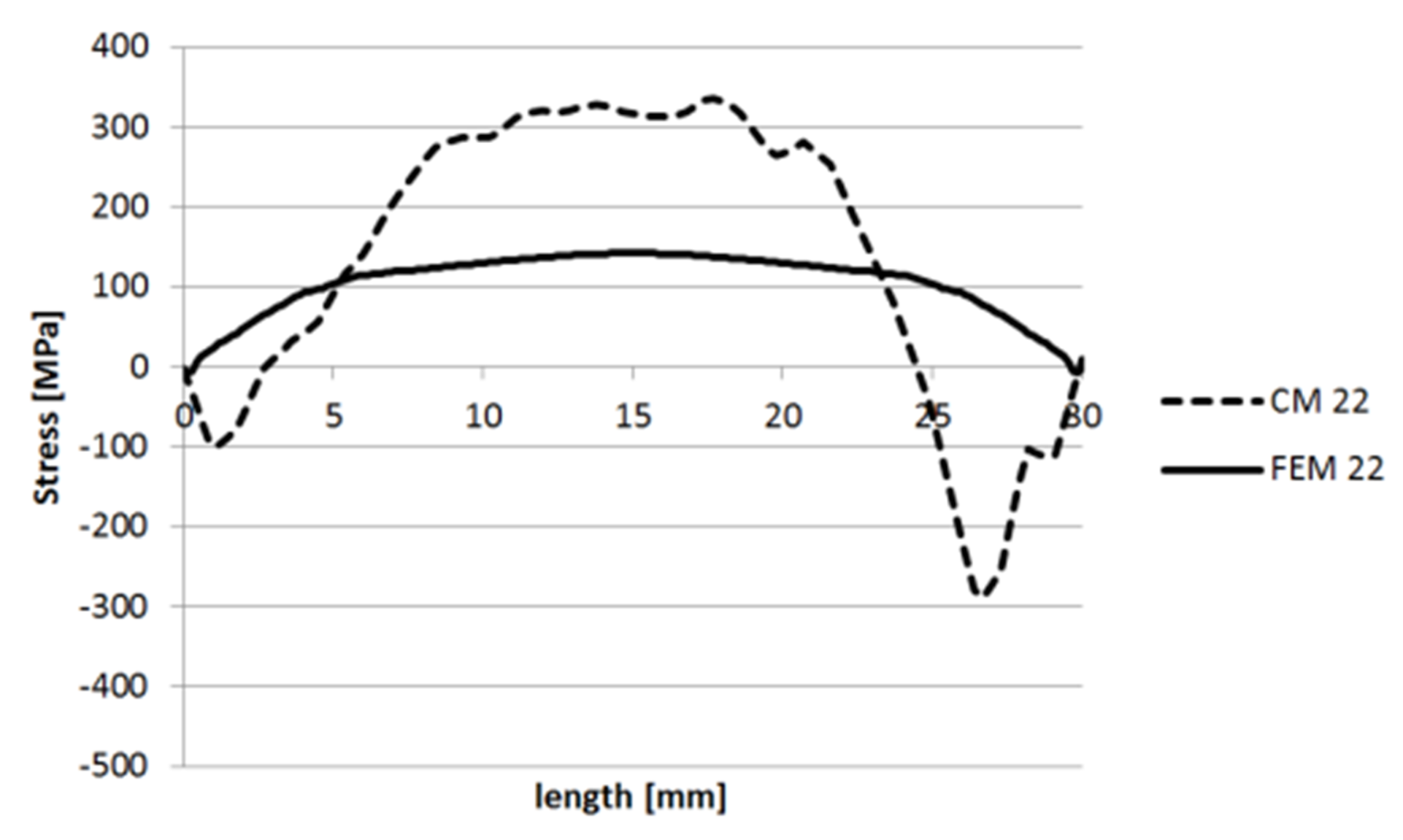
3.1.3. Specimen 2—Cut 2

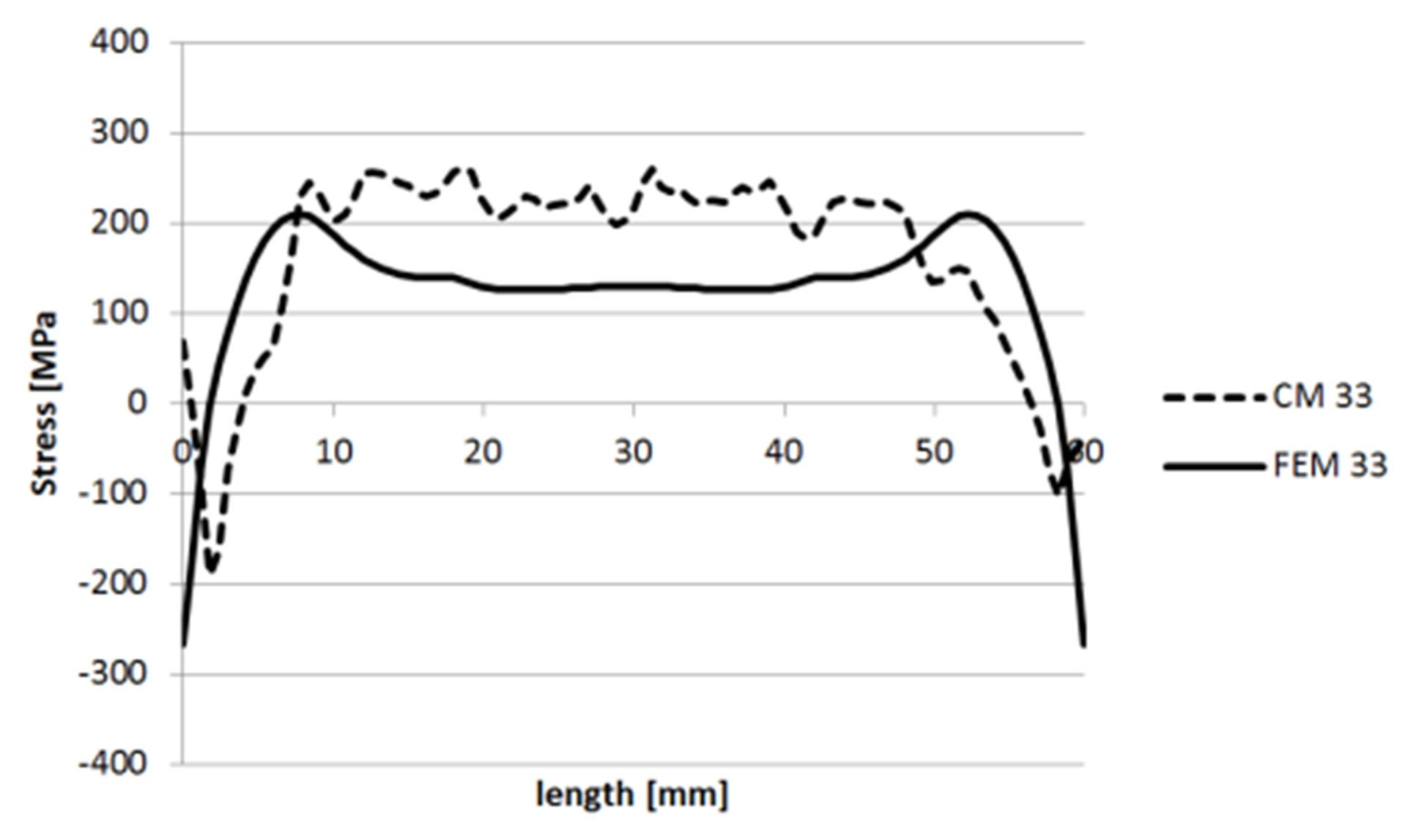
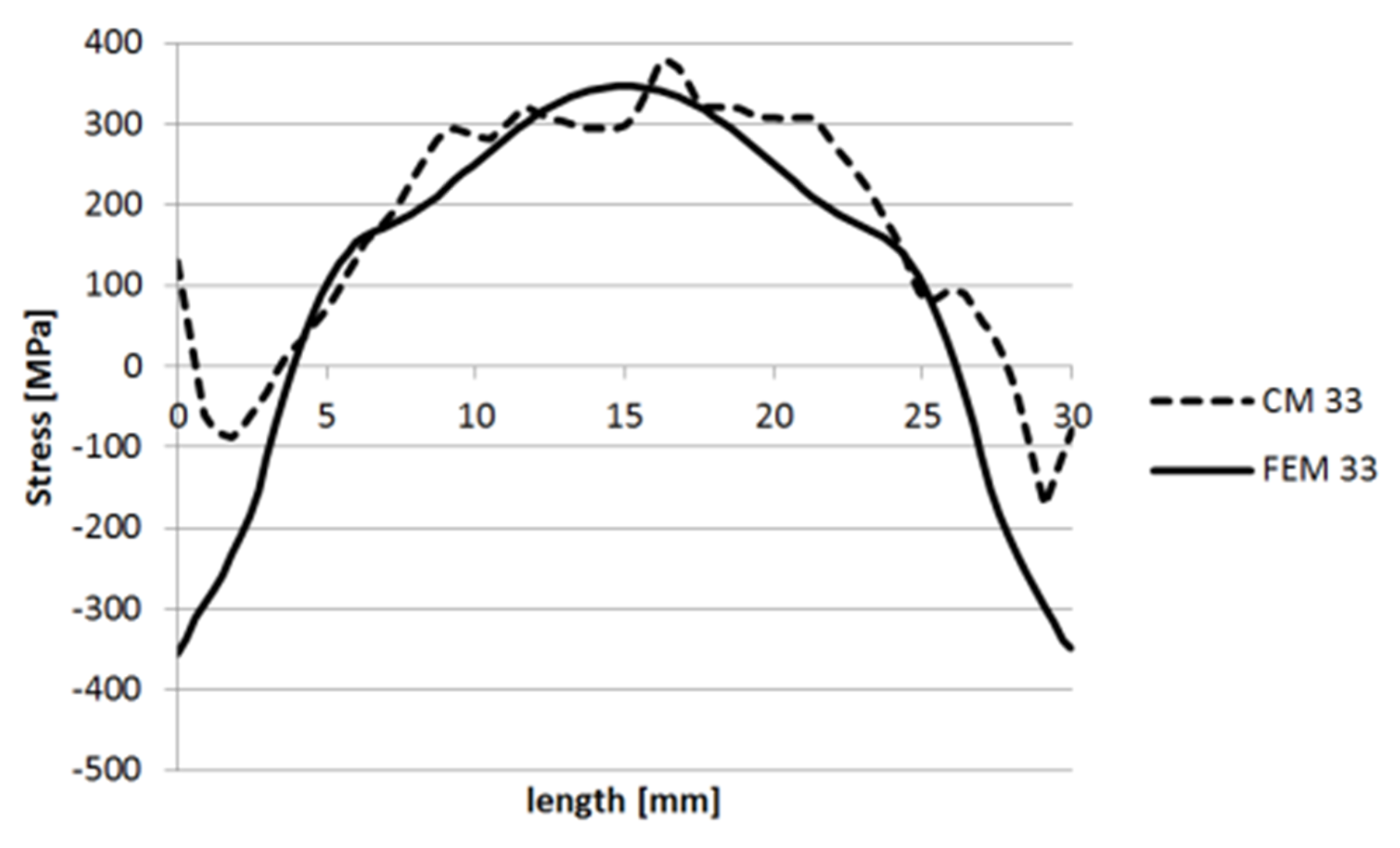
The contour method and FE analysis data were compared for line segments AB and CD indicated in Figure 38 along with the system of coordinates. Plots of the contour method and FE stresses for speciment 2 - cut 2 are shown in Figure 39, Figure 40, Figure 41, Figure 42, Figure 43 and Figure 44.

3.1.4. Specimen 3

The contour method and FE analysis data were compared for line segments AB and CD indicated in Figure 45 along with the system of coordinates. Plots of the contour method and FE stresses for speciment 3 are shown in Figure 46, Figure 47, Figure 48, Figure 49, Figure 50 and Figure 51.

3.1.5. Specimen 5

The contour method and FE analysis data were compared for line segments AB and CD indicated in Figure 52 along with the system of coordinates. Plots of the contour method and FE stresses for speciment 5 are shown in Figure 53, Figure 54, Figure 55, Figure 56, Figure 57 and Figure 58.

The values of normal stress, denoted above as direction 33 stress, determined using the contour method are in good agreement with stress values from 3D FE simulation and from neutron-diffraction measurement. This holds for almost all specimens (see Figure 36, Figure 37, Figure 43 and Figure 44), except specimen 1. In specimen 1, the stress level found by the contour method is approximately 100 MPa higher than the values from simulation at mid-points of the curves (see Figure 29 and Figure 30). This discrepancy can be attributed to the clamping arrangement and the different stiffnesses of the cut parts. The in-plane stress 22 is influenced by the cutting direction in specimens 1, 2 and 4. It is approximately 100 MPa higher than the simulation values at mid-points of the curves. The measured and calculated stresses on the second cut plane in specimen 2 (see Figure 43 and Figure 44) are offset along the x axis. This is due to the specimen having been clamped on one side only for cutting.

The best results for all stress values were obtained with specimen 3. This is consistent with the principle of the contour method which accounts for normal stresses. The stress level values along the cut plane perimeter found by the contour method cannot be considered correct because the near-edge regions are prone to error and the data must be corrected. The other stresses (in-plane stresses on cut planes) found by the contour method are in relatively good agreement with the FE simulation.

4. Conclusions

The purpose of this study was to determine residual stresses in heat-treated cylindrical specimens of 316L steel. Using wire EDM cutting, these specimens were cut along symmetry planes and non-symmetry planes. The specimens were clamped in the simplest manner possible. Nevertheless, the results were carefully evaluated, and relevant recommendations were developed. As opposed to the conventional procedure for the contour method, the specimens were only clamped on one side during cutting. This is a simpler arrangement for wire EDM cutting. It was found that valid residual stress data including the whole stress tensor can be obtained using this procedure. Residual stress levels measured by neutron diffraction were in good agreement with the data from 3D FE analysis. In-plane stresses on the cut plane were investigated in this study as well. As expected, normal stresses on the cut plane found by the contour method were in good agreement with FE data in almost all specimens. In-plane stresses on the cut plane were either approx. 100 MPa higher than FE data or in good agreement with them. Naturally, these findings only basically apply with respect to this study of heat treatment. It is desirable to pursue this research further.

References

1. Withers, P.J. Recent advances in residual stress measurement. Int. J. Press. Vessel. Pip. 2008, 85, 118–127. [Google Scholar] [CrossRef]
2. Rendler, N.J.; Vigness, I. Hole-drilling strain-gage method of measuring residual stresses. Exp. Mech. 1966, 6, 577–586. [Google Scholar] [CrossRef]
3. Hodek, J.; Zemko, M.; Shykula, P. Finite Element Model of Gear Induction Hardening. In Proceedings of the 8th International Conference on Electromagnetic Processing of Materials, Cannes, France, 12–16 October 2015. [Google Scholar]
4. Schajer, G.S. (Ed.) Practical Residual Stress Measurement Methods; Wiley: Chichester, UK, 2013; Chapter 5; pp. 109–138. [Google Scholar]
5. Hosseinzadeh, F.; Kowal, J.; Bouchard, P.J. Towards good practice guidelines for the contour method of residual stress measurement. J. Eng. 2014, 2014, 453–468. [Google Scholar] [CrossRef]
6. Johnson, G. Residual Stress Measurements Using the Contour Method. Ph.D. Thesis, University of Manchester, Manchester, UK, 2008. [Google Scholar]
7. Džugan, J.; Spaniel, M.; Prantl, A.; Konopík, P.; Růžička, J.; Kuzelka, J. Identification of ductile damage parameters for pressure vessel steel. Nucl. Eng. Des. 2018, 372–380. [Google Scholar] [CrossRef]
8. AchouriI, A.; Bouchard, P.J.; Kabra, S.; Hosseinzadeh, F. Asymmetric cuts in the contour method for residual stress measurement. In Proceedings of the 7th International Conference on Mechanics and Materials in Design, Albufeira, Portugal, 11–15 June 2017. [Google Scholar]
9. Prime, M.B.; Kastengren, A.L. The contour method cutting assumption: Error minimization and correction. In Experimental and Applied Mechanics; Springer: New York, NY, USA, 2011; Volume 6, pp. 233–250. [Google Scholar]
10. Sun, Y.L.; Roy, M.; Vasileiou, A.; Smith, M.; Francis, J.; Hosseinzadeh, F. Evaluation of errors associated with cutting-induced plasticity in residual stress measurements using the contour method. Exp. Mech. 2017, 57, 719–734. [Google Scholar] [CrossRef] [PubMed]
11. Hutchings, M.T.; Withers, P.J.; Holden, T.M.; Lorentzen, T. Introduction to the Characterization of Residual Stress by Neutron Diffraction; CRC Press: Boca Raton, FL, USA, 2005. [Google Scholar]
12. GNU OCTAVE, Version 4.0.0. Available online: https://octave.org/doc/interpreter/ (accessed on 20 October 2017).
13. JMatPro, Version 10. Available online: https://www.sentesoftware.co.uk/ (accessed on 20 October 2017).
14. Poláková, I.; Kubina, T. Flow stress determination methods for numerical modelling. In Proceedings of the 22nd International Conference on Metallurgy and materials, Brno, Czech Republic, 15–17 May 2013; p. 17. [Google Scholar]
15. MARC MENTAT, Version 2017.1.0. Available online: http://www.mscsoftware.com/product/marc (accessed on 20 October 2017).
16. Mikula, P.; Strunz, P. The Use of Thermal Neutron Beams at Medium Power Reactor LWR-15 in Řež for Competetive Neutron Research. In Proceedings of the International Conference on Research Reactors: Safe Management and Effective Utilization, Vienna, Austria, 16–20 November 2015; p. 35. [Google Scholar]
17. Pagliaro, P.; Prime, M.B.; Robinson, J.S.; Clausen, B.; Swenson, H.; Steinzig, M.; Zuccarello, B. Measuring inaccessible residual stresses using multiple methods and superposition. Exp. Mech. 2011, 51, 1123–1134. [Google Scholar] [CrossRef]
18. Kartal, M.E.; Liljedahl, C.; Gungor, S.; Edwards, L.; Fitzpatrick, M. Determination of the complete residual stress tensor in VPPA weld using the multi-axial contour method. Acta Mater. 2008, 56, 4417–4428. [Google Scholar] [CrossRef]
19. Navalho, D.; Deus, A.M.; Infante, V. Residual Stresses Due to Quenching in Aluminum Forging Parts for Aerospace Applications: Finite Element Analysis and Contour Method Measurement. In Proceedings of the 6th International Quenching and Control of Distortion Conference American Society for Metals, Chicago, IL, USA, 9–13 September 2012. [Google Scholar]
Figure 1. Schematic representation of the contour method: (a) original residual stress distribution; (b) part cut in half; (c) cut surface forced back to original position
Metals 09 01104 g001
Figure 2. Heat treatment in a furnace
Metals 09 01104 g002
Figure 3. Cooling of specimens
Metals 09 01104 g003
Figure 4. Cut-up plan for cylindrical specimens.
Metals 09 01104 g004
Figure 5. Cut-up specimens.
Metals 09 01104 g005
Figure 6. Method of clamping specimen 1 for wire EDM cutting.
Metals 09 01104 g006
Figure 7. Heat treatment in a furnace.
Metals 09 01104 g007
Figure 8. Cooling of specimens.
Metals 09 01104 g008
Figure 9. Cooling of specimens.
Metals 09 01104 g009
Figure 10. Flow stress curves as a function of temperature for ε ˙ = 0.0001 s 1 .
Metals 09 01104 g010
Figure 11. Detail of the FE mesh.
Metals 09 01104 g011
Figure 12. Temperature measurement setup.
Metals 09 01104 g012
Figure 13. A schematic sketch of the SPN100 instrument for mapping residual stresses in polycrystalline materials [16].
Metals 09 01104 g013
Figure 14. Schematic illustration of planes and directions of measurement.
Metals 09 01104 g014
Figure 15. Radial stress—central plane.
Metals 09 01104 g015
Figure 16. Hoop stress—central plane.
Metals 09 01104 g016
Figure 17. Axial stress—central plane.
Metals 09 01104 g017
Figure 18. Stress 11—FE heat treatment.
Metals 09 01104 g018
Figure 19. Stress 22—FE heat treatment.
Metals 09 01104 g019
Figure 20. Stress 33—FEM heat treatment.
Metals 09 01104 g020
Figure 21. Stress 11—CM.
Metals 09 01104 g021
Figure 22. Stress 22—CM.
Metals 09 01104 g022
Figure 23. Stress 33—CM.
Metals 09 01104 g023
Figure 24. Specimen 1—line segments used for comparing the stress levels.
Metals 09 01104 g024
Figure 25. Stress levels in 11 direction along the AB line segment.
Metals 09 01104 g025
Figure 26. Stress levels in 11 direction along the CD line segment.
Metals 09 01104 g026
Figure 27. Stress levels in 22 direction along the AB line segment.
Metals 09 01104 g027
Figure 28. Stress levels in 22 direction along the CD line segment.
Metals 09 01104 g028
Figure 29. Stress levels in 33 direction along the AB line segment.
Metals 09 01104 g029
Figure 30. Stress levels in 33 direction along the CD line segment.
Metals 09 01104 g030
Figure 31. Specimen 2—line segments used for comparing stress levels on planes of cut 1.
Metals 09 01104 g031
Figure 32. Stress levels in 11 direction along the AB line segment.
Metals 09 01104 g032
Figure 33. Stress levels in 11 direction along the CD line segment.
Metals 09 01104 g033
Figure 34. Stress levels in 22 direction along the AB line segment.
Metals 09 01104 g034
Figure 35. Stress levels in 22 direction along the CD line segment.
Metals 09 01104 g035
Figure 36. Stress levels in 33 direction along the AB line segment.
Metals 09 01104 g036
Figure 37. Stress levels in 33 direction along the CD line segment.
Metals 09 01104 g037
Figure 38. Specimen 2—line segments used for comparing stress levels on the planes of cut 2.
Metals 09 01104 g038
Figure 39. Stress levels in 11 direction along the AB line segment.
Metals 09 01104 g039
Figure 40. Stress levels in 11 direction along the CD line segment.
Metals 09 01104 g040
Figure 41. Stress levels in 22 direction along the AB line segment.
Metals 09 01104 g041
Figure 42. Stress levels in 22 direction along the CD line segment.
Metals 09 01104 g042
Figure 43. Stress levels in 33 direction along the AB line segment.
Metals 09 01104 g043
Figure 44. Stress levels in 33 direction along the CD line segment.
Metals 09 01104 g044
Figure 45. Specimen 3—line segments used for comparing the stress levels.
Metals 09 01104 g045
Figure 46. Stress levels in 11 direction along the AB line segment.
Metals 09 01104 g046
Figure 47. Stress levels in 11 direction along the CD line segment.
Metals 09 01104 g047
Figure 48. Stress levels in 22 direction along the AB line segment.
Metals 09 01104 g048
Figure 49. Stress levels in 22 direction along the CD line segment.
Metals 09 01104 g049
Figure 50. Stress levels in 33 direction along the AB line segment.
Metals 09 01104 g050
Figure 51. Stress levels in 33 direction along the CD line segment.
Metals 09 01104 g051
Figure 52. Specimen 5—line segments used for comparing stress levels on cut plane 2.
Metals 09 01104 g052
Figure 53. Stress levels in 11 direction along the AB line segment.
Metals 09 01104 g053
Figure 54. Stress levels in 11 direction along the CD line segment.
Metals 09 01104 g054
Figure 55. Stress levels in 22 direction along the AB line segment.
Metals 09 01104 g055
Figure 56. Stress levels in 22 direction along the CD line segment.
Metals 09 01104 g056
Figure 57. Stress levels in 33 direction along the AB line segment.
Metals 09 01104 g057
Figure 58. Stress levels in 33 direction along the CD line segment.
Metals 09 01104 g058