Three-Dimensional Numerical Modeling of Macrosegregation in Continuously Cast Billets

Abstract

Macrosegregation, serving as a major defect in billets, can severely degrade material homogeneity. Better understanding of the physical characteristics of macrosegregation through numerical simulation could significantly contribute to the segregation control. The main purpose of this study was to predict macrosegregation in continuously cast billets with a newly developed three-dimensional macrosegregation model. The fluid flow, solidification, and solute transport in the entire billet region were solved and analyzed. Flow patterns, revealing a typical melt recirculation at the upper region of mold and thermosolutal convection at the secondary cooling zone, significantly affect the solidification and solute distribution. The solute redistribution occurring with thermosolutal convection at the solidification front contributes significantly to continued macrosegregation as solidification proceeds. The results of this study show that the equilibrium partition coefficient is mostly responsible for the magnitude of macrosegregation, while comparison between solute P and S indicated that diffusion coefficients also have some amount of influence. Typical macrosegregation patterns containing a positively segregated peak at the centerline and negatively segregated minima at either side were obtained via the proposed three-dimensional macrosegregation model, which validated by the measured surface temperatures and segregation degree.

1. Introduction

Macrosegregation is one of the major defects in continuously cast billets, especially for high-carbon steel. It can severely degrade material homogeneity and thus affect the final properties and performance of billet-based products. Macrosegregation is also known as the main cause of cup fracture during wire cord drawing due to the formation of martensite and carbide networks [1]. Macrosegregation cannot be eliminated entirely during heat treatment, so preventing it in the casting process is crucial [2]. It is of considerable practical significance to analyze the solute distribution in castings to understand the basic physical mechanisms involved in macrosegregation.

Flemings et al. [3] first discovered the importance of convection within the mushy zone during alloy solidification and proposed the Local Solute Redistribution Equation (LSRE) to numerically study the macrosegregation caused by interdendritic flow. The flow of interdendritic liquid was modeled with a fixed dendritic solid network ignoring the effect of mushy zone. Mehrabian et al. [4] applied Darcy’s law in Flemings’ model by treating the mushy zone as a porous medium, and then established a new model for interdendritic flow behavior and the resulting macrosegregation during ingot solidification. An essential characteristic of solidification is the temperature field; the thermally induced flow exerts a significant effect on macrosegregation, but is simplified as a single measurement or assumption in Flemings’s and Mehrabian’s models. Fujii et al. [5] proposed a coupled model to solve the momentum equation and the energy equation simultaneously. The occurrence of channel-type segregation was successfully predicted in an ingot using this model. Macrosegregation is formed as solidification occurs, and the alloy solidification system is essentially a multiphase system, so a comprehensive model is required to solve the solute transport equation along with the Navier–Stokes and energy equations. Researchers studying macrosegregation models have established the continuum model [6,7] and volume-averaged model [8,9]. Bennon and Incropera [6] derived a continuum model for momentum, heat, and species transport in binary solid–liquid phase systems by integrating the microscopic descriptions of transport behavior with semi-empirical laws and principles of classical mixture theory. Poole et al. [7] developed a mathematical model for predicting solidification and segregation of binary alloys undergoing electromagnetic stirring based on the continuum model. The computed macrosegregation results for Al-4.5 pct Cu alloy were validated by the experimental measurements. A two-phase model [8] for predicting transport phenomena during the alloys solidification was developed based on the volume-averaged technique; the model was successfully used to predict the macrosegregation in industrial steel ingots [10,11]. Li et al. [10] numerically studied the species transport and macrosegregation in heavy steel ingots with a two-phase multi-scale macrosegregation model, which involved heat transfer, fluid flow, solute transport, and equiaxed grain motion on a system scale, as well as grain nucleation and growth on a microscopic scale. The macrosegregation patterns in heavy steel ingots were well reproduced with the two-phase model. Wu and Ludwig [12] developed a three-phase model for mixed columnar-equiaxed solidification and solved the conservation equations of mass, momentum, species, and energy with a Eulerian approach in a steel ingot. In a recent study [13], a dendritic model with the consideration of heat transfer, solute transport, fluid flow, grain nucleation and growth, and crystal sedimentation was applied to predict macrosegregation in a large-scale casting.

Although the foregoing models have been successfully applied in the prediction of macrosegregation during alloy solidification, the investigations mostly focus on ingot casting systems. For continuous casting processes, multi-scale modeling of macrosegregation is still highly challenging due to the complicated macro-scale transport phenomena, and a set of conservation equations must be solved over the entire region between the meniscus and sump bottom. Limited researches revealing the evolution of macrosegregation in strands were performed with two-dimensional (2D) models [14] or three-dimensional (3D) plus 2D hybrid models [15]. The 3D effect may have an influence on strand velocity and therefore on the solidification and macrosegregation patterns inside the billets, especially for the flow characteristics near the corners compared to the 2D plane. Yang et al. [16] numerically studied the transport phenomena, including fluid flow, heat transfer, and solute distribution in slab continuous casting process with a 3D coupled model. Recently, Fang et al. [17] investigated the effects of EMS induced flow on solidification and solute transport in bloom mold using a 3D numerical model. However, both researches focus only on the transport phenomena in strand mold.

The main purpose of this study was to predict the macrosegregation in continuously cast billets with a 3D macrosegregation model, which developed based on the continuum model originally proposed by Bennon and Incropera [6]. The continuum model was modified to incorporate the low Reynolds number $k-\epsilon$ turbulence model and Voller–Beckermann microsegregation model [18]. The fluid flow, heat transfer, and solute transport in the entire billet region between the meniscus and sump bottom can be solved with the 3D coupled model simultaneously.

2. Model Formulation

2.1. Assumptions

A 3D coupled model was developed to incorporate the low Reynolds number $k-\epsilon$ turbulence model and Voller–Beckermann microsegregation model based on the following assumptions.

(a)

An incompressible Newtonian fluid was assumed and the effects of turbulence were approximated with the low Reynolds number $k-\epsilon$ turbulence model.

(b)

Homogeneous and isotropic properties were assumed for steel in the simulation.

(c)

Local thermodynamic equilibrium was assumed at the solid–liquid interface.

(d)

The densities of liquid and solid were assumed to be constant and equal. Thus, the macrosegregation induced by shrinkage was not considered.

(e)

The effect of strand deformation (bulging [19]) and pore formation on the solute distribution was neglected.

(f)

Only the influence of billet curvature on macrosegregation was considered, and the force resulting from bending was ignored. The solid velocity in the whole computational domain was assumed to be equal to the casting speed.

(g)

The effects of remelting and sedimentation of grains on the segregation calculation were neglected.

2.2. Conservation Equations

The coupled model governing the conservation of mass, momentum, energy, and species, simultaneously valid in the liquid, mushy, and solid zones, can be expressed as follows.

2.2.1. Continuity Equation

$$\nabla \cdot (\rho \overrightarrow{u})=0$$

(1)

where $\rho$ and $\overrightarrow{u}$ represent mixture density and velocity, respectively, and they are defined using mass fractions $f_n$ and volume fractions $g_n$ for solid ($n=s$) and liquid ($n=l$) phases.

$$\overrightarrow{u}=f_s{\overrightarrow{u}}_s+f_l{\overrightarrow{u}}_l$$

(2)

$$\rho =g_s{\rho }_s+g_l{\rho }_l$$

(3)

However, as the densities of liquid and solid were assumed to be constant and equal, the volume fractions for solid and liquid are equal to the corresponding mass fractions.

2.2.2. Momentum Equation

$$\frac{\partial \left(\rho \overrightarrow{u}\right)}{\partial t}+\nabla \cdot \left(\rho \overrightarrow{u}\overrightarrow{u}\right)=\nabla \cdot \left({\mu }_{eff}\nabla \overrightarrow{u}\right)-\nabla p+\rho \overrightarrow{g}+S_u$$

(4)

where ${\overrightarrow{u}}_s$ represents the solid velocity, $p$ is the pressure, and the effective viscosity ${\mu }_{eff}$ describing the sum of laminar and turbulent viscosity was defined to take into account the turbulence effect. The source term $S_u$ can be described as follows:

$$S_u=\rho \overrightarrow{g}\left[{\beta }_T\left(T-T_R\right)+{\beta }_{C,i}\left(C_i-C_{R,i}\right)\right]+\frac{{\left(1-f_l\right)}^2}{f_l^3+\xi }{A}_m\left(\overrightarrow{u}-{\overrightarrow{u}}_s\right)$$

(5)

where ${\beta }_T$ and ${\beta }_{C,i}$ represent the thermal and solutal expansion coefficients, respectively, $T$ is temperature, $C_i$ is concentration of element $i$, the subscript R identifies the reference value, and $\xi$ is a very small positive number.

The first term on the right-hand of Equation (5) accounts for the thermal and solutal buoyancy, which resulted from the temperature gradient and concentration gradient during solidification. The two buoyancy terms were calculated with the Boussinesq approximation. The second term represents the phase interaction force in the mushy zone, which was modeled as a porous medium wherein the Darcy’s law can be applied. $A_m$ is permeability coefficient, which depends on the morphology of porous media. In this work, $A_m$ is calculated using the expression given by Minakawa [15] as $A_m=180/{\lambda }_2^2$, where ${\lambda }_2$ represents the secondary dendrite arm spacing and the expression [20] used here will be presented in the species equation.

2.2.3. Turbulence Model

To consider the effects of turbulence on the fluid flow and macrosegregation in upper part of mold, the low-Reynolds number $k-\epsilon$ model [21,22] was adopted here, which considered to be preferable than standard two-equation $k-\epsilon$ model or high-Reynolds number $k-\epsilon$ model in continuous casting processes. Governing equations of the model can be written as follows:

$$\frac{\partial k}{\partial t}+\nabla \cdot \left(\rho \overrightarrow{u}k\right)=\nabla \cdot \left[\left(\mu +\frac{{\mu }_t}{{\sigma }_k}\right)\nabla k\right]+G_k-\rho \epsilon +\rho D+S_k$$

(6)

$$\frac{\partial \epsilon }{\partial t}+\nabla \cdot \left(\rho \overrightarrow{u}\epsilon \right)=\nabla \cdot \left[\left(\mu +\frac{{\mu }_t}{{\sigma }_{\epsilon }}\right)\nabla \epsilon \right]+C_1{f}_1{G}_k\rho \frac{\epsilon }{k}-C_2{f}_2\rho \frac{{\epsilon }^2}{k}+\rho E+S_{\epsilon }$$

(7)

where $k$ and $\epsilon$ are the turbulent kinetic energy and its rate of dissipation, respectively. $S_k$ and $S_{\epsilon }$ represent the source terms for $k$ and $\epsilon$ equations, which related to solidification as $S_k=\frac{1-f_l^2}{f_l^3+\xi }{A}_{m}k$, and $S_{\epsilon }=\frac{1-f_l^2}{f_l^3+\xi }{A}_m\epsilon$.

The turbulent viscosity can be calculated with the following equation:

$${\mu }_t=\rho f_{\mu }{C}_{\mu }\frac{k^2}{\epsilon }$$

(8)

The coefficients and empirical constants [22] used for the Launder–Sharma low-Reynolds number model are listed in

Table 1. Coefficients and empirical constants used for the low-Reynolds number model.

Parameters	Values	Parameters	Values
$G_k$	${\mathsf{\mu }}_{\mathrm{t}}\left(\frac{\partial u_i}{\partial x_j}+\frac{\partial u_j}{\partial x_i}\right)\frac{\partial {\mathrm{u}}_{\mathrm{i}}}{\partial {\mathrm{x}}_{\mathrm{j}}}$	$D$	$2\mu {\left(\frac{\partial (\sqrt{k})}{\partial x_i}\right)}^2$
$E$	$2\frac{\mu {\mu }_t}{\rho }{\left(\frac{{\partial }^2{u}_i}{\partial x_i\partial x_j}\right)}^2$	$f_{\mu }$	$\exp \left[-3.4/{\left(1+\frac{{\mathrm{Re}}_t}{50}\right)}^2\right]$
$C_{\mu }$	0.09	$C_2$	1.92
$f_1$	1.0	${\sigma }_k$	1.0
$f_2$	$1.0-0.3\exp \left(-{\mathrm{Re}}_t^2\right)$	${\sigma }_{\epsilon }$	1.3
$C_1$	1.44	${\mathrm{Re}}_t$	$\rho k^2/\mu \epsilon$
${\mathrm{Pr}}_{\mathrm{t}}$	0.9	$S{c}_t$	1.0

.

2.2.4. Energy Equation

$$\frac{\partial \left(\rho H\right)}{\partial t}+\nabla \cdot \left(\rho \overrightarrow{u}H\right)=\nabla \cdot \left(k_{T,eff}\nabla T\right)$$

(9)

where $k_{T,eff}$ is the effective heat conductivity, which can be described as follows:

$$k_{T,eff}=\{\begin{array}{l}{k}_{T,l}+\frac{{\mu }_t}{{\mathrm{Pr}}_t},T\ge T_l\\ k_{T,s}{f}_s+k_{T,l}{f}_l,T_s<T<T_l\\ k_{T,s},T\le T_s\end{array}$$

(10)

where $k_{T,l}$ and $k_{T,s}$ are the thermal conductivity of solid and liquid, respectively, and the turbulent Prandtl number ${\mathrm{Pr}}_t$ is listed in Table 1.

The enthalpy $H$ in the energy conversation equation can be described as a function of temperature:

$$H=H_{ref}+{\displaystyle \underset{T_{ref}}{\overset{T}{\int }}{c}_{ps}dT}+f_{l}L$$

(11)

where $c_{ps}$ is the specific heat, $H_{ref}$ is the enthalpy at reference temperature $T_{ref}$, and $L$ is the latent heat of fusion. The $f_s-T$ curve is non-linear in the alloy solidification system. However, for the limitation of the existing models, coupling the non-linear $f_s-T$ function with the macrosegregation model is still challenging. Generally, a linear $f_s-T$ function [15,17] was assumed to calculate the liquid fraction:

$$f_l=\{\begin{array}{l}1,T\ge T_l\\ \frac{T-T_s}{T_l-T_s},T_s<T<T_l\\ 0,T\le T_s\end{array}$$

(12)

where $T_l$ and $T_s$ are the liquidus and solidus temperature respectively, which can be described as follows:

$$T_l=T_f+{{\displaystyle \sum m_i\cdot C}}_i$$

(13)

$$T_s=T_f+{{\displaystyle \sum m_i\cdot C}}_i/k_{p,i}$$

(14)

where $T_f$ is the fusion temperature of pure iron, $m_i$ is the slope of liquidus line, and $k_{p,i}$ is the equilibrium partition coefficient of element $i$.

2.2.5. Species Equation

$$\begin{array}{l}\frac{\partial \left(\rho C_i\right)}{\partial t}+\nabla \cdot \left(\rho \overrightarrow{u}{C}_i\right)=\nabla \cdot \left(\rho f_s{D}_{s,i}\nabla C_{s,i}\right)+\nabla \cdot \left(f_l\left(\rho D_{l,i}+\frac{{\mu }_t}{S{c}_t}\right)\nabla C_{l,i}\right)+\\ -\nabla \cdot \left[\rho f_s\left(\overrightarrow{u}-{\overrightarrow{u}}_s\right)\left(C_{l,i}-C_{s,i}\right)\right]\end{array}$$

(15)

where $D_{s,i}$ and $D_{l,i}$ represent the solute diffusion coefficient of solid and liquid, respectively. $S{c}_t$ is the turbulent Schmidt number, as listed in Table 1. ${\overrightarrow{u}}_s$ is regarded as a constant vector, casting speed here. The mixture species concentration is defined as follows:

$$C_i=f_s{C}_{s,i}+f_l{C}_{l,i}$$

(16)

$$C_{l,i}=C_{l,i}^{*}=C_i{\left(1-\left(1-{\beta }_i{k}_{p,i}\right)\cdot f_s\right)}^{\left(k_{p,i}-1\right)/\left(1-{\beta }_i{k}_{p,i}\right)}$$

(17)

$${\beta }_i=2{{\alpha }_i}^{+}\left(1-\exp \left(-\frac{1}{{{\alpha }_i}^{+}}\right)\right)-\exp \left(-\frac{1}{2{{\alpha }_i}^{+}}\right)$$

(18)

$${\alpha }_i^{+}={\alpha }_i+{\alpha }^C$$

(19)

where ${\alpha }_i$ is the solutal Fourier number, ${\beta }_i$ is solutal back-diffusion coefficient, ${\alpha }^C$ is the additional term of Fourier number, and the value was set to be 0.1 according to the works of Voller and Beckermann [18].

$${\alpha }_i=\frac{D_{s,i}\cdot t_f}{X^2}=\frac{4D_{s,i}\cdot t_f}{{\lambda }_2^2}$$

(20)

where $t_f$ is local solidification time. $X$ is the length of the microsegregation domain at the end of solidification, which usually is taken to be equal to half the final secondary dendrite arm spacing ${\lambda }_2$.

In the present work, the final secondary dendrite arm spacing, which varies with the cooling condition and alloy composition, was calculated using the empirical equations proposed by Won and Thomas [20].

$${\lambda }_2(\mu m)=\{\begin{array}{ll}(169.1-720.9\cdot C_C)\cdot C_R^{-0.4935},& 0<C_C<0.15\\ 143.9\cdot C_C^{(0.5501-1.996\cdot C_C)}\cdot C_R^{-0.3616},& C_C>0.15\end{array}$$

(21)

where $C_R$ is the cooling rate, and $C_C$ is the carbon content.

The liquidus and solidus lines of phase diagram were assumed to be straight, which means that the equilibrium partition coefficient $k_{p,i}$ is a constant. Thus, the solute redistribution at the solid–liquid interface can be described as follows:

$$C_{s,i}^{*}=k_{p,i}{C}_{l,i}^{*}$$

(22)

The solute concentration in liquid phase is equal to that at the solid–liquid interface, due to the complete diffusion was assumed in the liquid. However, the solute concentration in the solid cannot be represented by the interfacial concentration. To obtain the solute concentration in solid phase during remelting, Schneider and Beckermann [23] assumed a constant average solid concentration with the Scheil-type model, and this method is analogous to having a microscopically well mixed solid during solidification. In this study, the following equation was derived according to the Equations (16) and (22) to calculate the solid concentration:

$$C_{s,i}=\left(C_i-f_l\cdot \frac{C_{s,i}^{*}}{k_{p,i}}\right)/\left(f_s+\xi \right)$$

(23)

3. Computational Procedure

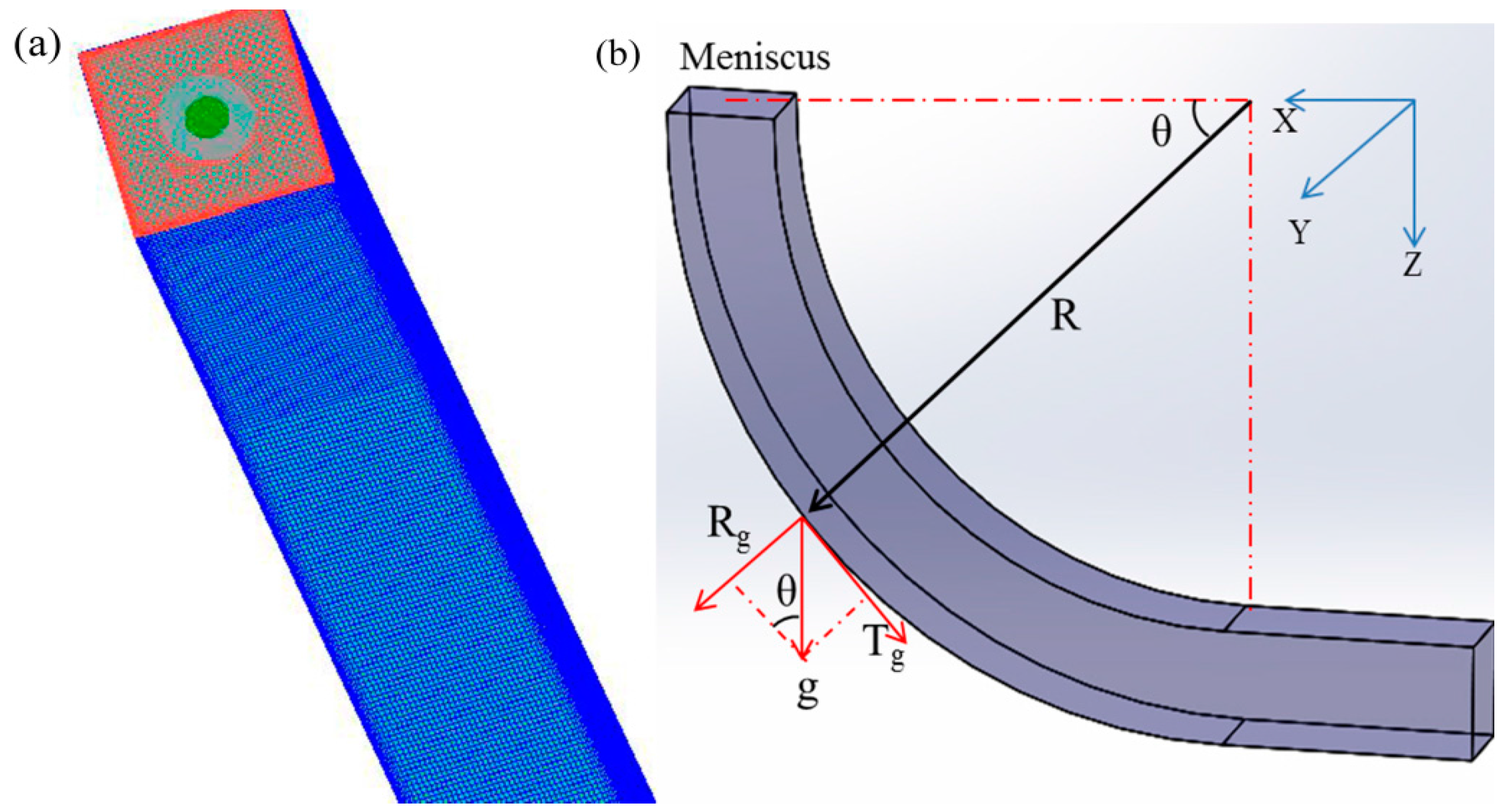
3.1. Reconstruction of Gravitational Acceleration

Continuous casting is a peculiarly complicated metallurgical process which occurs over a large region. To predict the macrosegregation in continuously cast billets, a vertical 3D geometric model (Figure 1a) was adopted to simulate the continuous casting process here. The sump bottom was determined to be about 9.4 m away from the meniscus according to the factory control software with a casting speed of 1.65 m/min. The size of the straight computational domain used here, to this effect, was designed to be 0.165 × 0.165 × 10 m³. The billet caster used in practice is a bow-type (10 m radius), and the billet curvature would influence the fluid flow and solute transport. Moreover, the major reason for liquid flow in the secondary cooling zone is reported to be thermosolutal convection, also called “double diffusive convection”, which occurs as a result of the interaction between thermal and solutal gradient. Solute redistribution and solidification in the mushy zone result in thermosolutal buoyancy, which in turn affects the formation of further macrosegregation in the billet. As reflected in Equation (5), gravity plays an important role in the calculation of thermosolutal buoyancy. The influence of gravity varies with billet curvature, which can be described with the following variable $\theta$. Thus, a reconstructed gravitational acceleration related to the variable $\theta$ was developed containing a x-component and a z-component according to the caster characteristics in this work. The reconstructed acceleration allows the consideration of billet curvature in the calculation of thermosolutal buoyancy with the straight computational domain shown in Figure 1a.

For the bow-type caster, the gravitational acceleration can be divided into radial ${\overrightarrow{R}}_g$ and tangential ${\overrightarrow{T}}_g$ components, as shown in Figure 1b. The components and variable $\theta$ can be calculated as follows:

$$\theta =\frac{\left|{\overrightarrow{u}}_c\right|t}{60R},{\overrightarrow{R}}_g=\overrightarrow{g}\cdot \sin \theta ,{\overrightarrow{T}}_g=\overrightarrow{g}\cdot \cos \theta$$

(24)

Considering the feature of straight computational domain and gravitational acceleration, two accelerations ${\overrightarrow{A}}_x$ and ${\overrightarrow{A}}_z$ are defined here: ${\overrightarrow{A}}_x=(-9.8,0,0)m/s^2,{\overrightarrow{A}}_z=(0,0,-9.8)m/s^2$. In the simulation, the decreasing direction of X was defined as the outer arc of billet caster. Then, the reconstructed gravitational acceleration applied in the calculation of thermosolutal buoyancy can be described as follows:

$${\overrightarrow{A}}_r={\overrightarrow{A}}_x\cdot \sin \theta +{\overrightarrow{A}}_z\cdot \cos \theta$$

(25)

3.2. Numerical Scheme

The macrosegregation model was solved in the computational domain shown in Figure 1 with the appropriate initial conditions, boundary conditions, and thermophysical parameters in open-source software OpenFOAM; details of the conditions can be found in previous work [24]. The high-carbon steel SWRH82B is used in this study, the chemical composition and corresponding diffusion coefficients are listed in

Table 2. Chemical compositions and corresponding coefficients.

Element	${\mathit{C}}_{0,\mathit{i}}$ (wt %)	${\mathit{k}}_{\mathit{p},\mathit{i}}$ (-)	${\mathit{\beta }}_{\mathit{C},\mathit{i}}$ (1/wt %)	${\mathit{D}}_{\mathit{s},\mathit{i}}$ (m2/s)	${\mathit{D}}_{\mathit{l},\mathit{i}}$ (m2/s)
C	0.81	0.34	0.0110	$7.61\times {10}^{-6}\exp (-\mathrm{134,557.44}/RT)$	$5.2\times {10}^{-7}\exp (-\mathrm{11,700}/RT)$
Si	0.19	0.52	0.0119	$3.0\times {10}^{-5}\exp (-\mathrm{251,458.4}/RT)$	$5.14\times {10}^{-8}\exp (-9150/RT)$
Mn	0.8	0.78	0.0019	$5.5\times {10}^{-6}\exp (-\mathrm{249,366.4}/RT)$	$3.18\times {10}^{-7}\exp (-\mathrm{16,600}/RT)$
P	0.015	0.13	0.0115	$1.0\times {10}^{-6}\exp (-\mathrm{182,840.8}/RT)$	$1.35\times {10}^{-6}\exp (-\mathrm{23,700}/RT)$
S	0.008	0.035	0.0123	$2.4\times {10}^{-4}\exp (-\mathrm{223,425.6}/RT)$	$4.9\times {10}^{-8}\exp (-8600/RT)$

along with the equilibrium partition coefficients of each element, and the thermophysical parameters of the steel are listed in

Table 3. Operation parameters and thermophysical parameters.

Parameters	Values
Casting speed, m/min	1.65
Pouring temperature, K	1758
Mold length, m	0.8
Length of secondary cooling zone, m	6.65
Length of air cooling zone, m	2.55
SEN depth from meniscus, m	0.1
SEN inner diameter, m	0.035
SEN outer diameter, m	0.075
Density, kg/m3	7340
Solid specific heat, J/(kg·K)	650
Liquid thermal conductivity, W/(m·K)	33.5
Solid thermal conductivity, W/(m·K)	24.7
Thermal expansion coefficient, K−1	2.0 × 10−4
Liquid viscosity, Pa·s	0.00461
Latent heat, J/kg	231,637
Fusion temperature of pure iron, K	1808

. The finite volume method (FVM) was applied to the set of macroscopic transport equations, providing temperature and concentration fields as input parameters for the microsegregation model. The dendritic structure, liquid fraction, and solute distribution at the solidification front calculated by the microscopic model were reapplied to the macrosegregation model to update the flow, temperature, and concentration field values. The large time-step transient solver, PIMPLE (a merged PISO-SIMPLE algorithm), was used to solve the pressure-velocity coupling; this algorithm has shown superior numerical stability in large time-steps calculations as compared to the Pressure Implicit Splitting Operator (PISO) algorithm [25], which is applied in the PIMPLE algorithm to rectify the pressure-velocity correction, while the Semi-Implicit Method for Pressure-Linked equations (SIMPLE) algorithm allowed us to calculate the pressure from velocity components on a grid by coupling Navier–Stokes equations with an iterative procedure. Both numerical stability and efficiency can be achieved with the PIMPLE algorithm. The initial time step was set at 0.001 s and was adapted gradually (increased to 0.023 s) in the solution. For each time step, the maximum iteration number was set to 600 to reduce the residual values of momentum conservation equation below 10⁻⁶, as well as the energy and species conservation equations below 10⁻⁷. About 160 h were required to perform a fully-coupled simulation with 1,587,600 grid cells on a workstation with 3.4 GHz CPU and 16 GB RAM in parallel. Grid independence analysis reported by Ge et al. [13] and Du [26] for the simulation of macrosegregation shows that the variation of grid size has little effect on the predicted segregation pattern. Thus, no grid dependence study was performed in this work.

3.3. Boundary Conditions

The boundary conditions considered applicable to the macrosegregation simulation in continuously cast billet are described as follows:

3.3.1. Meniscus

Considering the insulating effect of mold flux, the free surface was set to be adiabatic wall. The normal gradients of other variables were set to be zero.

3.3.2. Inlet and Outlet

Molten steel is poured into the mold through a straight nozzle at a certain flow rate corresponding to the casting speed. The inlet velocity profile was assumed to be flat and determined based on the inlet-outlet mass balance. Thus, boundary conditions of all variables at the inlet can be described as follows:

$$u_x=0,u_y=0,u_z=u_{in}=\frac{4w_b^2}{\pi d_{in}^2}{u}_c$$

(26)

$$T_{in}=T_c,C_{in,i}=C_{0,i}$$

(27)

where $w_b$ represents the billet width, $d_{in}$ is the SEN inner diameter, and $T_c$ is the pouring temperature. The values of $k$ and $\epsilon$ at the SEN inlet were calculated on the basis of the semi-empirical equations [27]. At outlet, fully developed condition was adopted for the fluid flow, and normal gradients of other variables were set to be zero.

3.3.3. Moving Wall

Velocity of the moving wall (billet surface) was set to equal casting speed, and the detailed thermal boundary conditions are given as follows:

(a) Mold zone:

$$q_m=a-b\sqrt{L_z/u_c}$$

(28)

where $a$ is a constant, which value is set to be 2,680,000 $W/m^2$, and $b$ is an unknown coefficient:

$$b=\frac{1.5(a-\overline{q})}{\sqrt{L_m/u_c}}$$

(29)

where $L_m$ is the mold length, and $\overline{q}$ is an unknown coefficient:

$$\overline{q}=\frac{C_W\times Q_W\times \Delta T}{S_{eff}}$$

(30)

where $C_W$ is the specific heat of water, $Q_W$ is the flow rate of cooling water, $\Delta T$ is the temperature difference of cooling water, and $S_{eff}$ is effective area of mold.

(b) Secondary cooling zone:

$$q_s=h(T_{surf}-T_W)$$

(31)

where $T_{surf}$ is the surface temperature of billet, $T_W$ is the temperature of cooling water, and $h$ is the integrative heat transfer coefficient, which can be calculated using the following equations:

Foot-roller zone [28]:

$$h=B{Q}_W^c\left(1-M\left(T_W-T_0\right)\right)$$

(32)

where the constants: B = 392.5, c = 0.55, M = 0.0075, and T₀ = 273.15 K.

Other spray zones:

$$h=m+A{Q}_W^n$$

(33)

where $m$, $A$, and $n$ are constants, $m=116W/(m^2\cdot K)$, $A=10.44$, and $n=0.851$.

(c) Air cooling zone:

$$q_a=\sigma e(T_{surf}+T_{ambi})\left(T_{surf}^2+T_{ambi}^2\right)$$

(34)

where $\sigma$ is Stefan–Boltzmann constant, $e$ is emissivity of billet surface, and $T_{ambi}$ is ambient temperature.

4. Results and Discussion

The 3D distribution of temperature, velocity, and solute element can be obtained by solving the governing equations. The flow field directly affects the solute convection, and the solidification determines the dendritic and liquid fraction distributions, then affects the redistribution of solute at solidification front, the results of solidification and flow field would be shown and discussed first.

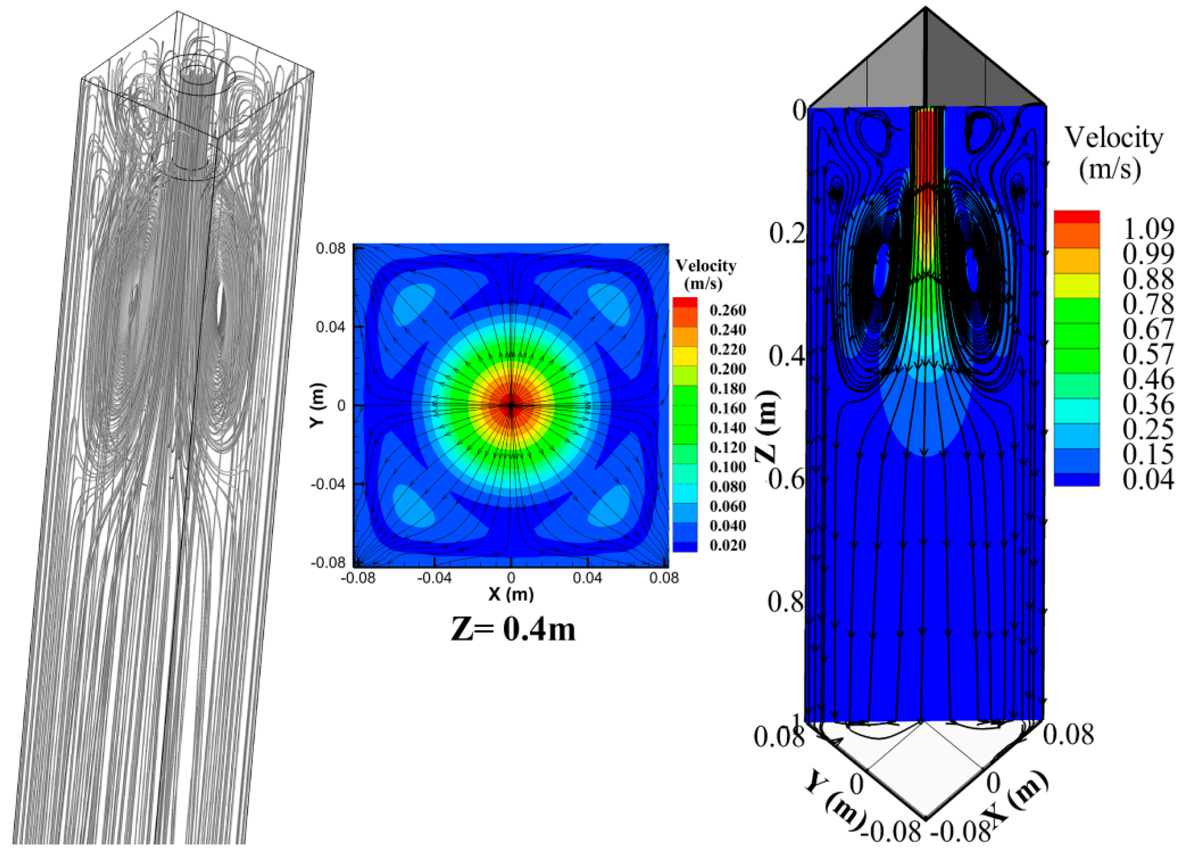
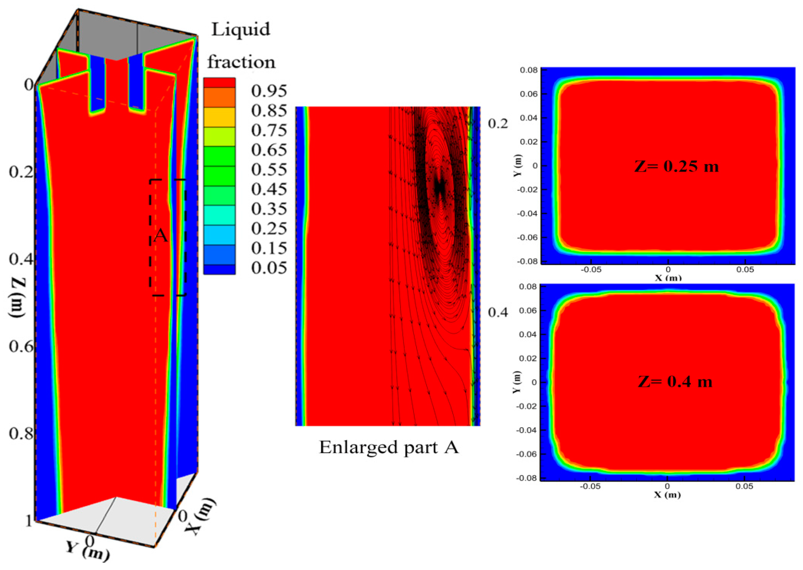
4.1. Fluid Flow and Solidification

The predicted 3D streamline distribution, detailing the flow performance of molten steel in the mold, is illustrated in Figure 2 along with the velocity contour and its corresponding streamlines on the cross section of the Z = 0.4 m plane and diagonal section. The molten steel was poured into the mold through a submerged nozzle with a certain flow rate corresponding to the casting speed. The turbulent flow formed below the nozzle in response to the impinging jet of molten steel. A portion of the molten steel flowed downward into the secondary cooling zone along the caster, while the remainder moved upward along the solidified shell. This created a significant melt recirculation around the impinging jet at the upper region of the caster. The depth of the recirculating region was about 0.45 m, as dependent on the casting speed, mold size, and geometry of the nozzle. Another relatively weak recirculation zone appeared above the large melt recirculation due to the backflow of the molten steel. The cooperation between the backflow and meniscus created the melt recirculation below meniscus, which would cause serious level fluctuation and further increase the likelihood of powder entrapment during continuous casting. The velocity distribution on the cross section (Z = 0.4 m) indicated that larger velocity occurred at the corner compared to the edge near the solidification shell. This can also be reflected in the flow characteristics indicated with streamlines on the cross section shown in Figure 2. The introduced molten steel moved out from the billet center in all directions on the cross section, and the streams focused at the billet corner. The fluid flow along the centerline was transferred to the billet corner due to the solidified shell, enhancing fluid flow at the billet corner. Flow field is the key factor during continuous casting, and it will significantly affect the energy and solute transport. The predicted 3D flow characteristics in the continuously cast billet are crucial for accurate simulation of macrosegregation.

Figure 3 shows the predicted solidification profiles, including both the center and corner of the billet surface, along the casting direction. Four surface temperatures that measured with pyrometers are also shown in the figure to validate the solidification model. In the experiment, four infrared thermometers were placed at the 2nd and 3rd zone of the second cooling zone and at two positions in the air-cooling zone. The predicted and experimental surface temperature values are in close agreement, which indicates that the solidification model used here is accurate. The simulated temperature profiles for both the surface center and corner also exhibited similar evolution characteristics: Both decrease sharply in the mold due to the high cooling intensity, then the decreased cooling intensity and release of latent heat create an increase in temperature in the secondary cooling zone. (The temperature either decreased or increased in the secondary cooling zone, but varied slightly in this region.) The difference between the temperature profiles mainly exists in the mold region, wherein the temperature at the surface corner fell below 800 K at the mold exit, while about 1200 K was obtained for the surface center. This can be attributed to the solidification characteristics of billet in the mold, wherein cooling at the corner is two-dimensional while unidimensional solidification is commonly assumed at the billet surface. The liquid fraction profile at the billet center is also shown in the figure as a function of the distance from the meniscus. The sump bottom was predicted to be 9.7 m.

Figure 4 shows the predicted liquid fraction distribution at different sections in the mold including the longitudinal section, diagonal section, and cross section of Z = 0.25 m and 0.4 m planes. As solidification proceeds, the solidified shell with a certain thickness appeared at the billet edge and then developed gradually as the distance to the meniscus increased. The simulated results indicate a thicker billet shell at the diagonal section in comparison to that at the longitudinal section. Distinctions in the liquid fraction distribution were directly revealed by the results at the cross section. About 10 mm in thickness is achieved for the distinction at the mold exit in the present work. The primary cause of that is the cooling characteristic of billet, as shown in Figure 3, which details the evolution of temperature at the billet corner and surface during continuous casting, revealing the distinctions in cooling intensity. There was a sharper variation in temperature at the surface corner compared to the center, which created a relatively larger growth rate of the solidified shell at the surface corner. The flow pattern shown in Figure 2 has indicated relatively larger velocity at the billet corner, where the fluid flow accelerated the energy transport and enhanced the development of the solidified shell. The development of billet shell at the diagonal section is relatively uniform, while the solidified shell tends to expand outwards at an axial distance about 0.4 m away from the meniscus (Figure 4, part A). The enlarged plot of part A and cross sections evidently indicate a thicker shell at the Z = 0.25 m plane in comparison to the Z = 0.4 m plane, which appears to violate the growth tendency of the solidified shell. To further explore this abnormal finding, the liquid fraction profiles at different cross sections including Z = 0.25 m, 0.40 m, and 0.60 m were analyzed, as shown in Figure 5. The thickest solidified shell appears at the Z = 0.25 m plane among these three billet locations, although with the smallest distance from the meniscus. The abnormality existing in the distribution of the solidified shell is likely related to the flow pattern of molten steel in the mold, so the work zeroed in on the streamline distribution in part A as also shown in Figure 4 to explore the flow performance in this region. As shown, the melt recirculation, which would promote the energy dissipation by increasing the effective heat conductivity and convection, mainly occurs in the region of 0.2 to 0.4 m away from the meniscus. The solidified shell developed extensively and quickly in this region in response to the increased energy dissipation, while a portion of the molten steel with large velocity flowed toward the solidified shell at the end of the impinging jet (i.e., the source of the circulation flow), leading to “washing effect”. This caused a decrease and uneven distribution of the solidified shell, as observed in the cross section of Z = 0.4 m.

Figure 6 presents the contour plots of velocity and liquid fraction at several cross sections with different distances (Z = 3 m, 5 m, 7 m, and 9 m) to the meniscus. The plots consist of both the velocity and liquid fraction at the same cross section, because the distribution of both variables was symmetrical along the Y-axis. The upper part of each plot shows the velocity distribution and the bottom details the liquid fraction. The simulation results showed consistency in the distribution of velocity and liquid fraction at the same location in the billet. The maximum velocity at the cross section decreased from 0.045 m/s to 0.029 m/s as the distance to the meniscus increased; further, it was nearly equal to the casting speed (0.0275 m/s). The maximum liquid fraction decreased from 0.8 to 0.28, and the cross-flow zone gradually shrunk as the solidification proceeds. The limited space and fluid flow shown in the figure corresponding to Z = 7 m plane were responsible for internal flaws such as segregation and porosity. Thereby some measures such as soft-reduction and electromagnetic stirring can be implemented in this region to reduce or suppress the defects. The streamline distribution at each cross section is also shown in Figure 6 to illustrate the melt circulation in flow zone, which created an asymmetrical distribution of the velocity and liquid fraction. This also exerted some influence over the solute distribution, as discussed below. The formed melt circulation shown in Figure 6, which is commonly called “thermosolutal convection” [29], was believed to be induced by thermal and solutal buoyancy.

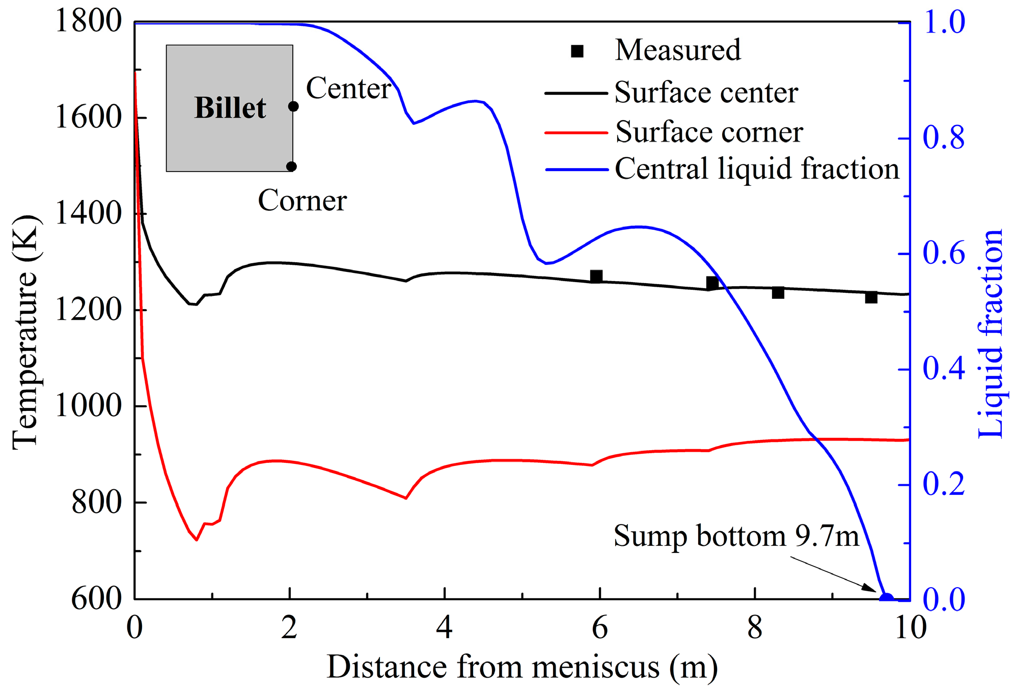
4.2. Solute Distribution and Validation

Involving the effect of thermosolutal buoyancy, solute diffusion, and convection during continuous casting process, the macrosegregation model developed here has predicted the 3D distribution of solute elements in the billet. Figure 7 shows the predicted distribution of different solute elements in mold ((a) C; (b) P; (c) S; (d) Mn), which is qualitatively similar for each element. The various elements encountered similar convection from the fluid flow and were redistributed at the solidification front. The mass fraction of elements in solid and liquid, which is controlled by the partition coefficient, is the only difference between them. For the sake of brevity, this study focuses only on the solute C to analyze the evolution of macrosegregation in the billet.

The distribution pattern of solute C, as shown in Figure 8, confirms that solute redistribution occurred in the mold due to the convection, diffusion, and solidification after the molten steel was poured into mold through the submerged nozzle. Some amount of inhomogeneity in solute distribution was observed, and this is the early stage of macrosegregation in the billet. Solidification plays an important role in solute redistribution; the predicted solidified shell in the mold is also shown in the figure as a red line for comparison. The mass fraction of solute C in the solid zone was lower than the initial value (0.81), i.e., underwent “negative segregation”, while aggregation of the solute element in the mushy zone resulted in “positive segregation” (Figure 9). The predicted profiles for the concentration of solute C and the liquid fraction at different distances to the meniscus are also shown in Figure 9. The primary cause of the segregation is believed to be solute redistribution occurring at the solidification front as solidification proceeds. The redistribution of each solute element is mainly dependent on its partition coefficient, which is usually less than 1. (Normally, there is severer segregation for smaller partition coefficients.) The equilibrium partition coefficient in Equation (22) indicates that solute elements are rejected from the solidified shell into the mushy zone, leading to compositional heterogeneity in the billet. The predicted results also show a relatively high concentration of solute C in the upper region of the mold, which can be attributed to solute redistribution and melt convection in the mold. The flow patterns shown in Figure 2 suggested that a part of the molten steel moved upward along the billet shell, forming a pair of large recirculation zones in response to the impinging jet pouring from the submerged nozzle. Consequently, the solute-enriched liquid adjacent to the billet shell would rise back to the upper zone of the mold, resulting in the high concentration zone, also leading to the negative segregation region near the billet shell.

The solute distribution changed again below the back-flow region, where positive segregation occurred in the mushy zone adjacent to the solidified shell. The prediction results also indicate a solute-enriched region at the distance of about 0.1 to 0.2 m from the meniscus. To explain this finding, the streamlines distribution in this region is also presented in Figure 8. Local positive segregation was likely a result of recirculation occurring at this region, wherein a relatively high solidification rate was achieved, followed by the mushy zone; the solute-enriched liquid was concentrated at this region as-affected by the recirculation. The “washing effect” [15,17] also created negative segregation in the mushy zone at a distance of 0.3 m from the meniscus, as shown in Figure 9a; positive segregation at the Z = 0.18 m plane and negative segregation at the 0.3 m plane were clearly identified with nearly the same liquid fraction distribution. Figure 8 also shows the distribution of solute C at different cross sections in the mold. The corresponding predicted concentration and liquid fraction profiles are shown in Figure 9b. There were similar distributions of solute C for different cross sections below the turbulent region in the mold. The segregation zone, both positive and negative, gradually moved toward the billet center as solidification progressed.

The segregation degree is defined to directly describe the solute distribution:

$$r_i=C_i/C_{0,i}$$

(35)

where, $r_i$ is segregation degree of element $i$, and $C_{0,i}$ represents the initial mass fraction.

Figure 10 shows the segregation degree of solute C near the end of solidification as predicted to be 9.7 m. Figure 10a shows contour plots of the segregation distribution at longitudinal and diagonal sections, and Figure 10b shows the segregation profiles at two distances (Z = 9.1 m and 9.9 m) from the meniscus along the X-axis and X–Y direction, respectively. There was negligible variation in the solute distribution when the ongoing solidification nearly complete. The segregation profiles showed no evident distinction between the two plotted locations for both sections, although the central liquid fraction was predicted to be about 0.2 at the Z = 9.1 m plane. This suggests that macrosegregation in the billet formed in the mushy zone with relatively low central liquid fraction, but not the region near the sump bottom and this corresponds with the conclusion reported in previous study [24]. Comparison between the segregation profiles of the two sections (longitudinal and diagonal) reveals the similar features in the distribution of solute C. The simulation results indicate that the highest segregation degree (positive segregation) occurred at the central region of billet, while relatively low values of segregation degree (negative segregation) are predicted at either side of the center. This precisely corresponds to the reported typical distribution of centerline segregation with a positively segregated peak at the centerline and negatively segregated minima at the sides [30].

As described in Equation (12), a linear $f_s-T$ function was applied in the calculation of solid fraction in this work. The nonlinear $f_s-T$ function corresponding to the Voller–Beckermann microsegregation model should be given as [31]:

$$f_s=\left(\frac{1}{1-\beta k_p}\right)\left\{1-{\left(\frac{T_f-T}{T_f-T_l}\right)}^{\left(1-\beta k_p\right)/\left(k_p-1\right)}\right\}$$

(36)

Obviously, the linear $f_s-T$ relation ignores the influence of the partition coefficients and back-diffusion coefficients, which are difficult to determine in the multicomponent alloy system (values for the coefficients vary with different elements). The distinction between the calculated solid fraction and theoretical value would cause some effects on the magnitude of segregation. To discuss this, other two two-dimensional calculations [24] were performed with the linear $f_s-T$ function (Equation (12)) and nonlinear $f_s-T$ relation (Equation (36)) separately. In the calculation, the partition coefficient in Equation (36) is determined to be 0.34, and the back-diffusion coefficient is set to be 0.9 according to the calculated values of solute C. As noted already, the coefficients are different for various solute elements. Thus, the discussion only focuses on the predicted results of solute C, which are shown in the Figure 11 with the liquid fraction profiles: (a) Z = 4 m; and (b) Z = 9.9 m. Comparison between the two calculations shows a minor distinction in the liquid fraction at mushy zone, which distinction leads to the difference in the predicted concentration of solute C. However, the influence of solid fraction calculation on the final macrosegregation patterns is shown to be small. Thus, the linear $f_s-T$ function applied in this work is acceptable. Even so, the present method of calculating the solid fraction in Voller–Beckermann microsegregation model cannot be considered realistic, and much future work is required to develop a more accurate method.

To validate the 3D macrosegregation model, solute C across the cross section of experimental billet was analyzed with a carbon-sulfur analyzer. Specimens for chemical analysis were extracted by drilling from the billet along the diagonal line; the detailed scheme of the specimens is shown in Figure 12a. The drilling specimens were 5 mm in diameter and 10 mm in depth, with a distance between specimens of 15 mm. Figure 12b gives the comparison in segregation degree profiles between the experiment and simulation, which were in close agreement, confirming the validity of the 3D macrosegregation model developed in this study.

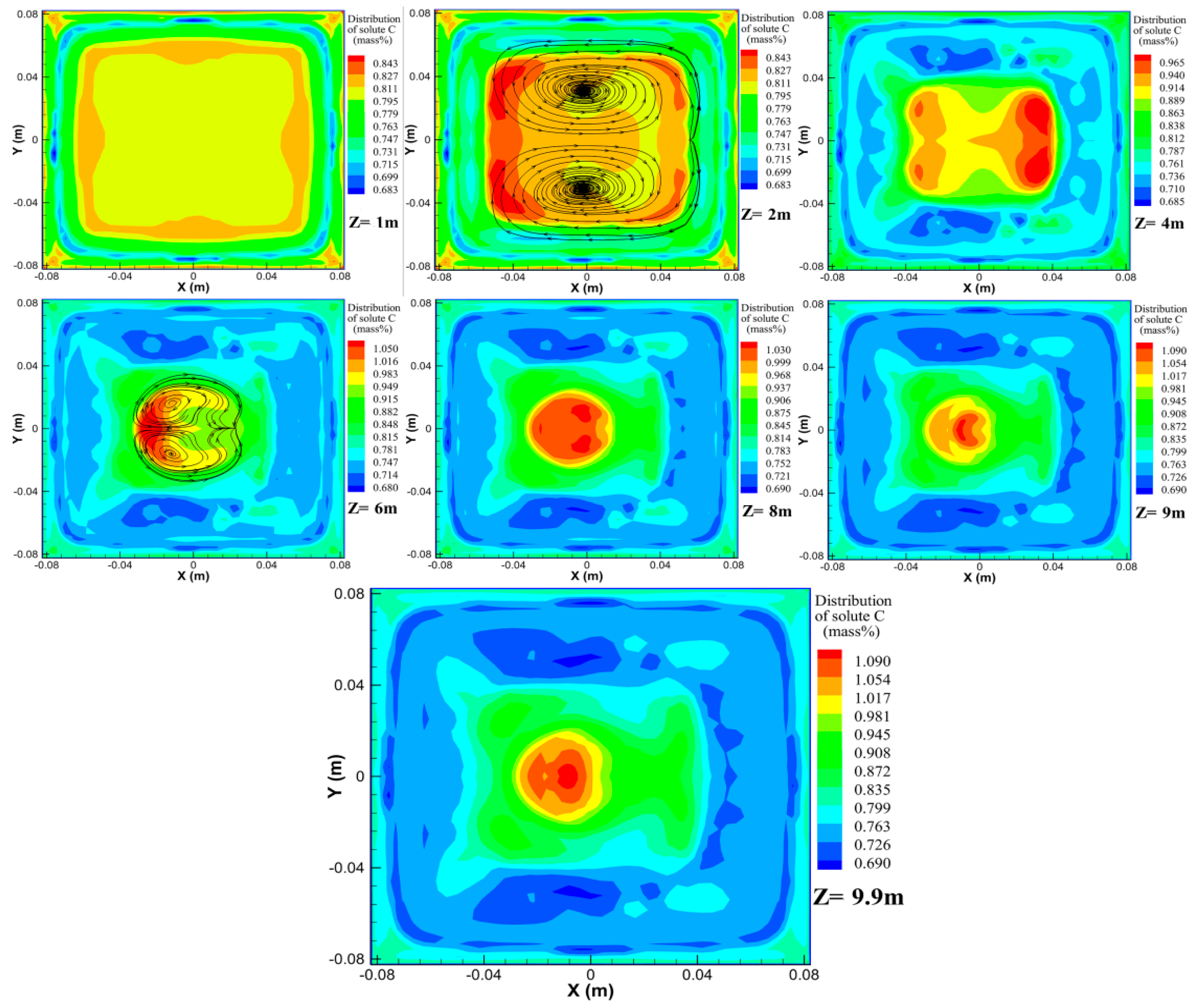
4.3. Evolution of Macrosegregation

The computed distribution pattern of solute C on the cross section at different locations of the billet, including 1, 2, 4, 6, 8, 9, and 9.9 m, is shown in Figure 13 to reveal the evolution of macrosegregation during billet continuous casting. The distribution of solute C at the billet edge was relatively uniform and barely changed in comparison to the initial distribution. This can be attributed to the high cooling rate at the billet edge, wherein the solidification was too fast for the solute redistribution. As solidification proceeds, the decreased cooling rate facilitated solute redistribution at the solidification front leading to a low solute concentration in the resulting shell and increased mass fraction in the mushy zone, as shown in the figure corresponding to the Z = 1 m plane. The ring-shaped negative segregation zone formed in response to the washing effect in the mold persisted at Z = 9.9 m plane, where accomplished solidification was achieved in the billet. This can be attributed to the solute diffusion coefficient in the solid, as described in Table 2. The limited diffusion of solute elements in the solid did not readily allow variation in the solute distribution at macroscopic scale, and this corresponds exactly to the previous report [30] that macrosegregation in cast products cannot be eliminated by subsequent hot working or annealing. The basic cause of segregation in the resulting billets is that the liquid rejects the solutes during solidification because the solid has less solubility for them as compared to the liquid. The solute rejection was simulated as solute redistribution at the solidification front controlled by the microsegregation model in this work. A solute-enriched liquid formed near the solidified shell as solidification progressed, while the resulting localized solute enrichment caused macrosegregation due to the physical movement of liquid. The thermosolutal buoyancy is believed to play an important role in this movement. The streamline patterns shown in the figure clearly indicate the ongoing thermosolutal convection of molten steel in the billet, which resulted in an uneven, large-scale, and complex solute distribution. The solute C was not equally distributed in the cross sections due to thermosolutal buoyancy and gravity. As solidification progressed, solute elements gradually gathered at the central region of the billet as the mobile molten steel decreased. Macrosegregation formed completely in response to the interaction among solidification, solute redistribution, and thermosolutal convection. It should be noted that remelting and sedimentation of grains will affect the patterns and severity of segregation, especially in continuously cast bloom and slab. Thus, new mathematical model need to be developed considering the sedimentation of grains to more accurately predict the segregation patterns in bloom and slab.

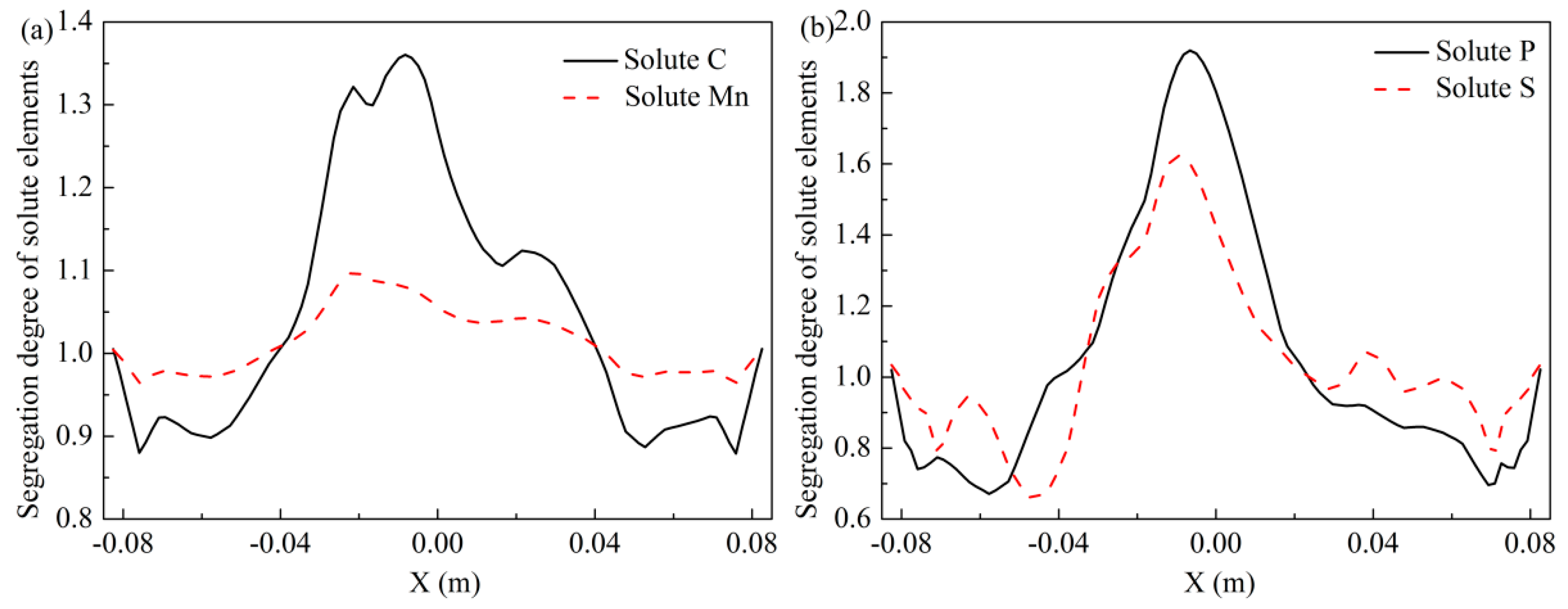
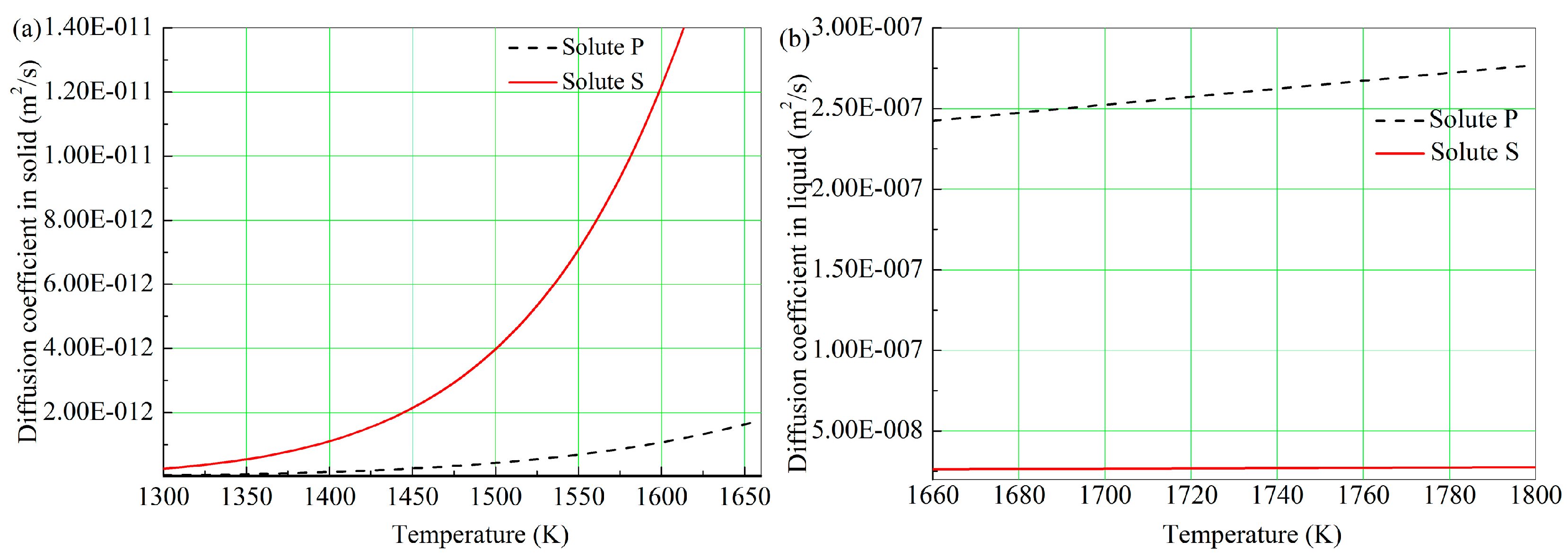
4.4. Comparison between Different Elements

Although with similar feature of segregation profile, evident distinctions in the magnitudes of segregation have been obtained through the 3D macrosegregation model for the different solute elements. Among the four typical chemical alloy elements shown in Figure 14, solute P yielded the highest segregation degree at up to 1.920. Solute Mn showed the lowest segregation degree (1.099) and solute C’s was 1.322. The equilibrium partition coefficient of various elements is the main contributor to these distinctions. Macrosegregation results from movements of micro-segregated regions over macroscopic distances due to the motion of liquid, while microsegregation arises as a result of the solute redistribution at solidification front, which is mainly controlled by the equilibrium partition coefficient. The smaller is the partition coefficient, the more disparate is the mass fraction in the liquid and solid and thus the severer is the microsegregation. Although the formation of macrosegregation is primarily affected by the natural convection due to thermal and solutal buoyancy, and partly relevant to the diffusion coefficient of solute elements, the solute redistribution occurring at the solidification front is the determining factor in the magnitudes of the macrosegregation. A smaller equilibrium partition coefficient was adopted for the solute P compared to the solute C and Mn, so severer macrosegregation was predicted for solute P. However, although with smaller equilibrium partition coefficient compared to the solute P, solute S still achieved a lower degree of segregation, due to the distinction in diffusion coefficients between the two elements. Figure 15 shows the variations in diffusion coefficients with temperature for the two elements. The diffusion coefficient of solute S in the solid is much larger than that of solute P, especially at the temperature near the solidus. Increase in diffusion coefficient contributed to the homogenization of the solute elements during solidification, where the resulting microsegregation was relatively weak according to the microsegregation model. Thus, the predicted distinctions in the segregation degree of solutes P and S are reasonable.

5. Conclusions

A 3D macrosegregation model containing both the low Reynolds number $k-\epsilon$ turbulence model and Voller–Beckermann microsegregation model was developed in this study based on the continuum model proposed by Bennon and Incropera. The solidification, fluid flow, and solute transport in the entire billet region between the meniscus and sump bottom were analyzed using this model to reach the following main conclusions.

(1)

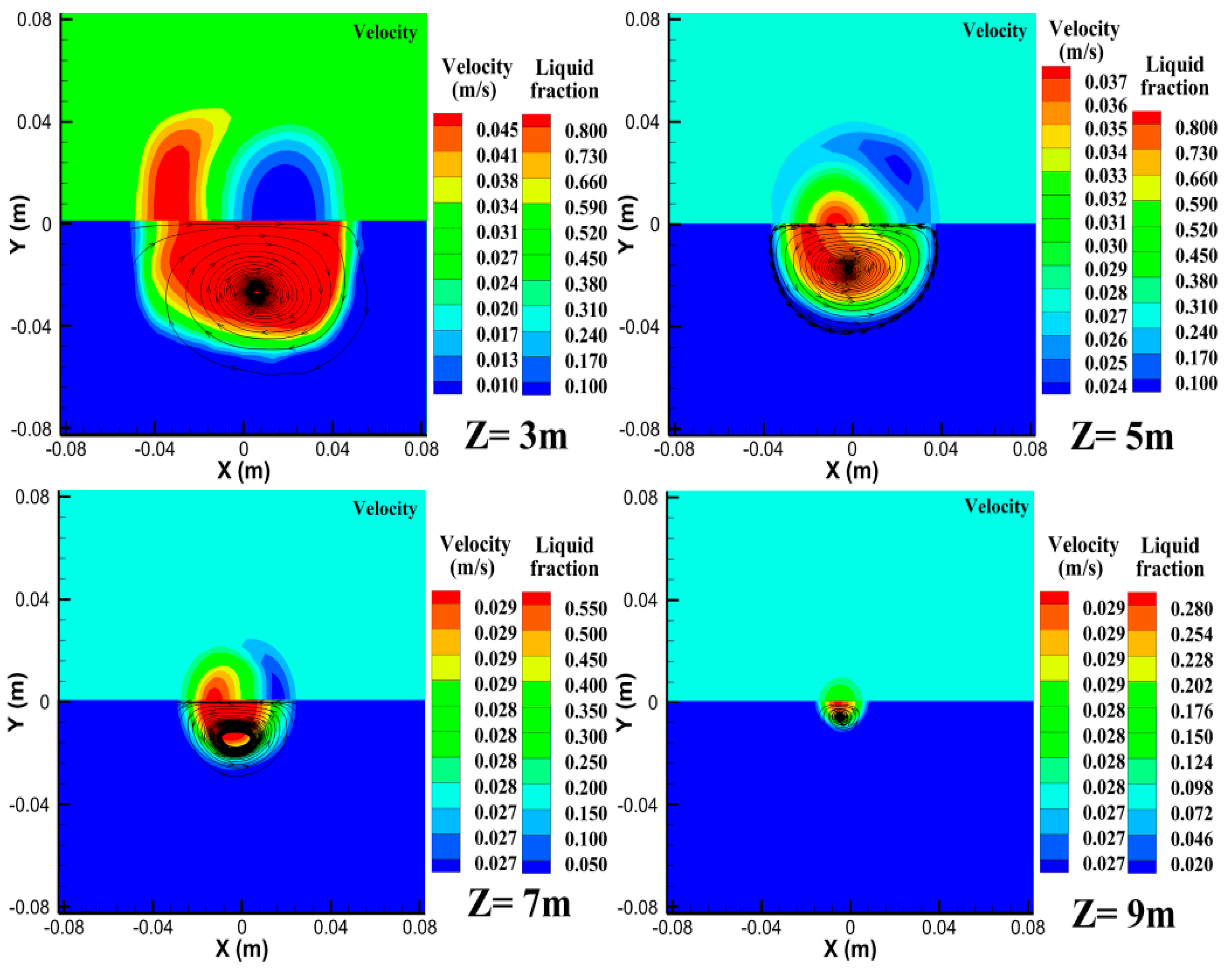
Flow patterns showed a significant melt recirculation around the impinging jet at the upper region of the mold. Two other relatively weak melt recirculation zones appeared in response to the backflow of molten steel. There was larger velocity at the corner than the edge near the solidification shell.

(2)

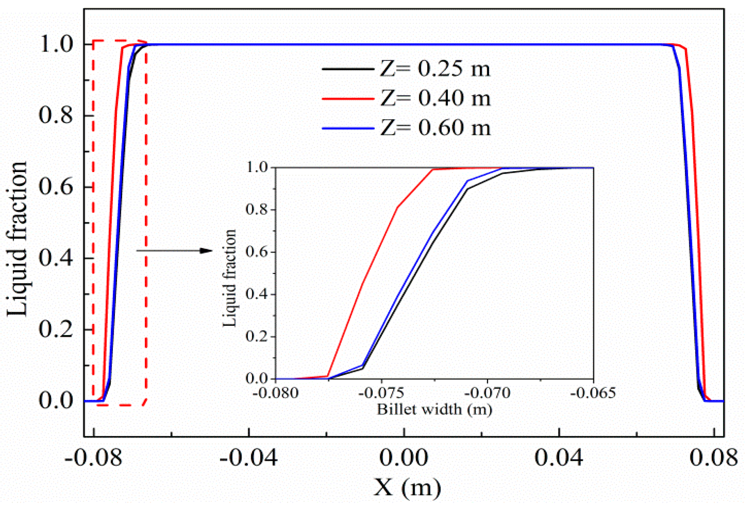
The solidification model applied in this work was validated according to surface temperature measurements. The relatively high cooling intensity created a thicker solidified shell at the diagonal section compared to the longitudinal section. Melt recirculation and washing effects further created uneven distribution of the solidified shell at the longitudinal section. The simulation results indicated thermosolutal convection at the secondary cooling zone, which resulted in asymmetrical distribution of the velocity and liquid fraction.

(3)

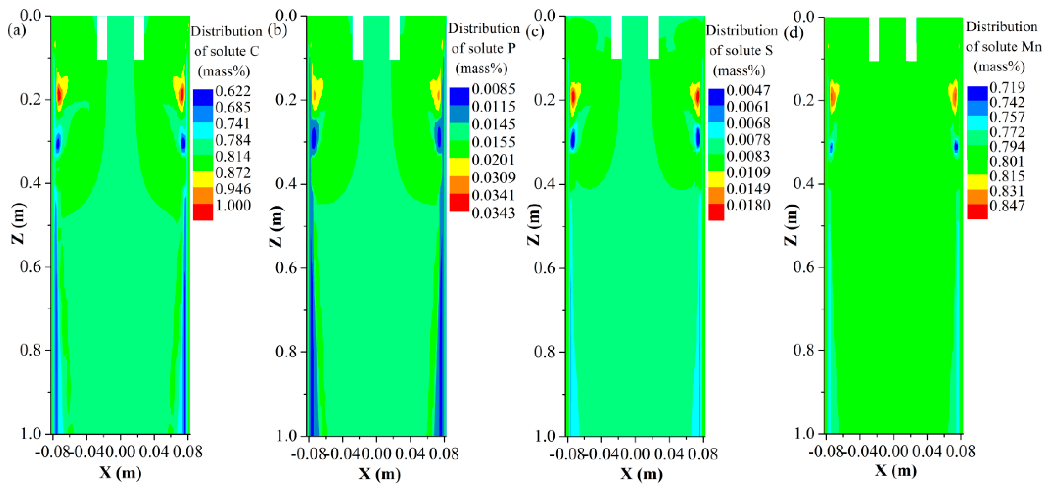
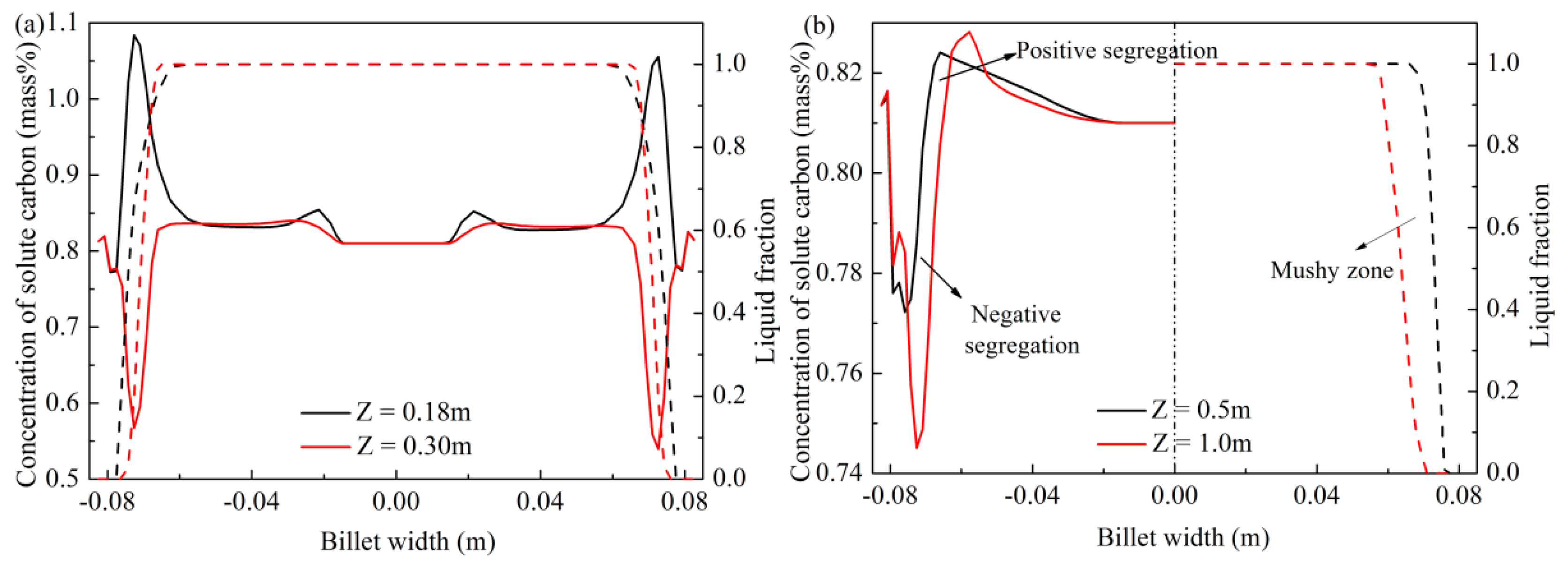
As convection, diffusion, and solidification progressed, there was measurable inhomogeneity in the solute distribution in the mold mainly occurring as solute enrichment at the upper region and negative segregation in the solidified shell. The distribution of different solute elements was predicted to be qualitatively similar.

(4)

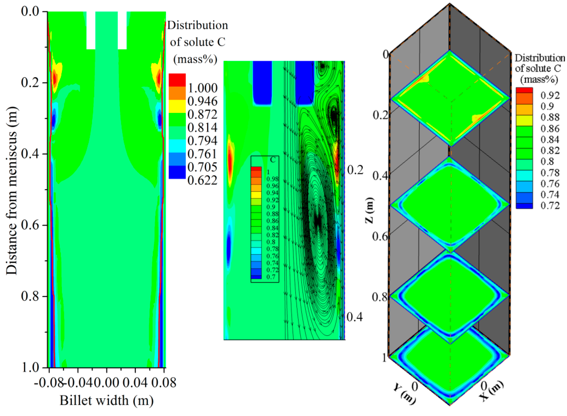
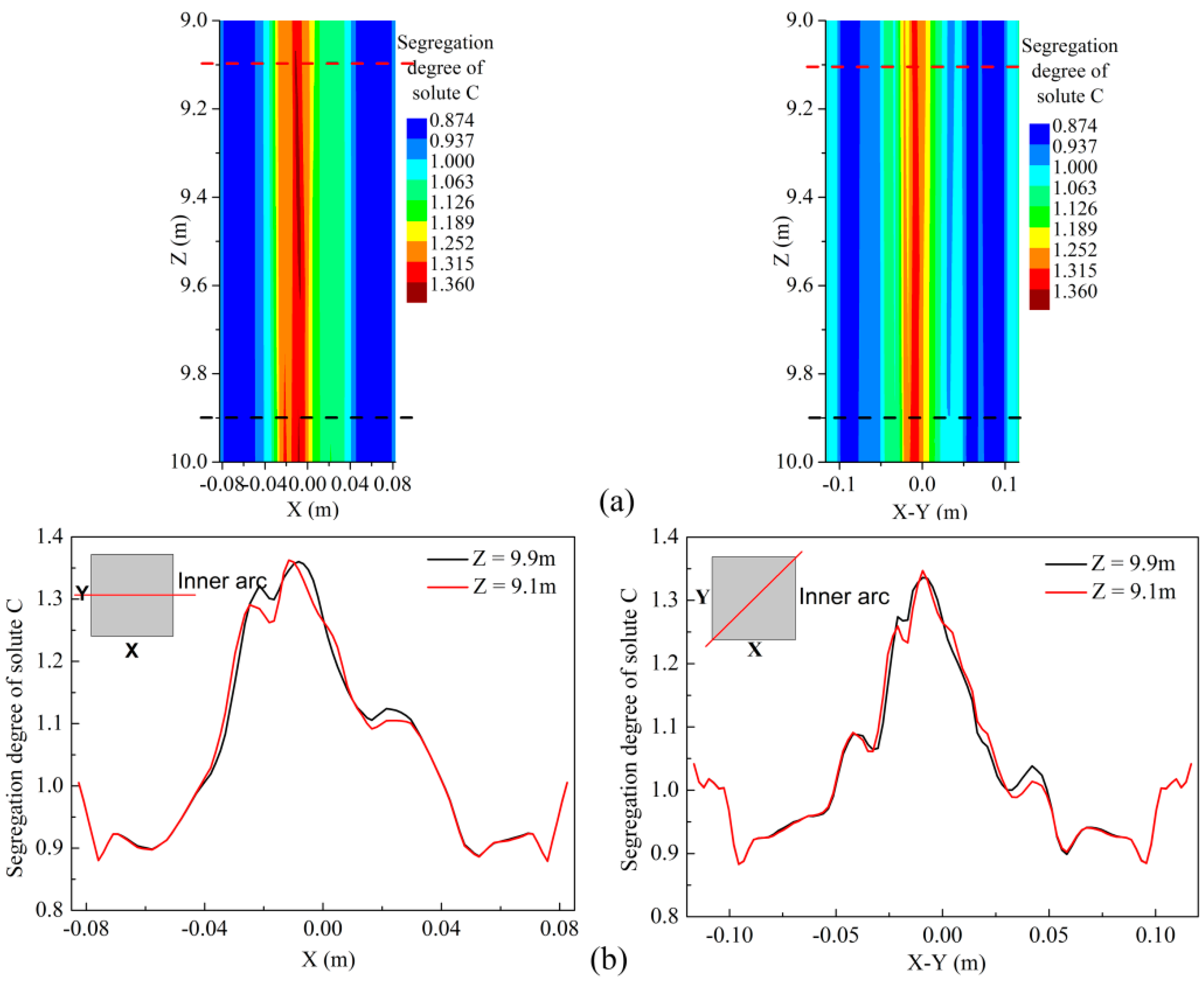
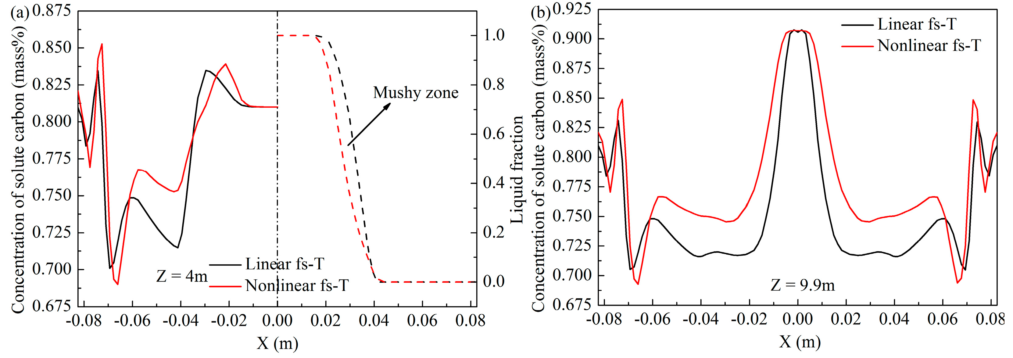
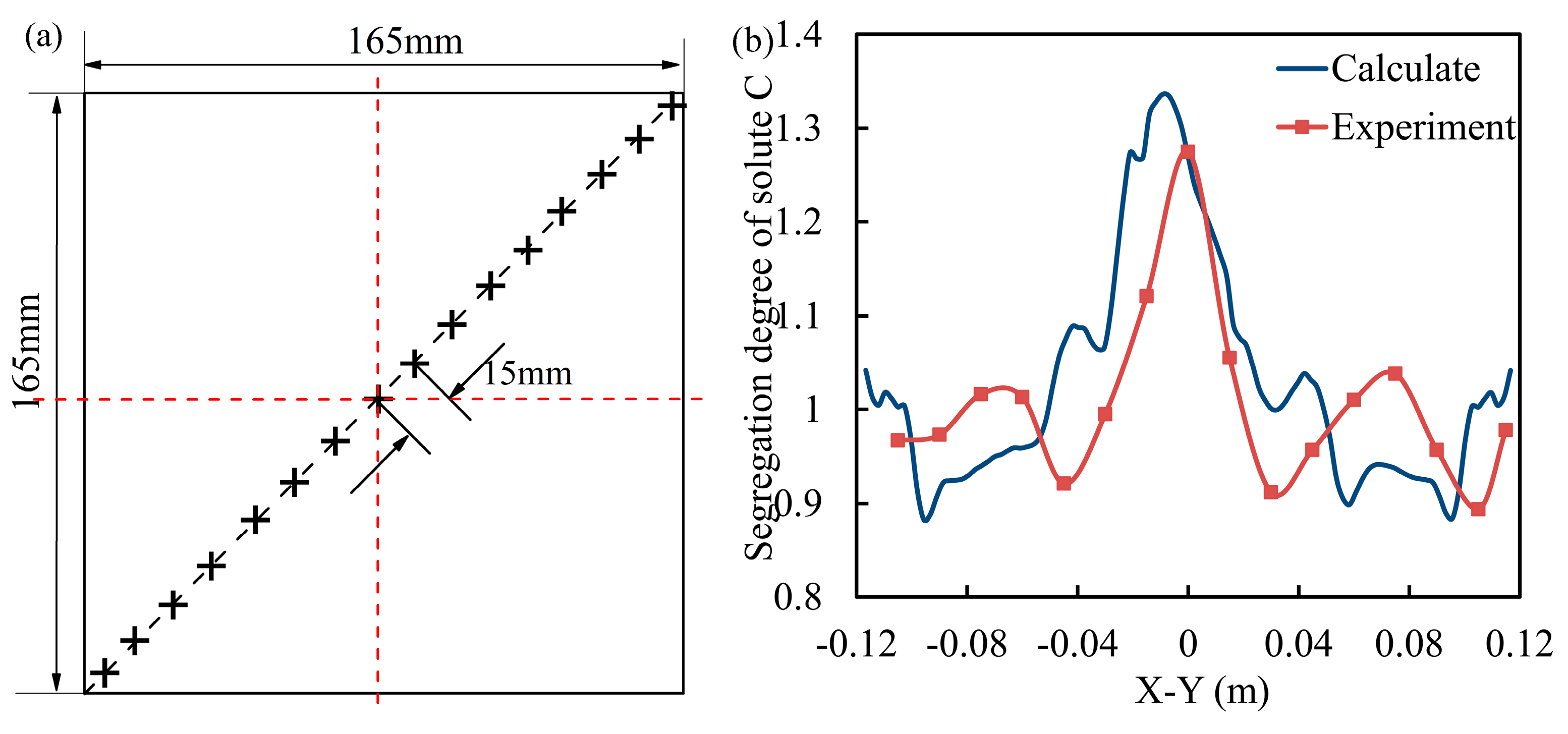
The results also suggest that the final macrosegregation patterns in the billet formed in the mushy zone with relatively low central liquid fraction, but not at the end of solidification. The segregation profiles of solute C, arising with a positively segregated peak at the centerline and a negatively segregated minima at the sides, were predicted to be similar at the longitudinal and diagonal sections. There was close agreement between the measured and calculated segregation degrees, which supports the validity of the proposed 3D macrosegregation model.

(5)

The predicted ring-shaped negative segregation zone that formed in the mold still existed at the end of solidification due to the limited solute diffusion coefficient in solid. The solute redistribution occurring at the solidification front created solute-enriched liquid near the solidified shell, which contributed to the evolution of macrosegregation alongside thermosolutal convection.

(6)

The equilibrium partition coefficient was the main contributor to the distinctions in the magnitude of macrosegregation. Comparison between solutes P and S indicated that diffusion coefficients also have a certain influence on macrosegregation.

References

1. Moon, C.H.; Oh, K.S.; Lee, J.D.; Lee, S.J.; Lee, Y. Effect of the roll surface profile on centerline segregation in soft reduction process. ISIJ Int. 2012, 52, 1266–1272. [Google Scholar] [CrossRef]
2. Sang, B.; Kang, X.; Li, D. A novel technique for reducing macrosegregation in heavy steel ingots. J. Mater. Process. Technol. 2010, 210, 703–711. [Google Scholar] [CrossRef]
3. Flemings, M.C.; Nereo, G.E. Macrosegregation. PT. 1. AIME Met. Soc. Trans. 1967, 239, 1449–1461. [Google Scholar]
4. Mehrabian, R.; Keane, M.; Flemings, M.C. Interdendritic fluid flow and macrosegregation; influence of gravity. Metall. Mater. Trans. 1970, 1, 1209–1220. [Google Scholar] [CrossRef]
5. Fujii, T.; Poirier, D.R.; Flemings, M.C. Macrosegregation in a multicomponent low alloy steel. Metall. Mater. Trans. B 1979, 10, 331–339. [Google Scholar] [CrossRef]
6. Bennon, W.D.; Incropera, F.P. A continuum model for momentum, heat and species transport in binary solid-liquid phase change systems—I. Model formulation. Int. J. Heat Mass Transf. 1987, 30, 2161–2170. [Google Scholar] [CrossRef]
7. Poole, G.M.; Heyen, M.; Nastac, L.; El-Kaddah, N. Numerical modeling of macrosegregation in binary alloys solidifying in the presence of electromagnetic stirring. Metall. Mater. Trans. B 2014, 45, 1834–1841. [Google Scholar] [CrossRef]
8. Ni, J.; Beckermann, C. A volume-averaged two-phase model for transport phenomena during solidification. Metall. Trans. B 1991, 22, 349–361. [Google Scholar] [CrossRef]
9. Zhao, X.K.; Zhang, J.M.; Lei, S.W.; Wang, Y.N. The position study of heavy reduction process for improving centerline segregation or porosity with extra-thickness slabs. Steel Res. Int. 2014, 85, 645–658. [Google Scholar] [CrossRef]
10. Li, W.S.; Shen, H.F.; Zhang, X.; Liu, B.C. Modeling of species transport and macrosegregation in heavy steel ingots. Metall. Mater. Trans. B 2014, 45, 464–471. [Google Scholar] [CrossRef]
11. Koshikawa, T.; Bellet, M.; Gandin, C.A.; Yamamura, H.; Bobadilla, M. Experimental study and two-phase numerical modeling of macrosegregation induced by solid deformation during punch pressing of solidifying steel ingots. Acta Mater. 2017, 124, 513–527. [Google Scholar] [CrossRef]
12. Wu, M.H.; Ludwig, A. A three-phase model for mixed columnar-equiaxed solidification. Metall. Mater. Trans. A 2006, 37, 1613–1631. [Google Scholar] [CrossRef]
13. Ge, H.H.; Li, J.; Han, X.J.; Xia, M.X.; Li, J.G. Dendritic model for macrosegregation prediction of large scale castings. J. Mater. Process. Technol. 2016, 227, 308–317. [Google Scholar] [CrossRef]
14. Vušanović, I.; Vertnik, R.; Šarler, B. A simple slice model for prediction of macrosegregation in continuously cast billets. IOP Conf. Ser. Mater. Sci. Eng. 2012, 27, 1–6. [Google Scholar] [CrossRef]
15. Sun, H.B.; Zhang, J.Q. Study on the macrosegregation behavior for the bloom continuous casting: Model development and validation. Metall. Mater. Trans. B 2014, 45, 1133–1149. [Google Scholar] [CrossRef]
16. Yang, H.L.; Zhang, X.Z.; Deng, K.W.; Li, W.C.; Gan, Y.; Zhao, L.G. Mathematical simulation on coupled flow, heat, and solute transport in slab continuous casting process. Metall. Mater. Trans. B 1998, 29, 1345–1356. [Google Scholar] [CrossRef]
17. Fang, Q.; Ni, H.W.; Wang, B.; Zhang, H.; Ye, F. Effects of EMS induced flow on solidification and solute transport in bloom mold. Metals 2017, 7, 72. [Google Scholar] [CrossRef]
18. Voller, V.R.; Beckermann, C. A unified model of microsegregation and coarsening. Metall. Mater. Trans. A 1999, 30, 2183–2189. [Google Scholar] [CrossRef]
19. Domitner, J.; Wu, M.H.; Kharicha, A.; Ludwig, A.; Kaufmann, B.; Reiter, J. Modeling the effects of strand surface bulging and mechanical soft reduction on the macrosegregation formation in steel continuous casting. Metall. Mater. Trans. A 2014, 45, 1415–1434. [Google Scholar] [CrossRef]
20. Won, Y.M.; Thomas, B.G. Simple model of microsegregation during solidification of steels. Metall. Mater. Trans. A 2001, 32, 1755–1767. [Google Scholar] [CrossRef]
21. Prescott, P.J.; Incropera, F.P. The effect of turbulence on solidification of a binary metal alloy with electromagnetic stirring. J. Heat Transf. 1995, 117, 716–724. [Google Scholar] [CrossRef]
22. Mathur, A.; He, S. Performance and implementation of the Launder–Sharma low-Reynolds number turbulence model. Comput. Fluids 2013, 79, 134–139. [Google Scholar] [CrossRef]
23. Schneider, M.C.; Beckermann, C. A numerical study of the combined effects of microsegregation, mushy zone permeability and flow, caused by volume contraction and thermosolutal convection, on macrosegregation and eutectic formation in binary alloy solidification. Int. J. Heat Mass Transf. 1995, 38, 3455–3473. [Google Scholar] [CrossRef]
24. Dong, Q.P.; Zhang, J.M.; Qian, L.; Yin, Y.B. Numerical modeling of macrosegregation in round billet with different microsegregation models. ISIJ Int. 2017, 57, 814–823. [Google Scholar] [CrossRef]
25. Kang, K.G.; Ryou, H.S. Computation of solidification and melting using the PISO algorithm. Numer. Heat Transf. Part B Fund. 2010, 46, 179–194. [Google Scholar] [CrossRef]
26. Du, P.F. Numerical Modeling of Porosity and Macrosegregation in Continuous Casting of Steel. Ph.D. Thesis, University of Iowa, Iowa City, IA, USA, 2013. [Google Scholar]
27. Lai, K.Y.M.; Salcudean, M.; Tanaka, S.; Guthrie, R.I.L. Mathematical modeling of flows in large tundish systems in steelmaking. Metall. Mater. Trans. B 1986, 17, 449–459. [Google Scholar] [CrossRef]
28. Chaudhuri, S.; Singh, R.K.; Patwari, K.; Majumdar, S.; Ray, A.K.; Singh, A.K.P.; Neogi, N. Design and implementation of an automated secondary cooling system for the continuous casting of billets. ISA Trans. 2010, 49, 121–129. [Google Scholar] [CrossRef] [PubMed]
29. Cao, Y.F.; Chen, Y.; Li, D.Z.; Liu, H.W.; Fu, P.X. Comparison of channel segregation formation in model alloys and steels via numerical simulations. Metall. Mater. Trans. A 2016, 47, 2927–2939. [Google Scholar] [CrossRef]
30. Ludwig, A.; Wu, M.H.; Kharicha, A. On macrosegregation. Metall. Mater. Trans. A 2015, 46, 4854–4867. [Google Scholar] [CrossRef]
31. Clyne, T.W.; Kurz, W. Solute redistribution during solidification with rapid solid state diffusion. Metall. Mater. Trans. A 1981, 12, 965–971. [Google Scholar] [CrossRef]
Figure 1. Vertical mesh adopted here (a); and reconstruction of gravitational acceleration (b).
Metals 07 00209 g001
Figure 2. Streamline distribution and velocity contour in the mold.
Metals 07 00209 g002
Figure 3. Evolution of solidification profiles along the casting direction.
Metals 07 00209 g003
Figure 4. Contour plots of liquid fraction at different sections.
Metals 07 00209 g004
Figure 5. Predicted liquid fraction profiles at different cross sections.
Metals 07 00209 g005
Figure 6. Contour plots of velocity and liquid fraction at different cross sections.
Metals 07 00209 g006
Figure 7. Distribution of different solute elements in the mold: (a) C; (b) P; (c) S; and (d) Mn.
Metals 07 00209 g007
Figure 8. Detailed distribution of solute C in the mold.
Metals 07 00209 g008
Figure 9. Predicted profiles for the concentration of solute C and liquid fraction: (a) Z = 0.18 and 0.30 m; and (b) Z = 0.5 and 1.0 m.
Metals 07 00209 g009
Figure 10. Segregation degree of solute C near the end of solidification: (a) contour plots; and (b) segregation profiles.
Metals 07 00209 g010
Figure 11. Comparison between the results calculated with linear and nonlinear fs-T functions: (a) Z = 4 m; and (b) Z = 9.9 m.
Metals 07 00209 g011
Figure 12. Validation of the model: (a) sampling scheme in experimental billet; and (b) comparison between the calculated and experimental segregation degree.
Metals 07 00209 g012
Figure 13. Computed distribution of solute C at different billet cross sections.
Metals 07 00209 g013
Figure 14. Comparison in the segregation profiles between different elements: (a) solutes C and Mn; and (b) solutes P and S.
Metals 07 00209 g014
Figure 15. Diffusion coefficients in both the liquid and solid for the solutes P and S: (a) solid zone; and (b) liquid zone.
Metals 07 00209 g015