Models to Predict the Viscosity of Metal Injection Molding Feedstock Materials as Function of Their Formulation

Abstract

The viscosity of feedstock materials is directly related to its processability during injection molding; therefore, being able to predict the viscosity of feedstock materials based on the individual properties of their components can greatly facilitate the formulation of these materials to tailor properties to improve their processability. Many empirical and semi-empirical models are available in the literature that can be used to predict the viscosity of polymeric blends and concentrated suspensions as a function of their formulation; these models can partly be used also for metal injection molding binders and feedstock materials. Among all available models, we made a narrow selection and used only simple models that do not require knowledge of molecular weight or density and have parameters with physical background. In this paper, we investigated the applicability of several of these models for two types of feedstock materials each one with different binder composition and powder loading. For each material, an optimal model was found, but each model was different; therefore, there is not a universal model that fits both materials investigated, which puts under question the underlying physical meaning of these models.

1. Introduction

Metal injection molding (MIM) is a complex, multi-step process with a significant technological and economic potential. To achieve parts with good quality, every step of the MIM process has to deliver good quality. Defects introduced in one step usually cannot be corrected in the follow-up steps. From the rheological point of view, feedstock materials for MIM can be considered as concentrated suspensions. A suspension is a complex fluid in which solid particles are suspended in a liquid continuous phase. In the case of MIM feedstocks, the liquid continuous phase is referred to as the binder system. The binder system plays a big role in the production of MIM parts, even though it is completely absent in the final part. Usually a binder system consists of different types of polymers, waxes and additives to cover all the functions a binder system has to fulfill. One of its main functions is to provide moldability to the metal powder. Here one of the main properties is viscosity and being able to predict the viscosity of feedstock materials based on the viscosities of binders and powder characteristics can greatly speed up the development of new feedstock materials for different applications.

The viscosity of the MIM feedstock materials depends among other things on the binder composition, as well as on the amount, size and shape of the metal particles. In this paper, different empirical models were investigated first to predict the binder viscosity from the known viscosity of its individual components. Then simple semi-empirical models were used to describe the viscosity of the feedstocks with different powder loadings at a fixed shear rate. The models investigated can be used to optimize the formulation of binders and feedstock materials; for example to choose the components of the binder system or the amount of powder that can be added in order to have a feedstock material with the appropriate viscosity. It is important to mention that the chosen models do not take directly into account the effects of shear rate, temperature and pressure on the viscosity of the binders nor feedstock materials; and therefore cannot be used for injection molding simulations alone. This is out of the scope of this paper.

In summary, this paper has three main goals: First to evaluate which existing model best describes the viscosity of multicomponent binder systems by knowing the amount of each component and the viscosity of each component at fixed boundary conditions; second, to evaluate which model from the literature best describes the viscosity of feedstock materials by knowing the viscosity of the binder system at fixed boundary conditions and the amount of powder present in the feedstock; and third, to determine if there is a universal model that can be applied to a different binders and feedstocks. In order to test this last hypothesis, two very distinct binders with different chemical composition and two feedstocks with different binders and different particle size distribution were selected. The paper does not try to draw conclusions on the effect of different binder systems and particle size distribution on the viscosity of feedstocks, but rather to give examples of very different binders and feedstock materials.

2. Theoretical Background

2.1. Models for Viscosity Prediction of Multicomponent Binders

Multicomponent binders for MIM are polymeric blends and additives made to fulfil the requirements needed at different steps of the MIM process. Properties of blends are intermediate between those of the individual components in the blend; this is also known as additive behavior. Such additive behavior is often referred to as the “rule of mixtures”. Deviations from this rule reflect synergistic effects of mixing. Ideally, mixing two constituents enhance a material’s property beyond simple additivity; thereby exhibiting synergistic behavior [1]. Synergistic effects have been observed for example in nanocomposites where adding a small amount of nanoparticles leads to a substantial increase in their mechanical and barrier properties [2], as well as their thermal conductivity [3].

The rule of mixtures can be used for any physical property of multiphase systems such as composites and blends; this of course includes viscosity [4]. There exist numerous models for viscosities of mixtures and this paper does not intend to present all of them, but rather just a narrow selection of representative models. For a more detailed literature review on the rule of mixtures, the reader is referred to the works of Viswanath et al. [5], Centeno et al. [6] and Tariq et al. [7].

Selected models for predicting viscosity of binary mixtures and their equations are given in

Table 1. Selected viscosity models for binary mixtures.

Author(s)	Year	Equation of the Model *	Equation Number
Arrhenius [8]	1887	${\text{log}\mathsf{\eta }}_m=w_1{\text{log}\mathsf{\eta }}_1+w_2{\text{log}\mathsf{\eta }}_2$	(1)
Voigt [9]	1889	${\mathsf{\eta }}_m=w_1{\mathsf{\eta }}_1+w_2{\mathsf{\eta }}_2$	(2)
Bingham [10]	1911	$\frac{1}{{\mathsf{\eta }}_m}=\frac{w_1}{{\mathsf{\eta }}_1}+\frac{w_2}{{\mathsf{\eta }}_2}$	(3)
Van Der Wyk [11]	1936	${\text{ln}\mathsf{\eta }}_m=x_1^2\text{ln}\left(\frac{{\mathsf{\eta }}_1{\mathsf{\eta }}_2}{{\mathsf{\eta }}_{12}{}^2}\right)+2x_1\text{ln}\left(\frac{{\mathsf{\eta }}_{12}}{{\mathsf{\eta }}_2}\right)+{\text{ln}\mathsf{\eta }}_2$	(4)
Grunberg and Nissan ** [12]	1946	${\text{log}\mathsf{\eta }}_m=w_1{\text{log}\mathsf{\eta }}_1+w_2{\text{log}\mathsf{\eta }}_2+w_1{w}_2\text{log}d$	(5)
Tamura and Kurata [13]	1952	${\text{ln}\mathsf{\eta }}_m=x_1{\mathsf{\eta }}_1{\mathsf{\phi }}_1+x_1{\mathsf{\eta }}_1{\mathsf{\phi }}_1+x_2{\mathsf{\eta }}_2{\mathsf{\phi }}_2+2{\mathsf{\eta }}_{12}\sqrt{x_1{x}_2{\mathsf{\phi }}_1{\mathsf{\phi }}_2}$	(6)
Lima [14]	1952	$\text{log}(\text{log }{\mathsf{\eta }}_m)={\mathsf{\rho }}_m\left[\frac{\left(x_1{I}_1+x_2{I}_2\right)}{\left(x_1{M}_1+x_2{M}_2\right)}\right]-2.9$	(7)
McAllister [15]	1960	${\text{ln}\mathsf{\eta }}_m=x_1{}^3{\text{ln}\mathsf{\eta }}_1+3x_1{}^2{\text{ln}\mathsf{\eta }}_{12}+3x_1{\text{ln}\mathsf{\eta }}_{21}+x_2{}^3{\text{ln}\mathsf{\eta }}_2-\ln \left(x_1+x_2\frac{M_1}{M_2}\right)+3x_1{}^2{x}_2\ln \left(\frac{2+\frac{M_2}{M_1}}{3}\right)+3x_1{x}_2{}^2\text{ln}\left(\frac{1+\frac{M_2}{M_1}}{3}\right)+x_2{}^3\text{ln}\frac{M_2}{M_1}$	(8)
Heric [16]	1966	${\mathsf{\eta }}_m=\frac{{\left(M_1{\mathsf{\eta }}_1\right)}^{x_1}{\left(M_2{\mathsf{\eta }}_2\right)}^{x_2}}{M}$	(9)

* where ${\mathsf{\eta }}_m$—viscosity of the mixture; ${\mathsf{\eta }}_i{\mathsf{\eta }}_1{\mathsf{\eta }}_2$—viscosities of the components; $w_i{w}_1{w}_2$—weight fractions of the components; $x_i{x}_1{x}_2$—mole fractions of the components; ${\mathsf{\phi }}_1{\mathsf{\phi }}_2$—volume fractions of the components; d and ${\mathsf{\eta }}_{12}$—interaction parameters; ${\mathsf{\rho }}_m$—density of mixture; $I_1{I}_2$—viscosities constants of the components; $M_1{M}_2$—molecular weights of the components. ** version shown here is the one suggested by Kukla et al. [17] in which the logarithm of interaction parameter $d$ is used instead of just $d$.

. Please note that mixing rules can also be extended beyond binary mixtures, but for simplicity and because of the blends investigated, binary mixing rules are shown here. In Table 1, Equations (1) and (2) are simple models that depend on the viscosity and weight fraction of each component; these models neglect interactions between the different components of the mixture. Equations (3)–(5) take the influence of interactions into account. Finally, Equations (6)–(9) are not only based on the viscosity of each component and the related weight fractions but additionally introduce molecular weight and density as influencing factors.

As can be seen in Table 1, there is a long history on the prediction of physical properties using rule of mixtures. The first equation in Table 1 was proposed in 1887 and the last one in 1966. However in this work, we only compare the experimental data to the prediction of models that require only viscosities of individual components, their weight proportion in the mixture and maximum one fitting parameter (i.e., Equations (1)–(5)). This was done because in many occasions the molecular weight and the density at the measured temperature are not easily obtainable for each of the components. Therefore, models described by Equations (6)–(9) are less practical. Consequently, for this investigation five different models were selected: Arrhenius [8], Voigt [9], Bingham [10], van der Wyk [11], and Grunberg and Nissan [12]. The other models are shown to give examples of the level of complexity that can be used to predict the viscosity of blends, for example the model proposed by McAllister [15] has 8 different groups of factors that are being added together.

The mixing rules proposed by Arrhenius, Voigt, and Bingham are sometimes referred to as pure mixing rules. They are easy to apply, as they require viscosities of components and compositions of mixtures in terms of volume or weight fractions. On the other hand, mixing rules proposed by Van der Wyk and Grunberg and Nissan require knowledge of the viscosity of the components and their volume or weight fractions, as well as a binary interaction parameter that can be obtained by mathematical methods. In our case, the interaction parameters were obtained by using the nonlinear generalized reduced gradient algorithm [18] by minimizing the sum of square differences.

2.2. Models for Viscosity Prediction of Feedstocks with Different Filler Contents

In the literature a great number of models are available to describe the dependence of the viscosity on the volume concentration of fillers in a suspension ($\mathsf{\varphi }$). In all these models the suspension’s viscosity ($\mathsf{\eta }$) is normalized by the viscosity of the suspending fluid (${\mathsf{\eta }}_0$); therefore the term relative viscosity is introduced (${\mathsf{\eta }}_r=\mathsf{\eta }/{\mathsf{\eta }}_0$). Einstein was the first to address the suspension behavior in the dilute limit theoretically ([19], corrected [20]). He derived an analytical solution for the hydrodynamics around an isolated sphere which yields [21]:

$${\mathsf{\eta }}_r=1+B·\mathsf{\varphi }$$

(10)

where the constant $B$ is variously referred to as the Einstein coefficient or the intrinsic viscosity, and it takes the value $B$ = 2.5 for rigid spheres [21].

It has been observed that the viscosity of concentrated suspensions, including MIM feedstocks, increases rapidly and non-linearly as the solid content increases up to the point where the viscosity is infinite [22,23]. Therefore, the model proposed by Einstein is not able to correctly describe the viscosity of concentrated suspensions ($\mathsf{\varphi }$ > 0.2). For this reason, further models have been developed, which include the limiting parameter known as the maximum packing fraction or critical volume fraction (${\mathsf{\varphi }}_m$). The maximum packing fraction represents the solid content at which the viscosity of a concentrated suspension becomes infinite.

The models in the literature can be structured into two groups [24]: Exponential models (Mooney type) and Power-law models (Krieger type).

Table 2. Selected models to predict the relative viscosity (${\mathsf{\eta }}_r$) of concentrated suspensions as a function of filler content ($\mathsf{\varphi }$) and maximum packing fraction (${\mathsf{\varphi }}_m$). Please note that B is the intrinsic viscosity like in the Einstein’s equation.

Model Author(s)	Year	Equation of the Model	Equation Number
Eilers [25]	1941	${\mathsf{\eta }}_r={\left(1+\frac{1}{2}B\left(\frac{\left(\frac{\mathsf{\varphi }}{{\mathsf{\varphi }}_m}\right)}{1-\left(\frac{\mathsf{\varphi }}{{\mathsf{\varphi }}_m}\right)}\right)\right)}^2$	(11)
Mooney [26]	1951	${\mathsf{\eta }}_r=e^{\left(\frac{B\mathsf{\varphi }}{1-\frac{\mathsf{\varphi }}{{\mathsf{\varphi }}_m}}\right)}$	(12)
Krieger and Dougherty [27]	1959	${\mathsf{\eta }}_r={\left(1-\frac{\mathsf{\varphi }}{{\mathsf{\varphi }}_m}\right)}^{-B{\mathsf{\varphi }}_m}$	(13)
Frankel and Acrivos [28]	1967	${\mathsf{\eta }}_r=\frac{9}{8}\left(\frac{{\left(\frac{\mathsf{\varphi }}{{\mathsf{\varphi }}_m}\right)}^{\frac{1}{3}}}{1-{\left(\frac{\mathsf{\varphi }}{{\mathsf{\varphi }}_m}\right)}^{\frac{1}{3}}}\right)$	(14)
Chong et al. [22]	1971	${\mathsf{\eta }}_r={\left(1+0.75\left(\frac{\left(\frac{\mathsf{\varphi }}{{\mathsf{\varphi }}_m}\right)}{1-\left(\frac{\mathsf{\varphi }}{{\mathsf{\varphi }}_m}\right)}\right)\right)}^2$	(15)
Quemada [29]	1977	${\mathsf{\eta }}_r={\left(1-\frac{\mathsf{\varphi }}{{\mathsf{\varphi }}_m}\right)}^{-2}$	(16)
Van den Brule and Jongschaap [30]	1991	${\mathsf{\eta }}_r=1+\frac{9}{8}{\mathsf{\varphi }}_m\left(\frac{{\left(\frac{\mathsf{\varphi }}{{\mathsf{\varphi }}_m}\right)}^{\frac{1}{3}}}{1-{\left(\frac{\mathsf{\varphi }}{{\mathsf{\varphi }}_m}\right)}^{\frac{1}{3}}}\right)$	(17)
Janardhana et al. [31]	2000	${\mathsf{\eta }}_r={\left(1-\frac{\mathsf{\varphi }}{{\mathsf{\varphi }}_m}\right)}^{-1}$	(18)
Zarraga et al. [32]	2000	${\mathsf{\eta }}_r=e^{-2.34\mathsf{\varphi }}{\left(1-\frac{\mathsf{\varphi }}{{\mathsf{\varphi }}_m}\right)}^{-3}$	(19)
Mendoza and Santamaria-Holek [33]	2009	${\mathsf{\eta }}_r={\left(1-\frac{\mathsf{\varphi }}{1-\mathsf{\varphi }c}\right)}^{-2.5}$ $c=\frac{1-{\mathsf{\varphi }}_m}{{\mathsf{\varphi }}_m}$	(20)
Pal [34]	2015	${\mathsf{\eta }}_r=e^{\left(\frac{\left(2.5\left(\frac{n+1}{2}\right)+\left(\frac{n-1}{2}\right)\right)\mathsf{\varphi }}{1-\frac{\mathsf{\varphi }}{{\mathsf{\varphi }}_m}}\right)}$	(21)

shows 3 exponential and 9 power law models found in the literature in chronological order [22,25,26,27,28,29,30,31,32,33,34].

In this investigation, only models for high solid content and with one fitting parameter (i.e., ${\mathsf{\varphi }}_m$) were used. These models are relatively simple since they only require viscosity measurements and eliminate fitting of parameters that may not have an actual physical meaning or would require additional measurements. The model suggested by Pal [34] was also not used since it assumes that the viscosity of the fluid phase can be modelled by a power law where $n$ is the power-law index, and as it will be shown in the results, that was not necessarily the case for the binder systems at the shear rates investigated here.

Therefore, the models investigated included the ones proposed by Frankel and Acrivos [28]; Chong et al. [22]; Quemada [29]; van den Brule and Jongschaap [30]; Janardhana et al. [30]; Zarraga et al. [32]; and Mendoza and Santamaria-Holek [33]. In the next paragraphs a brief description of these models is provided.

Frankel and Acrivos treated solid spheres as fluid elements with regard to their instantaneous motion and investigated the hydrodynamic interactions between particles in relative motion. They equate the ratio between the energy dissipation in the suspension and in the homogeneous fluid to the relative viscosity of the suspension. The constant 9/8 comes from the spherical cell model in a cubic configuration of neighboring particles chosen for determination of velocity field [28].

The empirical equation proposed by Chong et al. was estimated by fitting extensive data from their experiments on monomodal and bimodal glass bead suspensions and the available literature at that time. They modified the Eilers’ equation with a constant coefficient of 0.75. For uniform-size spherical particles at dilute concentrations the Chong et al. equation reduces to the Einstein’s equation (assuming ${\mathsf{\varphi }}_m$ = 0.605, which represents an orthorhombic packing) [22].

Quemada’s model is based on a concentrated disperse media flowing in narrow ducts where viscosity is a function of powder loading, concentration takes a rectangular profile and no effective diffusion occurs. Rectangular profile considers a no-slip condition at walls and homogeneous distribution of both phases. His model does not reduce to Einstein’s equation when applied to dilute suspensions, but it agrees with experimental data very well [29].

Van den Brule and Jongschaap used the Frankel and Acrivos principle as a starting point where they replaced energy dissipation with stress tensor of a concentrated suspension. Their theory equates the stress tensor to relative viscosity of the suspension. For determining of the stress tensor, they used local volume averaging method where it is assumed that the volume-averaged value of a certain property equals to the macroscopically observable value of the same property [30].

Janardhana et al. derived their model from a rule of mixtures similar to the Bingham model (Equation (3)) in which the fluidity ($1/\mathsf{\eta }$) of a feedstock material is the sum of fluidity of its constituents. However it assumes that the flow is only due to the binder since the powder does not flow under shear due to inter-particulate friction and that there is a critical binder content at which all liquid present in the feedstock is utilized for filling up the particle structure in close packing [31].

Zarraga et al. introduced a correlation for the relative viscosity, which obeys the Einstein’s relation in the dilute limit while diverging at maximum random close packing. This equation was obtained by fitting their viscosity data of glass bead suspensions. The equation was then implemented into equations of stress in the vorticity direction in order to calculate the normal stress difference of suspensions [32].

Mendoza and Santamaria-Holek used differential effective medium approach. The DEMT (Differential Effective Medium Theory) is based in a progressive addition of spheres to the sample. A suspension, into which a small additional quantity of particles is added, is treated as a homogeneous effective medium with correlating viscosity [33].

3. Materials and Methods

3.1. Materials

Two types of feedstock materials were prepared for this investigation. These two types of feedstocks differ in their binder composition and particle size distribution. The first feedstock had a binder composed of a mixture of polypropylenes, while the second one had a binder composed of a mixture of polyoxymethylenes. The polypropylene-based feedstock can be debound with solvents or thermally, while the polyoxymethylene-based feedstock is generally debound catalytically, but in principle thermal and solvent debinding is possible.

As mentioned in the introduction, the binder of MIM feedstock is usually composed of several components in order to adjust the flow properties of the material and to provide good mechanical properties to the green part after molding. The two binder systems presented in the paper are composed of two types of polymers that have similar chemistry but different mechanical and flow properties. The polypropylene (PP) binder system is composed of PP and PP-wax. A wax is a low molecular weight version of a polymer and it is usually added to the binder to reduce its viscosity. On the other hand, the polyoxymethylene (POM) binder system is composed of a high molecular weight POM that provides strength to the molded part and a low molecular weight POM that increases the flowability of the binder system when molding.

Both types of feedstock contained 316L stainless steel particles with spherical shape, but different particle size distributions. Feedstock materials with different powder content were investigated. The characterization of feedstock materials with different powder content is used to estimate the maximum amount of powder that can be added to a feedstock material without increasing the viscosity beyond processable values ($\mathsf{\varphi }<{\mathsf{\varphi }}_m)$. Since the maximum amount of powder that can be added to a feedstock is dependent on the binder viscosity and the particle size distribution, it is hard to estimate a priori the powder content at which the particle-particle interactions become more relevant for each feedstock, so it is better to also have feedstock with low powder loading, e.g., ~20 vol. %. Additionally, the used models can be validated especially regarding applicability for different powder loadings.

3.1.1. Polypropylene-Based Feedstock

The first binder system investigated consisted of polypropylene—PP (PP HB306MO, Borealis, Vienna, Austria), polypropylene wax—wax (Licocene PP 7502, Clariant, Frankfurt am Main, Germany) and stearic acid—SA (MERCK Schuchardt OHG, Hohenbrunn, Germany).

Commercially available 316L stainless steel powder (Sandvik Osprey Ltd., Neath, UK) with particle size distribution of D10 = 4.5 μm, D50 = 13.7 μm and D90 = 31.9 μm was used to achieve feedstocks with 10, 20, 30, 40, 50, 60, 64, 68 and 72 vol. % powder loading.

The PP-based feedstocks were prepared in a laboratory kneader (Brabender Plasticorder, PL-2000, Brabender GmbH & Co. Kg., Duisburg, Germany) using counter-rotating rollers. Mixing temperature was set at 175 °C and the rotational speed at 60 rpm. During the feedstock production, a small amount of polymeric binder was pre-melted in the mixing chamber for about 3 min. Then the remaining binder and powder were added. Mixing was carried out for additional 25 min [17].

3.1.2. Polyoxymethylene-Based Feedstock

The second binder system investigated consisted of commercially available polyoxymethylene—POM1 (Ultraform^® Z2320, BASF SE, Ludwigshafen, Germany) and laboratory synthesized polyoxymethylene—POM2 (BASF SE, Ludwigshafen, Germany). The main difference of the two POM components was their molecular weight with the commercial one having a larger average molecular weight than the laboratory one. No surfactants or compatibilizers were used.

316L stainless steel powder was supplied by BASF after a process of centrifugation to obtain a customized particle size distribution (D10 = 1.35 μm, D50 = 2.74 μm and D90 = 6.80 μm). The powder was used to achieve feedstocks with 21, 24, 30, 40, 47, and 62 vol. % powder loading.

The POM-based feedstocks were prepared in a laboratory mixing extruder (Custom Scientific Instruments, Easton, PA, USA). Extrusion was performed at 190 °C. POM1, POM2 and 316L steel were in powder form. The three materials were premixed in solid state and then slowly fed into the extruder; after extrusion the extrudate was ground in a commercial coffee grinder (Braun GmbH, Kronberg im Taunus, Germany). After milling the feedstock was extruded three more times and sequentially milled 3 more times to ensure a homogeneous feedstock composition [35].

3.2. Methods

The viscosity of feedstock materials can be measured using different devices depending on the shear rates one is interested on measuring. During MIM, the shear rates experienced vary from 10² to 10⁵ s⁻¹ [36]. In order to capture this range is better to perform viscosity measurements in rotational rheometers, capillary rheometers and instrumented extruders or injection molding machines. However to obtain the full range of shear rates, large amounts of materials are needed, particularly when utilizing instrumented processing equipment. Nevertheless, measuring the viscosity in rheometers still provides a good indication if the material will have a better or worse flow behavior during injection molding.

Viscosity measurements were performed in rotational and capillary rheometers to have a broad range of shear rates without using very large amounts of materials. Unfortunately, due to the small amount of experimental POM and customized particle size distribution powder available, it was only possible to perform viscosity measurement in a rotational rheometer for feedstocks with a POM-based binder. For the PP-based feedstocks, rotational and capillary viscosity measurements were performed.

3.2.1. Rotational Rheometry

Viscosity for PP-based feedstocks was measured using a MCR501 rotational rheometer (Anton Paar GmbH, Graz, Austria) in oscillating mode with plate-plate geometry of 50 mm diameter for binder components and 25 mm diameter for feedstocks. Frequency sweeps measurements in the range from 0.1 to 500 rad/s were made at strains in the linear viscoelastic range. For feedstocks materials with powder content between 10 and 30 vol. % it was observed that the Cox-Merz rule [37] applies, for this reason only oscillatory tests were performed. For feedstocks with higher particle content than 30 vol. % only capillary rheometry was performed because these materials were prone to slip in the rotational rheometer. All of these measurements were performed at 170 °C.

Viscosity measurements for POM-based materials were performed using a MARS II rotational rheometer (Thermo Scientific, Karlsruhe, Germany) with plate-plate geometry of 20 mm diameter. For the binder components measurements were done in oscillatory mode, but for feedstock materials they were done in constant rotational mode. This was done since it was observed that for the pure binder components the Cox-Merz rule applies, but it was not the case for feedstock materials with POM binders. Oscillatory measurements were performed in the range of 0.06 to 600 rad/s with an applied stress within the linear viscoelastic region. Constant rotational measurements were done in the shear rate range from 0.1 to 100 s⁻¹. All of these measurements were performed at 180 °C.

Viscosity measurements for PP and POM were performed at different temperatures because these two polymers have different melting temperatures and also different recommended processing temperatures.

3.2.2. Capillary Rheometry

Feedstock materials are subjected to high shear rates (10²–10⁵ s⁻¹) during the injection molding process. In order to measure viscosity at these high shear rates, capillary rheometers or instrumented injection molding machines are used. Here, viscosity measurements on PP-based binder and feedstocks at shear rates from approximately 100 to approximately 4000 s⁻¹ were performed on a Rheograph 2002 high pressure capillary rheometer (Göttfert Werkstoff-Prüfmaschinen GmbH, Buchen, Germany). For PP-based binder and its components, three round capillaries with diameter of 0.5 mm and three lengths (5 mm, 10 mm and 15 mm) were used.

Flow behavior of highly-filled feedstocks (from 40 to 72 vol. %) was investigated using a high pressure capillary rheometer with a slit die with flush-mounted pressure transducers. Width of the slit was 10 mm and height of 1 mm, thus they fulfil the requirement of “infinitely wide” (w ≥ 10 h) slit. Further rheological investigations on feedstocks with 10, 20 and 30 vol. % powder loading were done using the capillary rheometer with the round die (D = 1 mm) and three lengths (5 mm, 10 mm and 15 mm).

In order to determine the true viscosity curve corrections were done. The true shear stress at round die was calculated from the Bagley correction [38]. In addition, by using the Weissenberg-Rabinowitsch equation [39] the true shear rates were obtained for the slit and round dies. These measurements were performed at 170 °C.

4. Results and Discussion

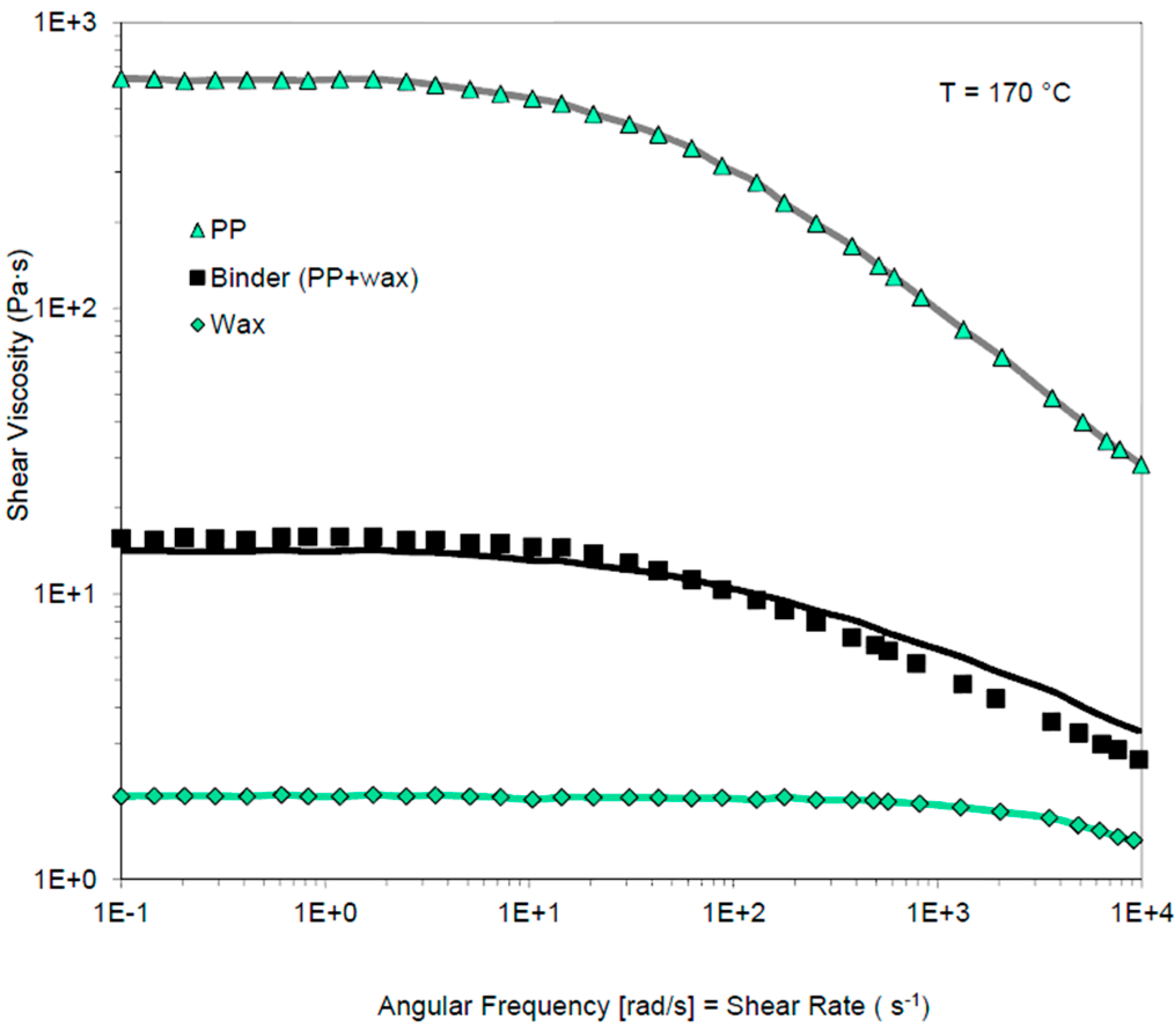
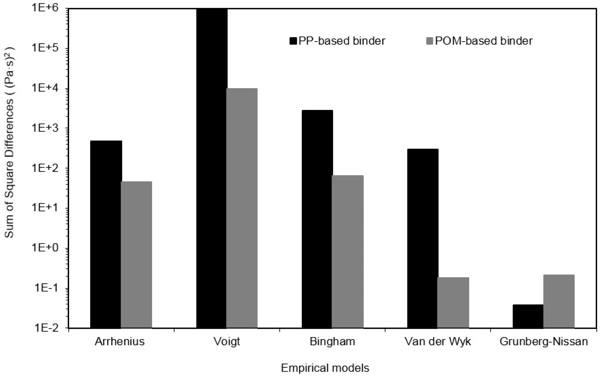
4.1. Viscosity of Binders

The viscosity of the PP-based binder and its individual components as a function of angular frequency and shear rate is shown in Figure 1. It can be seen that polypropylene (PP) has a viscosity much higher than the polypropylene wax (wax), while their mixture (Binder) lies somewhere in between them. As it was explained in the introduction, this is an example of additive behavior and thus a rule of mixtures can be applied. In Figure 1 the viscosity of PP and wax has been fitted with the Carreau model [40]:

$$\mathsf{\eta }={\mathsf{\eta }}_{\infty }+({\mathsf{\eta }}_0-{\mathsf{\eta }}_{\infty }){(1+(\mathsf{\lambda }(\dot{\mathsf{\gamma }}{)}^2)}^{\frac{\left(n-1\right)}{2}}$$

(22)

where $\dot{\mathsf{\gamma }}$ is the shear rate in s⁻¹, ${\mathsf{\eta }}_{\infty }$ is the viscosity constant at large shear rates ($\dot{\mathsf{\gamma }}\to \infty$) in Pa·s, ${\mathsf{\eta }}_0$ is the viscosity constant at low shear rates ($\dot{\mathsf{\gamma }}\to 0$) in Pa·s, $\mathsf{\lambda }$ is the relaxation time constant in s, and $n$ is the dimensionless power law index. Fitting the viscosity curve of the individual binder components to the Carreau model allows us to interpolate the viscosities at shear rates where no experimental data is available. The Carreau model can also be used to fit the viscosity curve of the binder (PP + wax) as a function of shear rate, but this is not shown in Figure 1. In Figure 1 the binder viscosity curve is fitted to the rule of mixtures that best fits the data.

The binder’s viscosities were fitted by 5 distinct mixing rules in order to find the most applicable to our multicomponent binder systems. The models investigated here included the ones proposed by Arrhenius [8]; Voigt [9]; van der Wyk [11]; and Grunberg and Nissan [12]. All the fittings were performed using the nonlinear generalized reduced gradient algorithm [18] implemented in Excel Solver by minimizing the sum of square differences between the measured viscosity and the calculated viscosity (Equation (23)).

$$S={\displaystyle \sum }_{i=1}^N{\left(M_i-C_i\right)}^2$$

(23)

where $\mathrm{S}$ is the sum of the square difference, $M_i$ is the measured viscosity at a given shear rate, $C_i$ is the calculated viscosity at a given shear rate and N is the total number of measured points.

Among the models selected in this paper (Equations (1)–(5) in Table 1), the Grunberg-Nissan model (Equation (5)) was the one that best fitted the experimental data for the PP-based binder. The comparison to other models will be shown later on.

Figure 2 shows the viscosity of the POM-based binder and its individual components as a function of angular frequency. It can be seen that POM1 has a viscosity three orders of magnitude higher than POM2. The viscosity of the POM mixture (Binder) lies between the individual components, again indicating an additive behavior of the viscosity. Since in the frequency range investigated the viscosity is independent on the frequency (i.e., Newtonian viscosity), the individual components of the binder have been fitted by their average value, which allows interpolation between experimental data points. The viscosity curve of the binder (POM1 + POM2) could also be fitted by their average value, since it is also independent of shear rate, but this is not shown in Figure 2. In Figure 2, the binder’s viscosities were fitted using the van der Wyk model, listed in Table 1, Equation (4) since this model was the best model that described the experimental data for the POM-based binder. The results from other models will be shown later on (Figure 3).

Figure 1 and Figure 2 show the prediction of the viscosities of two distinct binder systems by two distinct models. The PP-based binder system has a better fit by the Grunberg-Nissan model and thus these predictions are shown in Figure 1. The viscosities at different shear rates of the POM-based binder system are better described by the van de Wyk model and for this reason these predictions are shown in Figure 2. All rule of mixtures models rely on the experimental data for making their predictions at a given shear rate, these models cannot be used to extrapolate or even interpolate between data points, therefore if there is a discontinuity on the experimental data of one of the components of the mixture, such discontinuity will be visible in the prediction of the models.

How well a model fits the experimental data was determined by calculating the sum of the square differences between the calculated data and the measured data at a given angular frequency or shear rate. In other words, the smaller the sum of square differences the better the fit. The comparison of 5 different models (Equations (1)–(5)) for the two binder systems is shown in Figure 3. In Figure 3, it can be seen that for the PP-based binder the best fit is undeniably the Grunberg-Nissan model. However, for the POM-based binder the van der Wyk model is only marginally better to the Grunberg-Nissan model (i.e., the sum of the square differences for the van der Wyk model is 0.179 (Pa·s)² and for the Grunberg-Nissan model is 0.211 (Pa·s)²). It is important to mention that these two models include an interaction parameter. Pure mixing rules (Equations (1)–(3) in Table 1) were not so accurate in their predictions. The reason why models with an interactive parameter fit better the experimental data could be related to the miscibility of the components in the binder. Most polymeric materials are immiscible with one another, which mean that, if they are properly dispersed their properties can be estimated by simple mixing rules (Equations (1)–(3)). However when polymers with similar chemistry are mixed together (e.g., PP + PP-wax and POM1 + POM2) there could be portions that are miscible with one another, which directly interact with one another and thus an interacting parameter is needed to predict the properties of the binder. It is important to mention that miscibility is temperature dependent; therefore, it is possible that at a certain temperature the two polymers might become immiscible and simple mixing rules can be used to predict the properties of blends [42].

From this analysis, it can be concluded that depending on the composition of the binder, different mixing rules could be used to describe their viscosity in a more accurate manner. However, the Grundberg-Nissan model could provide an acceptable prediction for the two binary binder systems investigated here.

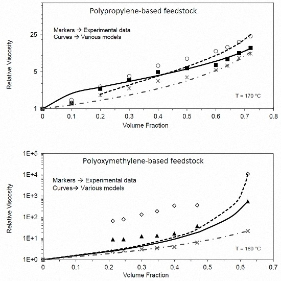
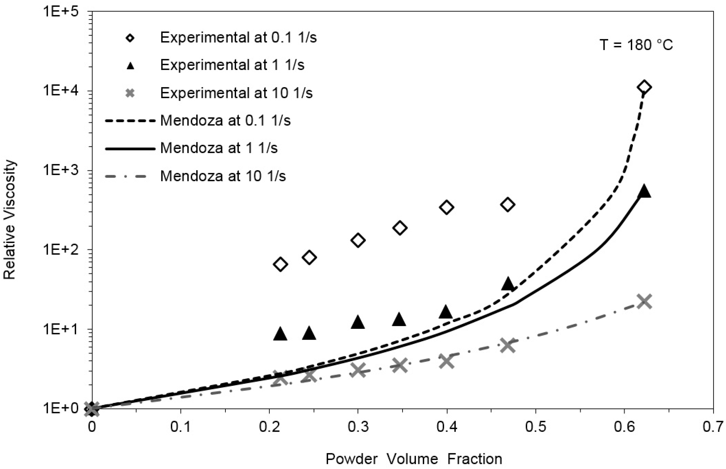
4.2. Viscosity of Feedstock Materials

The shear viscosity of MIM feedstock materials is dependent on the binder system used, the concentration of solid particles, the adherence of the binder to the powder, on the particle shape and particle size distribution. These factors not only affect the value of the viscosity, but also its dependency on shear rate (i.e., onset of shear thinning behavior) [35].

Figure 4 shows the viscosity curves for PP-based feedstock materials at different particle loadings. Lowest viscosity measure is for the pure binder system. For the binder system, the Newtonian plateau can be observed at the lowest angular frequencies (0.1 to 10 rad/s). As the powder loading increases the Newtonian plateau starts to rise and for powder loadings greater than 40 vol. %, it was not possible to measure. These viscosity data can be fitted with the Carreau model [40] (Equation (22)) and the fitting is shown by the solid lines in Figure 4.

Figure 5 shows the viscosity curves for POM-based feedstock materials at different particle loadings. It can be seen that by the addition of stainless steel powder ($\mathsf{\varphi }\to 0.2$), the rheological behavior changes from Newtonian to strong shear thinning. With higher powder content, the shear thinning becomes more pronounced and the Newtonian plateau was not accessible. The lack of Newtonian plateau in all POM-filled systems and some PP-filled ($\mathsf{\varphi }>0.3$) systems indicates the possible presence of a yield stress. The viscosity curves for POM-based feedstocks are shown up to shear rates of 10 s⁻¹ because after this shear rate, flow instabilities such as melt fracture and sample expulsion were observed.

The results of relative viscosity as a function of powder content are shown in Figure 6 and Figure 7. Both figures show that as the powder content increases the viscosity increases in a non-linear manner for the two feedstock materials at the selected shear rates: 10, 100 and 1000 s⁻¹ in Figure 6 and 0.1, 1, and 10 s⁻¹ in Figure 7. Please note that the vertical axis in Figure 6 and Figure 7 are in the logarithmic scale since by plotting the data in this way one can estimate visually if a power or exponential model will fit better the data.

In this investigation, seven distinct models were compared to find the most applicable to our MIM feedstocks. The models here investigated included the ones proposed by Frankel and Acrivos [28]; Chong et al. [22]; Quemada [29]; van den Brule and Jongschaap [30]; Jonardhama et al. [31]; Zarraga et al. [32]; and, Mendoza and Santamaria-Holek [33]. See Equations (14)–(20) listed in Table 2. These models have only one fitting parameters, namely the maximum packing fraction, ${\mathsf{\varphi }}_m$. All the fittings were performed using the nonlinear generalized reduced gradient algorithm implemented in Excel Solver [18] by minimizing the sum of square differences between the measured relative viscosity and the calculated relative viscosity (Equation (23)).

The model that best describes the relative viscosity as a function of powder loading varies depending on the material and also on which shear rate the viscosity was measured. For example, the feedstock materials containing PP are better described by the Frankel and Acrivos model at 10 s⁻¹, by the van den Brule and Jongschaap model at 100 s⁻¹ and by the Chong et al. model at 1000 s⁻¹ (Figure 6).

On the other hand, the viscosity of POM-based feedstocks is best described with the Mendoza and Santamaria-Holek model at all the selected shear rates (Figure 7). However, for the POM-based feedstock, at the two lowest shear rates (0.1 and 1 s⁻¹), all the models including the one from Mendoza and Santamaria-Holek fail to predict the relative viscosity at powder loadings between 0.2 and 0.47. This could be related to the yield stress present in POM-based feedstocks, particularly at the highest concentration of powder.

The criteria used to select which model fits best the data was again the sum of the square differences between the predicted values and the measured values. As an example, Figure 8 shows the sum of the square differences for PP- and POM-based feedstock materials for the seven selected models at the shear rate of 10 s⁻¹.

Three models can be used to predict the relative viscosity of POM feedstocks in an acceptable manner, i.e., sum of the square differences is very similar: Mendoza and Santamaria-Holek, Quemada, and van den Brule and Jongschaap; with Mendoza having the smallest sum of square differences. For PP-based feedstock materials, three models might be applicable: van den Brule, and Frankel, and Mendoza, with van den Brule having the smallest sum of square differences.

As it can be seen in Figure 8, the model proposed by Mendoza and Santamaria-Holek could be a compromise if one model should be used for both materials. The model of Mendoza and Santamaria-Holek assumes that at macroscopic length and time scales the suspension can be considered a truly continuum medium. The model takes into account that there is a finite free volume accessible to particles in a suspension, and that this free volume cannot be completely filled with spheres due to geometrical restrictions, in other words there is an excluded volume. Furthermore, the model takes into account the hydrodynamic interaction between particles, which become more important as the filling fraction increases. These hydrodynamic interactions and the excluded volume are summarized in a phenomenological parameter referred as the effective viscosity, which is equal to the volumetric loading when the suspension is diluted and equal to one when the volumetric fraction is the same as the maximum packing fraction [33]. By using this parameter, the model is able to predict in an acceptable manner the viscosity of different types of suspensions. The authors of the model stated that their model is applicable at very different shear rates, but in the present case at the lowest shear rates, the model fails to correctly describe the viscosity of feedstocks; this could be attributed to the fact that feedstocks show a yield stress, which the model does not take into account.

Since the relative viscosity curves are different for the materials investigated (Figure 6 and Figure 7), it is understandable that different models fit better the data for each material at a given shear rate. For example, the curves of the PP feedstocks do not have such a high and abrupt increase in relative viscosity as compared to the POM feedstock as the powder loading approaches the highest value.

The rate of increase in viscosity as powder loading increases is a direct effect of the particle-particle and particle-binder interactions, and therefore it depends on the spatial arrangement that the particles can achieve. The spatial arrangement of powders in a suspension depends on the particle size distribution and shape of the particles, as well as on the viscosity of the binder and shear rate at which the suspension is being sheared.

One parameter that can be used to infer the spatial arrangement of particles in a suspension is the maximum packing fraction (${\mathsf{\varphi }}_m$), which is defined as the solid content in a suspension at which its viscosity is infinite. All of the models investigated here have ${\mathsf{\varphi }}_m$ in their equations. For practical applications, a larger value of ${\mathsf{\varphi }}_m$ means that larger amounts of powder can be added to a suspension before its viscosity becomes too high. The ${\mathsf{\varphi }}_m$ values for the two feedstock materials estimated at different shear rates by their best fitting models is shown in Figure 9.

As it can be seen in Figure 9, as the shear rate increases so is the maximum packing fraction, this is seen for both feedstock materials and it has also been reported in the suspension literature [43,44]. Different maximum packing fractions occur due to the different particle orientation achieved at different shear rates. As the shear rate increases the particles in a suspension align in the direction of flow and this is manifested in a shear thinning behavior; additionally, shear also aligns the polymeric chains of the binder system in the direction of flow, thus allowing the particles to come closer together [45]. When one compares the maximum packing fraction for the two different feedstocks at the same shear rate (10 s⁻¹), it is seen that POM-based feedstock has a slightly higher ${\mathsf{\varphi }}_m$. This difference can be attributed to differences in the particle size distribution and on the different viscosity of the binder systems used. For example, a broader particle size distribution (i.e., larger range of particle sizes) leads to a higher value of ${\mathsf{\varphi }}_m$ [46] and a multimodal particle size distribution leads to a higher ${\mathsf{\varphi }}_m$ compared to a monomodal distribution [22]. In addition, lower binder viscosity is related to smaller polymeric chains, which allow more space for packing particles closer together.

In Figure 9, it can also be seen that at the lowest shear rate (0.1 s⁻¹) the value of ${\mathsf{\varphi }}_m$ is 0.63, which is relatively close to the volumetric powder loading of the most concentrated POM-based feedstock ($\mathsf{\varphi }$ = 0.62); therefore it can be expected that the viscosity of a feedstock material with 0.62 powder content will be considerably larger than feedstocks with lower powder content (see Figure 7) particularly if the volumetric content ($\mathsf{\varphi }$) is so close to the maximum packing fraction (${\mathsf{\varphi }}_m$). It is important to remember that the maximum packing fraction is the powder loading at which the viscosity of a suspension approaches infinity.

5. Conclusions

The viscosity of MIM feedstock materials is an important parameter to determine the moldability of these materials. The viscosity of MIM feedstock is dependent on its formulation, in other words on the components of the binder system and the characteristics of the metal powder. Therefore, it is a very useful tool to be able to predict the viscosity of feedstock by knowing the viscosity of its binder components and the amount of powder present in the feedstock.

In this paper, it was investigated which of the existing simple mixing rules applicable to blends can be used to predict the viscosity of multicomponent binder systems. The viscosity of both binder systems investigated lies between the viscosities of their components and for this reason mixing rules are applicable. In general, it can be said that mixing rules with an interaction parameter provide a more accurate prediction. For the PP-based binder the model proposed by Grunberg and Nissan is the most accurate, but for the POM-based binder the one proposed by van der Wyk is slightly better. In short, it can be said that there is not a universal model for predicting the viscosity of all binder systems; however, the model proposed by Grunberg and Nissan provides acceptable results for the two types of binder systems investigated here.

As expected, it was observed that the viscosity of MIM feedstock materials increases rapidly and non-linearly as a function of powder content. Therefore, exponential or power models applicable to concentrated suspensions are also applicable to MIM feedstocks. The model that best describes the viscosity of feedstocks as a function of powder loading depends not only on the material but also on the shear rate at which the viscosity is measured. Therefore, it can be said there is no model that universally fits to all feedstock materials. For the two feedstock materials here examined, if one model were to be chosen for both of them, the model proposed by Mendoza and Santamaria-Holek might represent an acceptable compromise.

The information presented here could be used for other binder or feedstock materials. For example, the Grunberg and Nissan model could be used to select the amount of each component if a target viscosity is known. Similarly, the amount of powder present in a feedstock material could be selected by using the Mendoza and Santamaria-Holek model. By utilizing these models, it is expected that the number of trials required for optimizing the formulation of binder and feedstocks could be significantly reduced. However experimental trials cannot be completely skipped, particularly if the components are very different to the ones presented here, for example for non-spherical particles.

The results presented put some shade on the physical meaning of these models and calls for their further investigation.

References

1. Lazzaro, E. Contamination in Recycling Thermoplastics used for Manufacturing of Consumer Durable Products. Master’s Thesis, Swinburne University of Technology, Melbourne, Australia, November 2009. [Google Scholar]
2. Bouakaza, B.S.; Pillin, I.; Habi, A.; Grohens, Y. Synergy between fillers in organomontmorillonite/grapheme-PLA nanocomposites. Appl. Clay Sci. 2015, 116–117, 69–77. [Google Scholar] [CrossRef]
3. Noh, Y.J.; Kim, S.Y. Synergistic improvement of thermal conductivity in polymer composites filled with pitch based carbon fiber and graphene nanoplatelets. Polym. Test. 2015, 45, 132–138. [Google Scholar] [CrossRef]
4. Grizzuti, N.; Buonocore, G.; Iorio, G. Viscous behavior and mixing rules for an immiscible model polymer blend. J. Rheol. 2000, 44, 148–164. [Google Scholar] [CrossRef]
5. Viswanath, D.S.; Ghosh, T.K.; Prasad, D.H.; Dutt, N.V.K.; Rani, K.Y. Viscosity of solutions and mixtures. In Viscosity of Liquids—Theory, Estimation, Experiment, and Data, 1st ed.; Viswanath, D.S., Ghosh, T.K., Prasad, D.H., Dutt, N.V.K., Rani, K.Y., Eds.; Springer: Dordrecht, The Netherlands, 2007; pp. 407–434. [Google Scholar]
6. Centeno, G.; Sánchez-Reyna, G.; Ancheyta, J.; Muñoz, J.A.D.; Cardona, N. Testing various mixing rules for calculation of viscosity of petroleum blends. Fuel 2011, 90, 3561–3570. [Google Scholar] [CrossRef]
7. Tariq, M.; Altamash, T.; Salavera, D.; Coronas, A.; Rebelo, L.P.N.; Lopes, J.N.C. Viscosity Mixing Rules for Binary Systems Containing One Ionic Liquid. Chem. Phys. Chem. 2013, 14, 1956–1968. [Google Scholar] [CrossRef] [PubMed]
8. Arrhenius, S.A. Über die Dissociation der in Wasser gelösten Stoffe. Z. Phys. Chem. 1887, 1, 631–649. [Google Scholar] [CrossRef]
9. Voigt, W. Ueber die Beziehung zwinschen den Beiden Elasticitätsconstanten Isotroper Körpe. Ann. Phys. 1889, 274, 573–587. [Google Scholar] [CrossRef]
10. Bingham, E.C.; White, G.F. The viscosity and fluidity of emulsions, crystalline liquids and colloidal solutions. J. Am. Chem. Soc. 1911, 33, 1257–1275. [Google Scholar] [CrossRef]
11. Van der Wyk, A.J.A. The viscosity of binary mixtures. Nature 1936, 138, 845–846. [Google Scholar] [CrossRef]
12. Grunberg, L.; Nissan, A.H. Mixture law for viscosity. Nature 1949, 164, 799–800. [Google Scholar] [CrossRef] [PubMed]
13. Tamura, M.; Kurata, M. On the viscosity of a binary mixture of liquids. Bull. Chem. Soc. Jpn. 1952, 25, 32–38. [Google Scholar] [CrossRef]
14. Lima, F.W. The viscosity of binary liquid mixtures. J. Phys. Chem. 1952, 56, 1052–1054. [Google Scholar] [CrossRef]
15. McAllister, R.A. The viscosity of liquid mixtures. AlChE J. 1960, 6, 427–431. [Google Scholar] [CrossRef]
16. Heric, E.L. On the Viscosity of Ternary Mixtures. J. Chem. Eng. Data 1966, 11, 66–68. [Google Scholar] [CrossRef]
17. Kukla, C.; Duretek, I.; Holzer, C. Rheological behaviour of binder systems for PIM and mixing rules for calculation of viscosity. In Proceedings of the Euro PM2013 Congress and Exhibition, Göteborg, Sweden, 15–18 September 2013; pp. 305–310.
18. Baker, K.R. Nonlinear programming. In Optimization Modeling with Spreadsheets, 3rd ed.; John Wiley & Sons: New York, NY, USA, 2015; pp. 270–306. [Google Scholar]
19. Einstein, A. Eine neue Bestimmung der Moleküldimensionen. Ann. Phys. 1906, 324, 289–306. [Google Scholar] [CrossRef]
20. Einstein, A. Berichtigung zu meiner Arbeit: Eine neue Bestimmung der Moleküldimensionen. Ann. Phys. 1911, 339, 591–592. [Google Scholar] [CrossRef]
21. Mueller, S.; Llewellin, E.W.; Mader, H.M. The rheology of suspensions of solid particles. Proc. R. Soc. Lond. Ser. A 2010, 466, 1201–1228. [Google Scholar] [CrossRef]
22. Chong, J.S.; Christiansen, E.B.; Baer, A.D. Rheology of concentrated suspensions. J. Appl. Polym. Sci. 1971, 15, 2007–2021. [Google Scholar] [CrossRef]
23. Kate, K.H.; Enneti, R.K.; Park, S.J.; German, R.M.; Atre, S.V. Predicting powder-polymer mixture properties for PIM design. Crit. Rev. Solid State Mater. Sci. 2014, 39, 197–214. [Google Scholar] [CrossRef]
24. Pabst, W. Fundamental considerations on suspension rheology. Ceram.-Silik. 2004, 48, 6–12. Available online: http://www.ceramics-silikaty.cz/2004/pdf/2004_01_006.pdf (accessed on 7 March 2016). [Google Scholar]
25. Eilers, H. Die Viskosität von Emulsionen hochviskoser Stoffe als Funktion der Konzentration. Kolloid-Zeitschrift 1941, 97, 313–321. [Google Scholar] [CrossRef]
26. Mooney, M. The viscosity of a concentrated suspension of spherical particles. J. Colloid Sci. 1951, 6, 162–170. [Google Scholar] [CrossRef]
27. Krieger, I.M.; Dougherty, T.J. A mechanism for non-Newtonian flow in suspensions of rigid spheres. Trans. Soc. Rheol. 1959, 3, 137–152. [Google Scholar] [CrossRef]
28. Frankel, N.A.; Acrivos, A. On viscosity of a concentrated suspension of solid spheres. Chem. Eng. Sci. 1967, 22, 847–853. [Google Scholar] [CrossRef]
29. Quemada, D. Rheology of concentrated disperse systems and minimum energy-dissipation principle—1. Viscosity-concentration relationship. Rheol. Acta 1977, 16, 82–94. [Google Scholar] [CrossRef]
30. Van den Brule, B.H.A.A.; Jongschaap, R.J.J. Modeling of concentrated suspensions. J. Stat. Phys. 1991, 62, 1225–1237. [Google Scholar] [CrossRef]
31. Reddy, J.J.; Ravi, N.; Vijayakumar, M. A simple model for viscosity of powder injection moulding mixes with binder content above powder critical binder volume concentration. J. Eur. Ceram. Soc. 2000, 20, 2183–2190. [Google Scholar] [CrossRef]
32. Zarraga, I.E.; Hill, D.A.; Leighton, D.T. The characterization of the total stress of concentrated suspensions of noncolloidal spheres in Newtonian fluids. J. Rheol. 2000, 44, 185–220. [Google Scholar] [CrossRef]
33. Mendoza, C.I.; Santamaria-Holek, I. The rheology of hard sphere suspensions at arbitrary volume fractions: An improved differential viscosity model. J. Chem. Phys. 2009, 130, 044904. [Google Scholar] [CrossRef] [PubMed]
34. Pal, R. Rheology of suspensions of solid particles in power-law fluids. Can. J. Chem. Eng. 2015, 93, 166–173. [Google Scholar] [CrossRef]
35. Gonzalez-Gutierrez, J. Time-Dependent Characteristics of Polymer-Metal Composites for the Use in Injection Moulding Technology. Ph.D. Thesis, University of Ljubljana, Ljubljana, Slovenia, December 2014. [Google Scholar]
36. Supati, R.; Loh, N.H.; Khor, K.A.; Tor, S.B. Mixing and characterization of feedstock for powder injection moulding. Mater. Lett. 2000, 46, 109–114. [Google Scholar] [CrossRef]
37. Cox, W.P.; Merz, E.H. Correlation of dynamic and steady flow viscosities. J. Polym. Sci. 1958, 28, 619–622. [Google Scholar] [CrossRef]
38. Bagley, E.B. End corrections in the capillary flow of polyethylene. J. Appl. Phys. 1957, 28, 624–662. [Google Scholar] [CrossRef]
39. Rabinowitsch, B. Über die Viskosität und Elastizität von Solen. Z. Phys. Chem. 1929, 145, 1–26. [Google Scholar]
40. Carreau, P.J. Rheological Equations from Molecular Network Theories. Trans. Soc. Rheol. 1972, 16, 99. [Google Scholar] [CrossRef]
41. Kukla, C.; Duretek, I.; Holzer, C. Modelling of rheological behaviour of 316L feedstocks with different powder loadings and binder compositions. In Proceedings of the Euro PM2014 Congress and Exhibition, Salzburg, Austria, 21–24 September 2014.
42. Gonzalez-Gutierrez, J.; Durham, A.; Bernstorff, B.S.; Emri, I. Prediction of viscosity and time-dependent properties of polyoxymethylene blends through the use of mixing rules. In Proceedings of the ICR 2012—The XVIth International Congress on Rheology, Lisbon, Portugal, 3–8 August 2012.
43. Dabak, T.; Yucel, O. Modeling of the concentration and particle-size distribution effects on the rheology of highly concentrated suspensions. Powder Technol. 1987, 52, 193–206. [Google Scholar] [CrossRef]
44. Wildemuth, C.R.; Williams, M.C. Viscosity of suspensions modeled with a shear-dependent maximum packing fraction. Rheol. Acta 1984, 23, 627–635. [Google Scholar] [CrossRef]
45. Mewis, J.; Wagner, N.J. Colloidal Suspension Rheology, 1st ed.; Cambridge University Press: Cambridge, UK, 2012; pp. 1–34. [Google Scholar]
46. McGeary, R.K. Mechanical packing of spherical particles. J. Am. Ceram. Soc. 1961, 44, 513–522. [Google Scholar] [CrossRef]
Figure 1. Viscosity of PP-based binder and its components at 170 °C [41]. Components were fitted (line) by the Carreau model and binder with the Grunberg-Nissan model. © Christian Kukla (Montanuniversitaet Leoben). Figure first published by EPMA in the Euro PM2014 Proceedings.
Metals 06 00129 g001
Figure 2. Viscosity of POM-based binder and its components at 180 °C. Components were fitted (line) by their average value and binder with the van der Wyk model.
Metals 06 00129 g002
Figure 3. Sum of the square difference for viscosity models fitted to viscosity of PP-based binder measured at 170 °C and POM-based binder measured at 180 °C. Only mixing rules with maximum one fitting parameters and that do not require molecular weight or density data are shown here.
Metals 06 00129 g003
Figure 4. Viscosity of PP-based feedstock materials with different powder content [41]. Solid line represents the fitting by Carreau model. © Christian Kukla (Montanuniversitaet Leoben). Figure first published by EPMA in the Euro PM2014 Proceedings.
Metals 06 00129 g004
Figure 5. Viscosity of POM-based feedstock materials with different powder content.
Metals 06 00129 g005
Figure 6. Relative viscosity as a function of powder loading for PP-based feedstock at 170 °C. Lines represent the fittings done by the model proposed by Frankel et al. Please note that the vertical axis is in logarithmic scale.
Metals 06 00129 g006
Figure 7. Relative viscosity as a function of powder loading for POM-based feedstock at 180 °C. Lines represent the fittings done by the model proposed by Mendoza and Santamaria-Holek at different shear rates. Please note that the vertical axis is in logarithmic scale.
Metals 06 00129 g007
Figure 8. Square difference for models of viscosity as a function of powder loading for PP-based feedstock viscosity at 170 °C and POM-based feedstock viscosity at 180 °C. Only models with maximum one fitting parameters are shown here.
Metals 06 00129 g008
Figure 9. Maximum packing fraction at different shear rates for POM-based and PP-based feedstock materials. Please note that lines are used to group together the data from different materials and do not represent any model.
Metals 06 00129 g009