An Online Monitoring Approach of Carbon Steel Corrosion via the Use of Electrochemical Noise and Wavelet Analysis

Abstract

In this study, carbon steel was examined under different corrosive conditions using electrochemical noise (EN) as the primary method of investigation. The corroded carbon steel surfaces were examined using 3D profilometry to gather information about localized defects (pits). A post-EN analysis approach was used using the discrete wavelet transform (DWT) method, which emphasizes the necessity of employing wavelet analysis as a quantitative analysis approach for electrochemical noise. A well-established approach to extract features from wavelet scalogram images, based on the concept of local binary patterns (LBPs), was used to extract features from these wavelet images. The results demonstrated that electrochemical noise associated with wavelet transform analysis, particularly wavelet scalograms, is an effective tool for monitoring the localized corrosion of carbon steel.

1. Introduction

Numerous industrial systems are subject to corrosion, such as machines, structures, vehicles, and equipment used in real life. Thus, avoiding or minimizing these effects requires more interest in corrosion recognition and detection tools before developing helpful prevention strategies. According to McLaughlin [1], corrosion monitoring refers to corrosion estimations achieved under industrial or operating conditions. This may include survey data on the rate of material deterioration and mechanism or form detection. Therefore, corrosion monitoring involves several practical methods or techniques that are required to acquire information regarding any signs of corrosion. This establishes useful corrosion control tools such as maintenance, inhibitors, coatings, material selection, etc.

Moreover, corrosion detection and monitoring techniques have been developed and conducted over the past few decades. McLaughlin [1] states that over the most recent two decades, a broad scope of monitoring strategies and systems has been developed, especially for detecting, estimating, and predicting corrosion destruction. In addition, McLaughlin [1] argued that the advancement of efficient corrosion-monitoring procedures and valuable programming has allowed us to deal with new systems that appear to be of little research interest. In the following sections, a brief review of the corrosion monitoring and recognition is presented. Corrosion recognition systems are mainly used as a protective tool to assist in operating a plant or any other process system with material construction. Thus, corrosion monitoring aims to extend the life cycle of material degradation and gain an optimal quantity.

Additionally, with corrosion monitoring and recognition systems, corrosion inspections and maintenance time strategies could be more helpful in scheduling the proper time to prevent corrosion failure [2]. For example, Roberge [3] stated that without information from corrosion-monitoring tools, periodic inspection and maintenance can signify an extreme corrosion risk with associated cost and safety effects. Furthermore, corrosion monitoring is crucial for achieving safety improvement, downtime reduction, maintenance reduction, corrosion form prediction, and pollution and contamination risks [1]. Although corrosion recognition is a more complex practice than any other process parameter of tracking because of some factors such as various forms of corrosion under extreme conditions, deterioration varies significantly from one area to another (uniform or pitting), and no single measurement method can detect all these conditions [1].

One of the promising methods for corrosion studies and field monitoring is electrochemical noise (EN) measurement besides the other conventional corrosion methods, e.g., electrochemical impedance spectroscopy (EIS), linear polarization method (LPR) and electrical resistance (ER) [4,5,6]. Specifically, EN is widely used because of its ease of use. It is non-destructive and non-intrusive and can provide information on the corrosion rate and type, which other conventional electrochemical techniques fail to offer, mainly for early detection and continuous monitoring of localized corrosion [4,7]. Several decades ago, Iverson and Tyagai et al. established the idea of electrochemical noise (EN), which was later developed by Eden et al. [8]. Electrochemical noise (EN) was created by joining two identical working electrodes (WEs) through a zero-resistance ammeter (ZRA), reference electrode (RE), and potentiometer to record current and potential noise.

Recent studies by Hou et al. [7,9] conducted investigations involving electrochemical noise measurements using a variety of analytical techniques, which provided some valuable features, including recurrence quantification analysis (RQA). It is argued that the evaluation of noise resistance using the resistance obtained from electrochemical impedance spectroscopy measurements showed that noise resistance could be used to monitor corrosion rate variations and pits [10].

However, the difficulty with the electrochemical noise (EN) technique is obtaining appropriate feature variables and appropriate analytical approaches from measurement noise to distinguish between different forms of corrosion and for corrosion monitoring, particularly with varying corrosion systems and material microstructures. For example, it is widely recognized that weld corrosion is often caused by one or more of the following factors: weldment design, fabrication method, welding practice, welding sequence, moisture contamination, organic or inorganic chemical species, oxide layer and scale, weld slag and spatter, inadequate weld penetration or fusion, porosity, fractures (crevices), and excessive residual stress [11]. These numerous factors can induce corrosion and are especially vulnerable to changes in the microstructure and composition. Galvanic corrosion, pitting, intergranular corrosion, hydrogen cracking, and microbiologically influenced corrosion need to be considered in corrosion-monitoring techniques [12].

New changes are necessary to better interpret the shape and amplitude of the EN power spectral densities or to analyze EN data produced by instantaneous processes co-occurring on the electrodes, such as pitting corrosion, stress corrosion cracking, bubble formation, etc. [13]. Therefore, over the last few decades, several parameters derived from EN data have been proposed for corrosion monitoring including the roll-off slope of a power spectral density plot [14,15], characteristic charge and frequency [16], correlation dimension [17], localization index 7or pitting factor [18], etc. However, contrary outcomes have been recorded and no promise has been obtained regarding ideal measures.

Recently, wavelet transform (WT) analysis has been employed to interpret EN data to expose underlying corrosion mechanisms. To analyze discrete signals and determine the coefficient values of various frequency bands for each time interval [19], the discrete wavelet transform (DWT) is frequently utilized. The EN data can be converted using a wavelet transform into a variety of signals with varying frequencies. It is possible to compute the energy distribution of each signal and then generate the energy distribution plot (EDP) for all the signals. The EDP stores information pertaining to the mechanism underlying the response process. A change in the position of the highest relative energy in the EDP may represent the progression of the corrosion process [20,21]. This is because the position of the maximum relative energy in the EDP corresponds to the dominant corrosion process.

In general, wavelet transform analysis appears to be more adaptable when it comes to extracting several components that are incorporated into one overall ENR and demonstrating the weights of their respective contributions. Because wavelet analysis is concerned with signals created by discrete occurrences of a certain scale that are randomly dispersed over time, this method makes it possible to conduct an adequate study of ENRs even when there is no clear evidence of high periodicity. The possibility of working with nonstationary signals, which are difficult to deal with using Fourier analysis (old method analysis), is the second reason why the wavelet transform is relevant.

In this study, the combination of the features extracted from WT analysis and advanced signal processing methods based on the concept of local binary patterns LBP was shown to be capable of characteristic pitting corrosion from general corrosion in situ and, a well-established approach for online corrosion monitoring under passivation and aqueous solutions. A relatively novel approach that has emerged to take advantage of the availability of pre-trained deep learning neural networks, such as convolutional neural networks, is to convert the signals to images that can be directly presented to these networks for classification. It is expected that this work could offer an additional quantification analysis method that can be used directly for online monitoring of the type of corrosion occurring.

2. Materials and Methods

2.1. Procedure Methods to Collect Data

Corrosion analysis employs signal processing by mounting an electrochemical cell and an experimental instrument and measuring electrochemical noise using an analog-to-digital (A/D) converter. Potential signals were recorded along with current signals obtained inferentially. Two carbon steel electrodes, type A1011 G40, served as working electrodes in the cell used in this research to distinguish between different forms of corrosion. They were 1 × 2 × 0.3 cm³, which is the same size as the surface exposed to the solution. We employed 0.1 M sodium chloride (NaCl), 0.5 M sodium hydrogen bicarbonate (NaHCO₃), and a mixture of 0.45 M sodium hydrogen bicarbonate and 0.1 M sodium chloride (0.45 M NaHCO₃ + 0.1 M NaCl) as the three different test solutions.

2.2. Experimental Procedure

• An ECN reading was taken on a Gamry Reference 600 potentiostat operating in ZRA mode, using the data acquisition software ESA410 (Electrochemical Signal Analyzer, Version 7.8.1) and filtered with an internal low pass filter at 0.1% to prevent aliasing.
• Each test recorded ECN for twenty-four hours with a frequency of 2 Hz, and the raw EN data (obtained from carbon steel samples from the 172,800 dataset) were broken down into 2048-point segments.
• Work electrodes WE1 and WE2 (two of the carbon steel samples) were placed in epoxy resin (facing upwards and parallel to each other).
• The third component is a commercial Ag/AgCl (3 M KCL) electrode used as the reference electrode, as shown in Figure 1.
• Three different solutions were used for testing: uniform test, passivation test, and pitting test, as shown in

  Table 1. Experimental conditions.

  Corrosion Type	Solution	Temperature	Test Duration
  Passivation	0.5 M (NaHCO3, 99.7%)	30 °C	24 h
  Pitting	0.45 M NaHCO3 + 0.1 M NaCl	30 °C	24 h
  Uniform	0.1 M (NaCl, 99.7%)	30 °C	24 h

  .
• All tests were conducted at the same temperature at 30 °C as shown in Table 1.

2.3. Materials

The carbon steel (grade A1011) utilized in this study had the chemical composition shown in

Table 2. Composition of A1011 G40.

Element	C	S	P	Mn	Mo	Cu	Cr	Ni	Ti	V	Fe
Wt.%	0.25	0.04	0.035	0.90	0.05	0.20	0.15	0.20	0.008	0.008	Bal.

. To protect against crevice corrosion, Power Cron 6000CX was electro-coated onto carbon steel samples that had been soldered with conducting wires for electrical connections. Epoxy resin (Epofix) was then used to permanently affix the sample, leaving a 2 ${\mathrm{cm}}^2$ area for manipulation. The test area was prepared using silicon carbide paper with grit up to 600, followed by washing in ultrapure water and ethanol and drying in nitrogen [7].

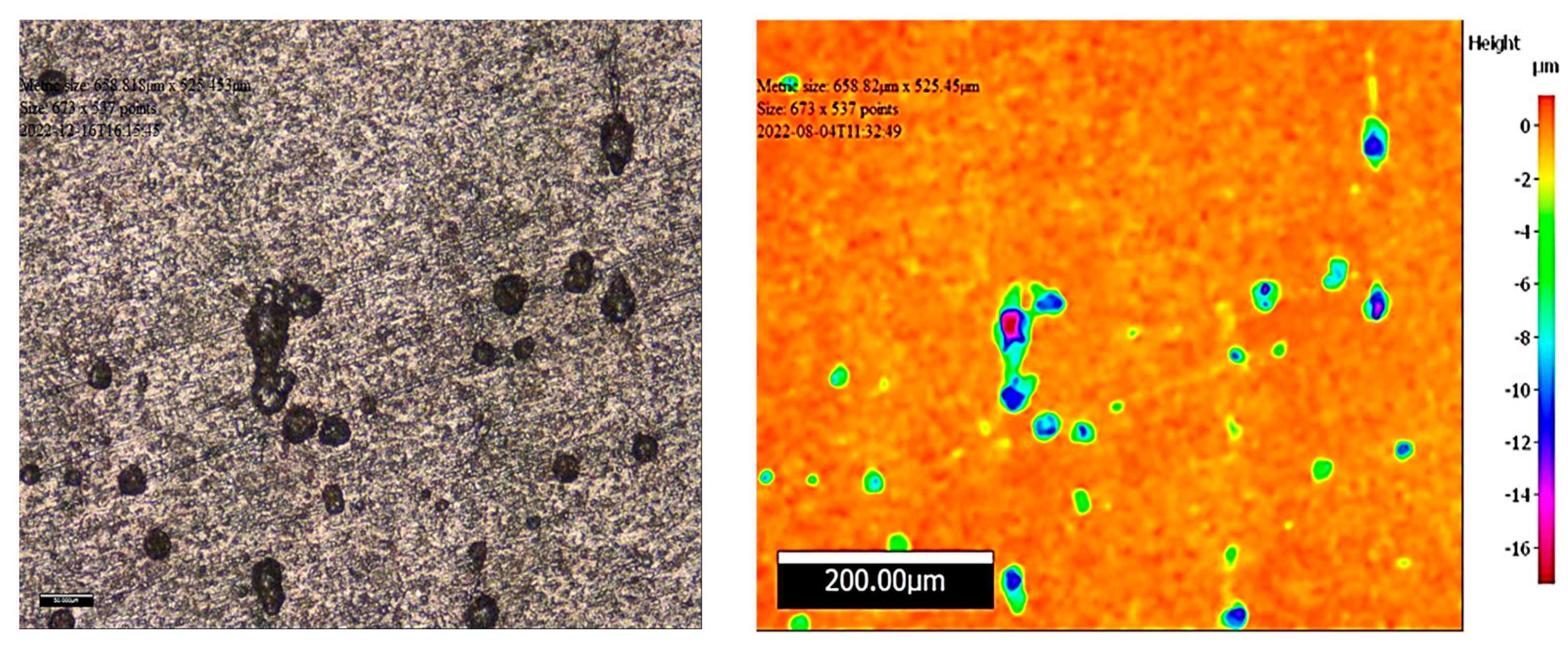
2.4. Post-Test Surface Analysis

Clarke’s solution, developed per ASTM standard G1, was used to strip the samples of any remaining adhering products on the steel surfaces; also, ultrapure water (resistivity of 18.2 MΩ.cm) was used to clean the samples after testing to remove any stray corrosion products as shown in Figure 2. After nitrogen drying, the samples were placed in a vacuum desiccator until further analyses were performed. Finally, a 3D profile of the corroded samples and the necessary morphological characteristics were acquired using surface profilometry (Infinite Focus, Alicona Instruments, Graz, Austria).

2.5. Data Analysis Procedures

• The raw EN data (obtained from carbon steel samples from the 172,800 dataset) were broken down into 2048-point segments.
• In total, there were approximately 84 individual parts. In addition, linear regression was used to remove trends from the EN sections.
• Post-analysis was performed for the three sets of experimental ENC data using the discrete wavelet transform (R1: passivation, R2: uniform, and R3: pitting).
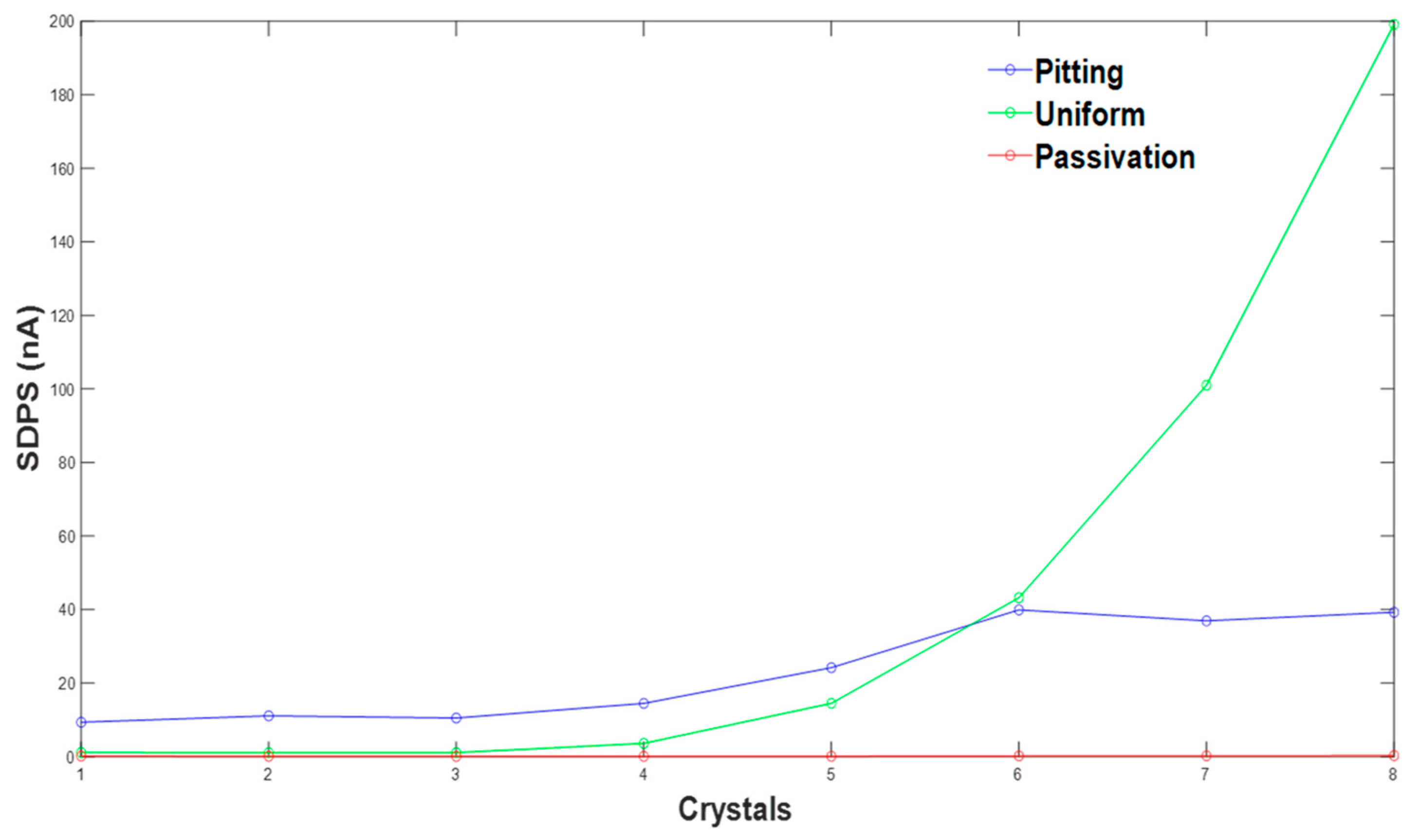
• Wavelet transform analysis was used to set coefficients, which were used to construct EDPs and SDPS (standard deviation of partial signals).
• Image encoding of the segments by means of wavelet scalograms, as discussed in the next two sections.

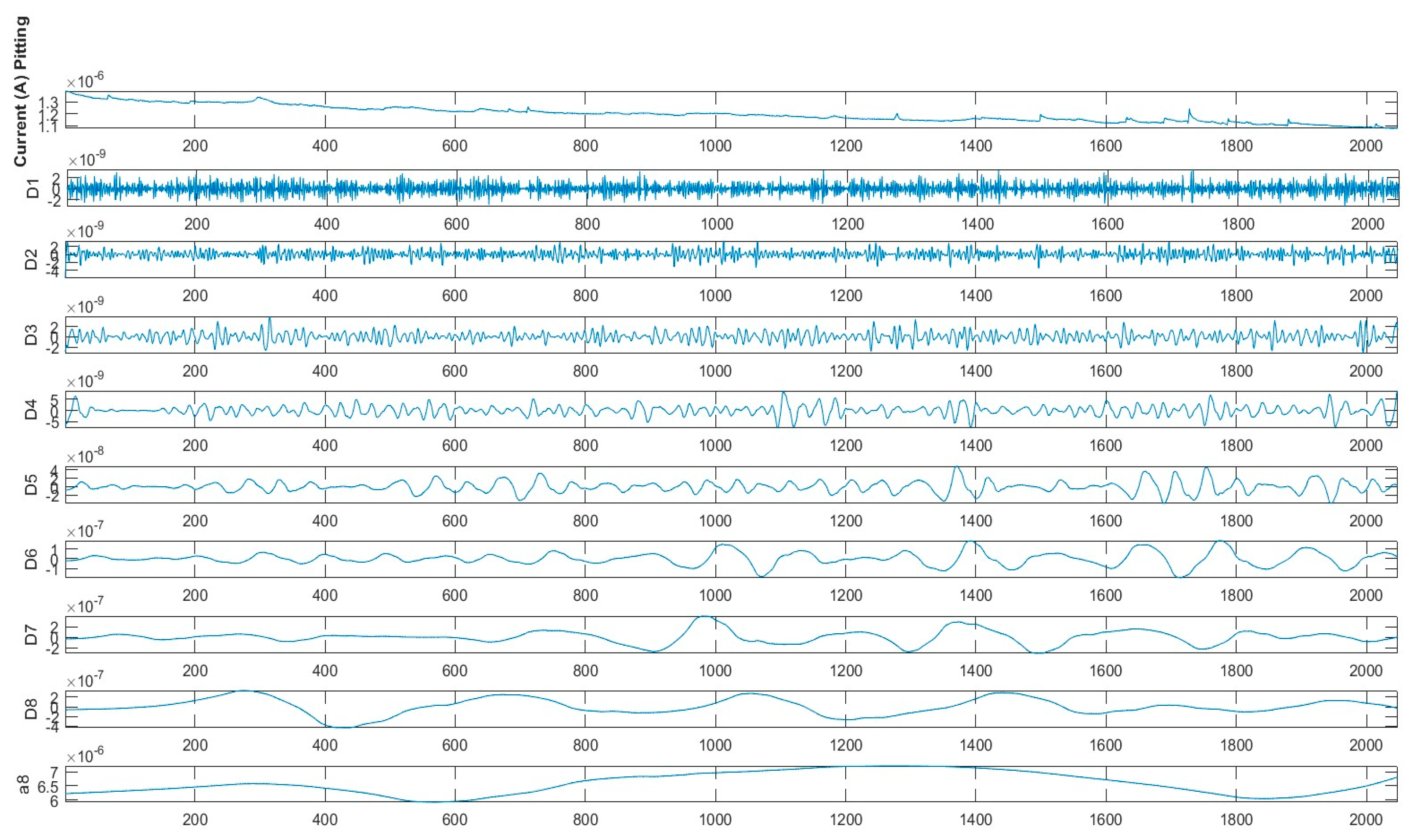
2.5.1. Discrete Wavelet Analysis

When analyzing discrete signals, discrete wavelet transform (DWT) is often employed because of its efficiency in calculating the coefficient values of various frequency bands for each time window. This information is produced by combining the sampled signal with functions that are extended and shifted copies of a wavelet function (or mother wavelet). The raw data can be represented as a weighted sum of wavelet functions (d_j,n(t) and d_j,n(t)) with detail (d_j,n) and smooth (s_j,n) coefficients, respectively. Although the coefficients obtained by DWT can be difficult to interpret for ECN signals, they imply a correlation between the wavelet function and relevant signal segment [19,21]. The concept of coefficient energy distribution can be used to make sense of wavelet transform findings for analyzing electrochemical noise. In this scenario, the energy contribution of each decomposition level is determined with respect to the overall energy of the signal (which may be determined using the equations presented in [21,22]) as follows [23]:

$$E={{\displaystyle \sum }}_{n=1}^N{x}_n^2, n = 1, 2, \dots \mathit{N}$$

(1)

$$E_j^d=1/E{{\displaystyle \sum }}_{n=1}^{N/2j}{d}_{j,n}^2, j = 1, 2, \dots \mathit{J}$$

(2)

$$E_j^S=1/E{{\displaystyle \sum }}_{n=1}^{N/2j}{S}_{j,n}^2, n = 1, 2, \dots \mathit{N}$$

(3)

2.5.2. Wavelet Scalogram and Machine Learning Approach

• Signal preprocessing: Preprocessing and segmentation of the noise signal was performed with a moving window defined by window length (b) and step size (s). In this investigation, the step size was set as equal to the window size (s = b), which yielded a series of non-overlapping or contiguous time series segments.
• Image encoding of the segments by means of wavelet scalograms: Encoding time series signals into images using wavelet scalograms is a technique that transforms time-domain data into a visual representation suitable for analysis by machine learning algorithms or human observers [24]. A relatively novel approach that has emerged to take advantage of the availability of pretrained deep learning neural networks, such as convolutional neural networks (CNNs), is to convert signals to images that can be directly presented to these networks for classification [9,24]. This is accomplished by splitting the signal into contiguous segments that can be imaged individually.
• As a first step, the time series signal is decomposed into different frequency components, revealing both low- and high-frequency variations present in the data. The wavelet transforms result in a set of coefficients, which are used to construct a scalogram, essentially a two-dimensional representation, where one axis represents time (or position in the signal) and the other axis represents the scale (or frequency). The amplitude of wavelet coefficients at each time and scale position is typically represented using colors. Brighter colors, such as yellow or white, are used to depict higher amplitudes, while darker colors represent lower amplitudes. Each point in this image corresponds to a specific time and frequency information from the original time series signal.
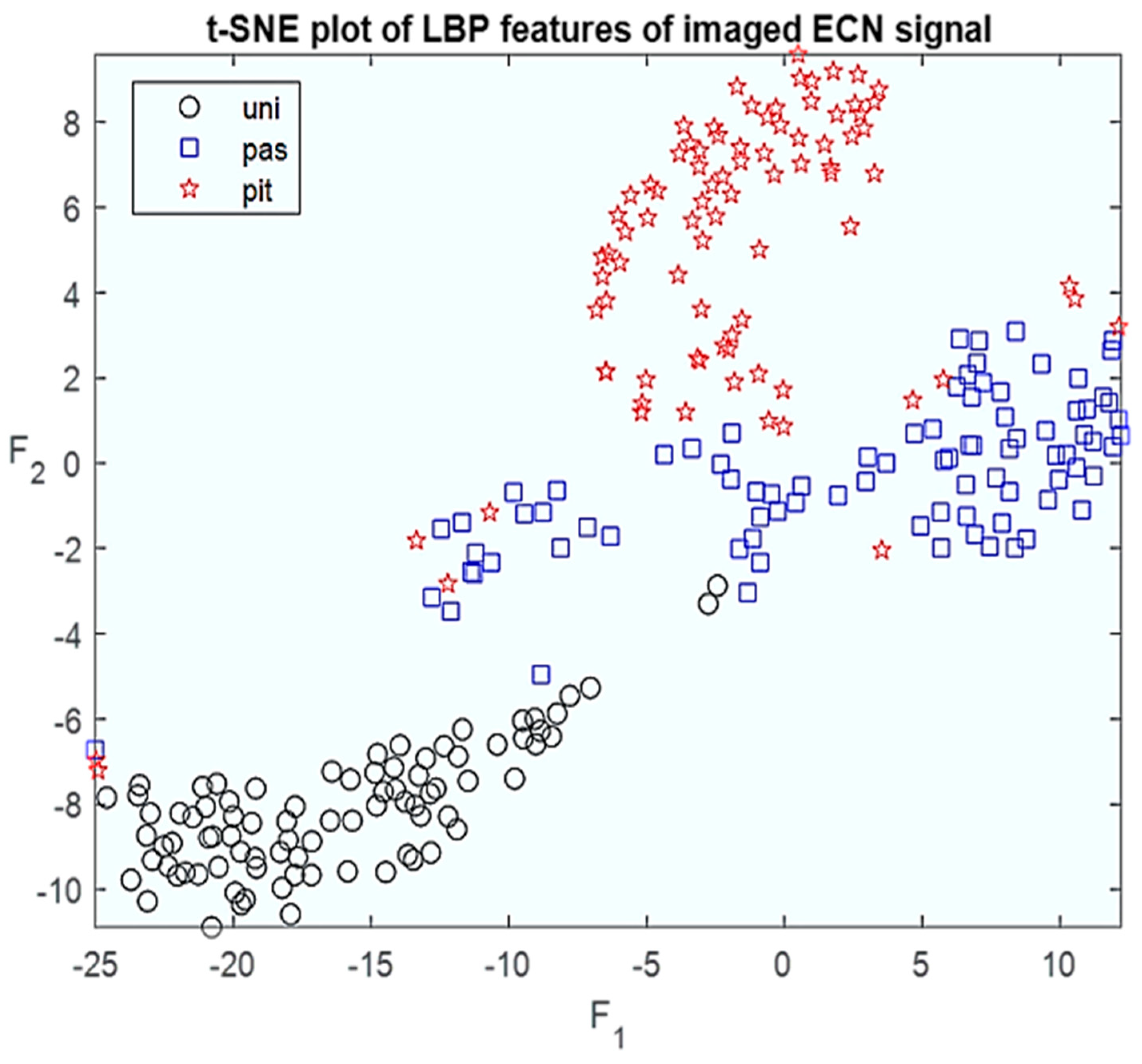
• Feature extraction with local binary patterns (LBPs): An LBP is a texture descriptor that operates on individual pixels or small neighborhoods within an image. It does so by comparing the intensity of a central pixel to its neighboring pixels. More specifically, for each pixel in the image, a local neighborhood is defined. This neighborhood typically consists of a circular or square region of pixels around the central pixel.
• Within the local neighborhood, the LBP compares the intensity value of the central pixel to the intensity values of its neighboring pixels. This comparison is binary, meaning that each neighbor is assigned a binary value (0 or 1) based on whether its intensity is greater or less than that of the central pixel. The binary values obtained from the comparisons are concatenated to form a binary pattern. For example, if you have an 8-pixel neighborhood, you will obtain an 8-bit binary pattern. The LBP is applied to each pixel in the image, resulting in a corresponding binary pattern for each pixel. These binary patterns are then used to create a histogram of patterns for the entire image. The LBP histogram is a representation of the distribution of texture patterns within the image and serves as a feature vector that characterizes the texture properties of the image.
• Corrosion control chart: Finally, these features can be projected into a corrosion monitoring and control chart after reducing the dimension of the local binary pattern vectors. The analytical methodology for corrosion control is summarized in Figure 3.

3. Results and Discussion

3.1. Surface Morphology Analysis

After conducting EN tests, the electrode surfaces were examined using a 3D optical microscope to determine their morphology. Th corresponding behavior was observed on the electrode surfaces in the solutions selected to generate uniform and passive tests. However, the surface conditions differed between the electrodes in the pitting test. As shown in Figure 4 and Figure 5, there were noticeably fewer pits on specimen (S1) following immersion. Measurements taken again on the other specimen (S2) revealed large pit areas, as illustrated in Figure 6. The S2 working electrode, in contrast to S1, included numerous deep defects. As shown also in Figure 6, after 24 h of immersion for the pitting test run, the maximum pit depth with working electrode S2 was approximately 55 µm. As a group, all pits followed the same general pattern in terms of their shape and size. (More details for SEM analysis and an extra description for figures are provided as supplementary data.)

3.2. Post-Data Processing and Analysis

Figure 7 displays the linear regression-detrended electrochemical noise (EN) data for the three tests of corrosion listed in Table 2. The electrochemical current and potential signals exhibited varying behaviors for various corrosion systems, as shown in Figure 7. During the uniform corrosion test period, high-frequency variations were detected in both potential and current noise levels. The maximum potential amplitude was −685 mV vs. Ag/AgCl; the maximum current amplitude was about −16 × ${10}^{-3}$ mA. In most cases, as depicted in Figure 7, it is impossible to display any noticeable transitory peaks. For the first three hours of monitoring, current noise in the case of pitting corrosion had high peaks and amplitude (about −2.4 × ${10}^{-3}$ mA). After that, as seen in Figure 7, the current signal peaked in a manner that is characteristic of metastable pitting, with a sharp increase followed by a sharp decrease. For example, it has been observed that the frequencies of noise signals associated with uniform corrosion processes are higher than those associated with localized corrosion [20]. In comparison, the EN signals generated by the passivation test exhibited much lower variability, with maximum amplitudes of −20 × ${10}^{-3}$ mA and −70 mV.

In general, uniform corrosion, which affects the entire metal surface, proceeds faster than localized corrosion. In other words, the charge transfer process, which is a transient phase, is primarily responsible for determining the uniform corrosion process. This implies that high-frequency signals predominate in the EN spectrum. Therefore, the EN has a large amount of energy in the form of high-frequency signals. However, the EN spectrum reveals that pitting corrosion has a lower fluctuation frequency than uniform corrosion. Consequently, the EN spectrum during localized corrosion is mainly composed of low-frequency signals. Thus, the energy distribution plots (EDP) were used as “fingerprints” of the corrosion behavior carried by the EN signals.

To analyze the 172,800 datasets, first the DWT was used individually for each system to break them down after segmentation, as shown as an example in Figure 8. The energy distribution (ED) plots and standard deviations of the partial signal (SDPS) for runs R1 through R3 were then obtained and are displayed in Figure 9 and Figure 10.

The wavelet transform involves first segmenting the signal and then applying the transform to each sub-segment. To achieve this, we considered a window in which a wavelet with a certain time width was contained [22]. Therefore, wavelet coefficients were used to quantify the degree to which different parts of the signal were similar to one another. We needed a Wavelet Analyzer Toolbox to extract EDPs from the EN data. A prior discrete wavelet transform (DWT) was implemented with an eight-level decomposition with a Daubechies 4 wavelet, as shown in Figure 8, for the passivation of current signals.

Figure 8. An example of DWT implying to the current raw data for EN, e.g., pitting.

Figure 8. An example of DWT implying to the current raw data for EN, e.g., pitting.

3.2.1. EDP

In this study, eight details and one approximation were used to analyze the number of crystals [21], which refers to specific patterns or structures that emerge in the wavelet coefficients or scalogram of a signal. Crystals indicate regions in the time–frequency plane where the wavelet coefficients exhibit distinct patterns or high energy concentrations. These patterns can help identify important features, such as sharp transitions or oscillatory behavior within the signal.

Figure 9a shows an EDP plot derived from the EN data, where the current noise signal represents three different corrosion tests. With 2048 data points, overall, Figure 9 reveals that most of the carbon steel wavelets’ energy was concentrated at a high frequency. The greatest “Pitting” signal is in the coarser crystal d8. In contrast, high values at a large scale may be associated with transients [25], as in “Uniform” current signals; practically, the energy is accumulated in the smooth coefficients d7-d8 with the highest energy value in d8. However, the high-energy value at d6 is clearly displayed in “Pitting” current signals via the EDP of partial signals (PSs) as shown in Figure 9b, which is a process that occurs on a medium time scale. This may suggest that a “Uniform” current signal is dominated by a process with a time constant longer than that underlying a “Pitting” signal [20]. In the final case, the “Passivation” current signal, the energy is primarily stored in the coarse crystal d8 in the event of a signal with slow fluctuation.

In the time series of recording, it has been pointed out that rapid fluctuations are linked to high values in finer crystals (smaller time scale), whereas transients are linked to high values on larger scales [20]. In general, it is suggested that when energy is collected on the initial crystals (d1–d3), it is due to a metastable pitting process; when primary energy is present on the crystals from d4 to d6, it is due to localized corrosion (pitting); and if energy is present in the coarse crystals d7 and d8, it is due to a diffusion, generalized, or controlled process, as shown in Figure 11 [25].

The results may demonstrate that there is energy buildup in crystals d7 and d8, crystal S8 is connected to DC, and approximation-based crystals cannot exhibit DC energy. When the d8 crystal has the maximum energy accumulation, which is due to the formation of a passive film, according to Shahidi et al. [19], the higher energies in crystals d4, d5, and d6 are correlated with a re-passivation process. Finally, utilizing the EDP from the EPN signal in which the potential noise signal corresponds to three corrosion systems reveals that there is an increase in energy proportional to the scale, which becomes more substantial beginning with the d6 crystal [19].

Figure 9. (a) The energy distribution plot (EDP) for each corrosion test in DWT (supervised monitoring), e.g., segment one based on coefficients of details; (b) the energy distribution plot (EDP) for each corrosion test in DWT, e.g., segment one based reconstructed partial signals.

Figure 9. (a) The energy distribution plot (EDP) for each corrosion test in DWT (supervised monitoring), e.g., segment one based on coefficients of details; (b) the energy distribution plot (EDP) for each corrosion test in DWT, e.g., segment one based reconstructed partial signals.

Figure 10. The standard deviation of partial signals (SDPS) for each corrosion test, e.g., segment one.

Figure 10. The standard deviation of partial signals (SDPS) for each corrosion test, e.g., segment one.

Figure 11. Schematic representation of the information that may be obtained from an EDP [4,26]. Reprinted with permission from Ref. [26]. 2012, Homborg, A.M., et al.

Figure 11. Schematic representation of the information that may be obtained from an EDP [4,26]. Reprinted with permission from Ref. [26]. 2012, Homborg, A.M., et al.

3.2.2. Standard Deviation of Partial Signals (SDPS)

Collectively, the wavelet coefficients allow for the reconstruction of the original signal. One smooth signal, S_J(t), and j detail signals, D_j, were produced using the inverse DWT (t). A “partial signal” (PS) is any one of these j + 1 signals ([19,27]). In this context, a frequency-specific PS is a signal that faithfully reproduces the amplitude and phase shifts of the original signal [14]. Fluctuations in the intensity of PS around its mean, as measured by its SDPS, may be indicative of the degree of electrochemical activity on the electrode surface at a given frequency. Figure 10 shows a plot of SDPS versus the names of the crystals to which they correspond for the three corrosion tests. This indicates that the SDPS plot, but not the ED plot [22], can classify multiple signals according to their intensity and the number of spikes they represent.

When comparing the ED and SDPS plots as wavelet features for the EN data, both plots can identify distinct frequencies within a single signal based on their relative intensities [19]. Therefore, the dominant frequency of a single signal can be identified using either the ED or SDPS plot. Hence, the ED plot, when used in combination with the SDPS plot, may provide insight into the electrochemical behavior of a corroding system in ways that the latter alone cannot. Because of this agreement in peak location between the ED and SDPS plots, it is reasonable to employ the latter in analyzing EN measurement records. However, it appeared that the SDPS plot was more adaptable than the ED plot for corrosion monitoring. Corrosion severity can be quantified using the SDPS plot, which is an attractive feature [19]. A quantitative analysis of these results can be used to develop automatic monitoring systems for corrosion control, as discussed in the next section.

3.3. Feature Extraction for the Monitoring of Corrosion

Several methods can be used to extract features from time series data, such as electrochemical noise signals associated with pitting, passivation, and uniform corrosion, as conducted earlier in some studies. As discussed in the Methods section, in this study, the electrochemical corrosion signals shown in Figure 12 were segmented, setting b = s = 2048. This resulted in 84 segments representing each type of corrosion. These signals were subsequently converted into wavelet scalograms, examples of which can be seen in Figure 13.

Figure 13 shows the wavelet spectrograms of these segments, each of which contains 40 samples of electrochemical noise signals for uniform corrosion, passivation, and pitting corrosion. For illustrative purposes, a well-established approach to extracting features from images, based on the concept of local binary patterns, was used to extract features from these wavelet images. The results for the images based on a sample length of 500 are shown in Figure 14. Each marker in the figure represents an image or, equivalently, a time series segment. Markers of different colors were used to visualize the features in a t-stochastic neighbor embedding (t-SNE) score plot [28]. t-SNE is a dimensionality reduction technique commonly used for visualizing high-dimensional data in lower-dimensional spaces. It preserves the pairwise similarities between data points as best as possible by modelling them as probabilities in both the high- and low-dimensional spaces. This method is particularly effective for revealing clusters and patterns in data, making it a popular choice for visualizing complex datasets and understanding the inherent structures within them. As can be seen from the scatterplot of the t-SNE features (F₁ and F₂) in in Figure 14, different corrosion systems can be separated with a degree of accuracy exceeding 90%.

Such a plot can be used directly for online monitoring of the type of corrosion that occurs. In this case, it would first require the construction of a suitable model to map the LBP features of the images to their corresponding t-SNE features. In the second step, samples collected in batches of 40 would be converted into wavelet spectra and new LBP features extracted from these new images. Finally, these LBP features could then be mapped to the t-SNE chart shown in Figure 14. Depending on the location of the mapped data, it would then be possible to infer the type of corrosion that is taking place.

Figure 14. Visualization of LBP features of the wavelet images of the time series segments (length = 500 samples).

Figure 14. Visualization of LBP features of the wavelet images of the time series segments (length = 500 samples).

4. Conclusions

The present work addresses electrochemical noise analysis as a valuable technique for online corrosion monitoring in an aqueous environment to improve subsequent data analysis using machine learning models, and this study introduces online monitoring of the type of corrosion taking place:

• A tool was designed to aid EN analysis by automatically prioritizing statistically optimal ECN by combining wavelet spectra and LBP features.
• Micro-surface analysis and electrochemical noise signals were used to determine the different forms of corrosion and their characteristics on metal surfaces.
• Resistance to electrochemical noise and features extracted from discrete wavelet transform such as ED and SDPS were found to be quantifying some types of corrosion, in experimental and analytical results, and using wavelet transform features can be a step further for comparisons with a developed model of the wavelet scalogram images.
• The findings of this study emphasize the necessity of employing a wavelet transform based on a wavelet scalogram for analyzing electrochemical noise, and that combining deep learning approaches is valuable for online monitoring.
• This study provides a possible way to develop this tool of monitoring to enhance outcomes using just one type of signal, reducing the equipment required to gather data in various scopes of work, such as unsupervised monitoring.

References

1. McLaughlin, K. Corrosion monitoring. Anti -Corrosion Methods Mater 2000, 47, 26–29. [Google Scholar] [CrossRef]
2. Roberge, P.R. Maintenance, Management, and Inspection Strategies. In Corrosion Inspection and Monitoring; Wiley: Hoboken, NJ, USA, 2007; pp. 79–187. [Google Scholar] [CrossRef]
3. Roberge, P.R. Corrosion Detectability. In Corrosion Inspection and Monitoring; Wiley: Hoboken, NJ, USA, 2007; pp. 27–78. [Google Scholar] [CrossRef]
4. Obot, I.B.; Onyeachu, I.B.; Zeino, A.; Umoren, S.A. Electrochemical noise (EN) technique: Review of recent practical applications to corrosion electrochemistry research. J. Adhes. Sci. Technol. 2019, 33, 1453–1496. [Google Scholar] [CrossRef]
5. Papavinasam, S. Electrochemical polarization techniques for corrosion monitoring. In Techniques for Corrosion Monitoring, 2nd ed.; Yang, L., Ed.; Woodhead Publishing: Cambridge, UK, 2021; pp. 49–85. [Google Scholar] [CrossRef]
6. Martinelli-Orlando, F.; Angst, U. Monitoring corrosion rates with ER-probes—A critical assessment based on experiments and numerical modelling experiments and numerical modelling. Corros. Eng. Sci. Technol. 2022, 57, 254–268. [Google Scholar] [CrossRef]
7. Hou, Y.C.; Aldrich Lepkova, K.; Kinsella, B. Detection of under deposit corrosion in a CO2 environment by using electrochemical noise and recurrence quantification analysis. Electrochim. Acta 2018, 274, 160–169. [Google Scholar] [CrossRef]
8. Eden, D. Electrochemical Noise—The First Two Octaves. In Proceedings of the CORROSION 98, San Diego, CA, USA, 22–27 March 1998. paper 386. [Google Scholar]
9. Hou, Y.; Aldrich, C.; Lepkova, K.; Machuca, L.L.; Kinsella, B. Analysis of electrochemical noise data by use of recurrence quantification analysis and machine learning methods. Electrochim. Acta 2017, 256, 337–347. [Google Scholar] [CrossRef]
10. Hou, Y.; Pojtanabuntoeng, T.; Iannuzzi, M. Use of electrochemical current noise method 413 to monitor carbon steel corrosion under mineral wool insulation. NPJ Mater. Degrad. 2020, 4, 39. [Google Scholar] [CrossRef]
11. Corrosion of Weldments. Microstructures, Basic Understanding of Weld Corrosion. In Corrosion of Weldments; ASM International: Almere, The Netherlands, 2021; pp. 1–12. [Google Scholar] [CrossRef]
12. Liao, X.; Qiang, B.; Wu, J.; Yao, C.; Wei, X.; Li, Y. An improved life prediction model of 418 corrosion fatigue for T-welded joint. Int. J. Fatigue 2021, 152, 106438. [Google Scholar] [CrossRef]
13. Xia, D.-H.; Song, S.Y.; Behnamian, Y.; Hu, W.; Cheng, Y.; Luo, F.J.-L.; Huet, F. Review—Electrochemical Noise Applied in Corrosion Science: Theoretical and Mathematical Models towards Quantitative Analysis. J. Electrochem. Soc. 2020, 167, 081507. [Google Scholar] [CrossRef]
14. Legat, A.; Dolecek, V. Corrosion Monitoring System Based on Measurement and Analysis of Electrochemical Noise. Corrosion 1995, 51, 295–300. [Google Scholar] [CrossRef]
15. Comas, C.; Huet, F.; Ngo, K.; Idrissi, H.; Normand, B. Corrosion propagation monitoring using electrochemical noise measurements on carbon steel in hydrogenocarbonated solution containing chloride ions. Corros. Sci. 2021, 193, 109885. [Google Scholar] [CrossRef]
16. Al-Mazeedi, H.A.; Cottis, R.A. Parameter Maps for the Assessment of Corrosion Type 427 from Electrochemical Noise Data. In Proceedings of the Corrosion Conference, NACE International, New Orleans, LA, USA, 28 March 2004; paper 4460. pp. 1–10. [Google Scholar]
17. Xia, D.; Song, S.; Wang, J.; Shi, J.; Bi, H.; Gao, Z. Electrochemistry Communications Determination of corrosion types from electrochemical noise by phase space reconstruction theory. Electrochem. Commun. 2012, 15, 88–92. [Google Scholar] [CrossRef]
18. Xia, D.; Song, S.; Behnamian, Y.; Xia, D.; Song, S.; Behnamian, Y. Detection of corrosion degradation using electrochemical noise (EN): Review of signal processing methods for identifying corrosion forms. Corros. Eng. Sci. Technol. 2016, 51, 2782. [Google Scholar] [CrossRef]
19. Shahidi, M.; Hosseini, S.M.A.; Jafari, A.H. Comparison between ED and SDPS plots as the results of wavelet transform for analysing electrochemical noise data. Electrochim. Acta 2011, 56, 9986–9997. [Google Scholar] [CrossRef]
20. Aballe, A.; Bethencourt, M.; Botana, F.J.; Marcos, M. Using wavelets transform in the analysis of electrochemical noise data. Electrochim. Acta 1999, 44, 4805–4816. [Google Scholar] [CrossRef]
21. Aballe, A.; Bethencourt, M.; Botana, F.J.; Marcos, M.; Sa, J.M. Use of wavelets to study electrochemical noise transients. Electrochim. Acta 2001, 46, 2353–2361. [Google Scholar] [CrossRef]
22. Mallat, S. A wavelet tour of signal processing. In The Sparse Way, 3rd ed.; Academic Press: Burlington, MA, USA; Elsevier: Burlington, MA, USA, 2009. [Google Scholar]
23. Marques, L.; Romulo, A.; Cotta, A.; Marques Côco, P.K.F.; Samatelo, J.L.A.; Salles, E.O.T. Identification of Corrosive Substances and Types of Corrosion Through 449 Electrochemical Noise Using Signal Processing and Machine Learning. J. Control Autom. Electr. Syst. 2019, 30, 16–26. [Google Scholar] [CrossRef]
24. Aldrich, C. Process fault diagnosis for continuous dynamic systems over multivariate 465 time series. In Time Series Analysis; Ngan, C.-K., Ed.; IntechOpen: London, UK, 2019; ISBN 978-953-51-7827-9. [Google Scholar]
25. Jáquez-Muñoz, J.M.; Gaona-Tiburcio, C.; Cabral-Miramontes, J.; Nieves-Mendoza, D.; Maldonado-Bandala, E.; Olguín-Coca, J.; López-Léon, J.L.D.; De Los Rios, J.P.F.; Almeraya Calderón, F. Electrochemical noise analysis of the corrosion of titanium alloys in NaCl and H2SO4 solutions. Metals 2021, 11, 105. [Google Scholar] [CrossRef]
26. Homborg, A.M.; Tinga, T.; Zhang, X.; Van Westing, E.P.M.; Oonincx, P.J.; De Wit, J.H.W.; Mol, J.M.C. Time-frequency methods for trend removal in electrochemical noise data. Electrochim. Acta 2012, 70, 199–209. [Google Scholar] [CrossRef]
27. Shahidi, M.; Jafari, A.H.; Hosseini, S.M.A. Comparison of symmetrical and asymmetrical cells by statistical and wavelet analysis of electrochemical noise data. Corrosion 2012, 68, 1003–1014. [Google Scholar] [CrossRef] [PubMed]
28. Van der Maaten, L.; Hinton, G. Visualizing Data using t-SNE. J. Mach. Learn. Res. 2008, 9, 2579–2605. [Google Scholar] [CrossRef]
Figure 1. Diagrammatic configuration for the electrochemical noise measurements.
Metals 14 00066 g001
Figure 2. The two working electrodes after cleaning.
Metals 14 00066 g002
Figure 3. Analysis of electrochemical noise signals by means of wavelet scalogram.
Metals 14 00066 g003
Figure 4. Two-dimensional morphologies of specimen 1 (S1) after immersion for uniform condition.
Metals 14 00066 g004
Figure 5. Another area of (S1) morphologies after immersion for uniform condition.
Metals 14 00066 g005
Figure 6. Specimen 2 (S2) after immersion for pitting condition showing deep pits.
Metals 14 00066 g006
Figure 7. The original raw EN data signals for the three tests of corrosion: passivation, pitting, and uniform.
Metals 14 00066 g007
Figure 12. Electrochemical noise signals associated with unform corrosion (top), pitting corrosion (middle), and passivation (bottom) after being segmented.
Metals 14 00066 g012
Figure 13. Wavelet scalogram images of ECN time series segments showing the magnitudes of the wavelet coefficients as a function of time and scale.
Metals 14 00066 g013