Electrical Equivalent Circuit Model Prediction of High-Entropy Alloy Behavior in Aggressive Media

Abstract

Due to the optimistic outcomes of the research on high-entropy alloys, new designs of these alloys are being encouraged. We studied the high-entropy CoCrFeMoNi alloy and the CoCrFeMoNi alloy doped with Zr. In order to choose the best electrical equivalent circuit for the prediction of the behavior of these high-entropy alloys at various potentials in artificial seawater, electrochemical impedance spectroscopy (EIS) measurements were conducted on samples with and without Zr-doped CoCrFeMoNi. At various potential levels, the impedance spectra were measured between −1.0 and +0.8 V vs. SCE. The study consists of a preliminary section with microstructure by metallography, open-circuit potential, and linear polarization curves by direct-current tests followed by visual analysis of the impedance spectra, and, finally, the selection of an equivalent electrical circuit model to fit the experimental data. By leveraging the advantages of EIS analysis, the information is essential for materials development, corrosion-mitigation strategies, and the successful implementation of these alloys in practical applications. It is important to note that selecting an equivalent circuit is often an iterative and subjective process, as it involves a balance between model complexity and the ability to accurately represent the system’s behavior.

1. Introduction

Electrochemical impedance spectroscopy (EIS) is a technique used to analyze the electrical properties of electrochemical systems. It provides valuable information about the interfacial processes occurring at the electrode–electrolyte interface [1]. In EIS, a small sinusoidal perturbation signal is applied to the electrochemical system over a range of frequencies and the response of the system is then measured, typically in terms of impedance, which is the ratio of the applied voltage to the resulting current. The impedance measured in EIS consists of two components: real (resistance) and imaginary (reactance) parts. The real part represents the system’s resistance to the flow of charge, while the imaginary part reflects the system’s capacitive or inductive behavior.

By varying the frequency of the applied signal, EIS generates an impedance spectrum that provides insights into various electrochemical processes. This includes information about charge transfer reactions, adsorption/desorption processes, diffusion of species, and other phenomena occurring at the electrode–electrolyte interface. EIS is widely used in various fields, including biomaterials [2,3,4], fuel cells [5,6,7], the chemical industry [8,9,10,11], etc., to characterize and understand the behavior of electrochemical systems. The obtained impedance data can be further analyzed and modeled to extract valuable parameters and gain insights into the underlying electrochemical processes. The use of advanced impedance measurement setups and dedicated software has accelerated experiments in the field of EIS. As a result, data acquisition is no longer the time-consuming aspect of the process; rather, the analysis of experimental data has become the primary bottleneck. Therefore, impedance modeling plays a crucial role in the EIS method [12,13,14,15].

The kinetic approach to EIS modeling, which is well-established and documented in various textbooks [16,17], is commonly used. This approach involves linearizing nonlinear equations of electrochemical kinetics by utilizing small perturbation signals. The linearized equations are then subjected to Laplace transformation, along with differential equations and partial derivatives equations derived from adsorption and mass transport processes, respectively [18].

The analysis of corrosion behavior of a new high-entropy alloy with electrochemical impedance spectroscopy (EIS) offers several advantages:

Non-destructive characterization: EIS is a non-destructive approach, allowing for the analysis of corrosion behavior without causing harm to or changing the material being investigated. When examining innovative or expensive high-entropy alloys, this is especially helpful because it allows for many measurements to be taken on the same sample, producing useful information while preserving the material for additional study or applications.

Comprehensive electrochemical information: In-depth electrochemical knowledge on the corrosion behavior of high-entropy alloys is provided by EIS. It provides information about a number of electrochemical processes that take place at the alloy’s surface, including mass transport, double-layer capacitance, and adsorption/desorption phenomena. This enables a thorough comprehension of the mechanisms causing corrosion and the variables affecting an alloy’s corrosion resistance.

Quantitative assessment of corrosion resistance: The quantitative evaluation of corrosion resistance characteristics is possible with EIS. Important corrosion parameters, such as polarization resistance, corrosion rate, capacitance, and impedance components, can be retrieved by fitting the experimental impedance data to the relevant equivalent circuit models. These variables offer measurable indicators of the alloy’s resistance to corrosion, facilitating performance assessment and material comparison.

Sensitivity to localized corrosion: For high-entropy alloys, localized corrosion processes, such as pitting or crevice corrosion, are of significant importance and EIS can shed light on these phenomena. EIS can identify and describe localized corrosion processes by examining the impedance spectrum and keeping track of changes in the low-frequency range, which helps determine the alloy’s susceptibility to these types of corrosion.

Evaluation of protective coatings or treatments: EIS is frequently used to assess the efficacy of surface treatments or protective coatings on high-entropy metals. It is feasible to evaluate the barrier qualities, adherence, and long-term performance of the protective layers by contrasting the impedance responses of coated and untreated samples. This knowledge is essential for boosting high-entropy alloy durability and corrosion protection strategies for practical applications.

Fast and efficient data acquisition: EIS experiments can be performed relatively quickly, allowing for efficient data acquisition. With modern high-performance impedance-measurement setups and dedicated software, a significant number of experiments can be conducted within a few laboratory days. This rapid data acquisition facilitates the screening and comparison of different high-entropy alloys or the evaluation of corrosion behavior under various conditions.

Taking into account all these, the purpose of our study is to select the proper electrical equivalent circuit for the prediction of the behavior of two high-entropy alloys at different potentials in artificial seawater. The study consists of three sections: (1) a preliminary section with microstructure by metallography, open-circuit potential, and linear polarization curves by direct current tests; (2) visual analysis of the impedance spectra; and (3) selection of an equivalent electrical circuit model to fit the experimental data. By leveraging the advantages of EIS analysis, the information is essential for materials development, corrosion-mitigation strategies and the successful implementation of these alloys in practical applications.

2. Materials and Methods

2.1. Samples Preparation

The CoCrFeMoNi alloy (Sample 1) and the Zr-doped CoCrFeMoNi alloy (Sample 2) were investigated in this study. The samples were produced by the ERAMET Laboratory at the Politehnica University of Bucharest using a vacuum arc remelting (VAR) system, model MRF ABJ 900. The laboratory carefully considered potential losses due to vaporization and the expected incorporation of chemical elements during the melting process to design the metallic charge.

To ensure high purity, raw materials with a minimum purity of 99.7% for Co, Cr, Fe, Mo, Ni, and Zr were utilized. To achieve uniformity, the resulting alloys underwent eight cycles of flipping and remelting in the VAR equipment, with four repetitions for each part.

The elemental composition of both Sample 1 and Sample 2 was determined through energy-dispersive X-ray analysis (EDS). This analysis was conducted using a Fei XL30 ESEM scanning electron microscope (MTM, Leuven, Belgium) equipped with an EDAX Sapphire detector (EDAX Inc, Pleasanton, CA, USA), allowing for accurate characterization of the alloy’s elemental information, presented in

Table 1. The results in wt% of EDS analysis of the alloy Sample 1 and Sample 2.

wt%	Sample 1	Sample 2
Co	19.81	19.53
Cr	19.98	19.02
Fe	18.04	17.84
Mo	25.18	26.36
Ni	16.99	17.12
Zr	-	0.13

. The steps of the sample´s preparation are presented in Figure 1 and explained in our work where also the mechanical properties and corrosion behavior of the samples at corrosion potential were previously studied [19].

2.2. Electrochemical Measurements

Three electrodes were used in a typical electrochemical cell setup for all the tests that were performed. A working electrode, a reference electrode, and a counter electrode are included in this arrangement. The working electrode (Samples 1 and 2) is constructed of the alloy under investigation and is where the electrochemical reaction of interest takes place. It provides a platform for studying the behavior of the material. The reference electrode serves as a reference point for potential measurements and maintains a stable potential. In this study, a saturated calomel electrode (SCE) was employed as the reference electrode due to its well-known potential (+0.242 V). The counter electrode is an inert electrode that completes the electrical circuit and facilitates the balanced flow of electrons. Platinum, an inert material that does not participate in the electrochemical reaction, was chosen as the counter electrode in this case. The working electrode and the counter electrode conduct current via the electrolyte solution, which, in this case, is a 3.5% NaCl solution replicating a marine environment, throughout the electrochemical reaction. To ascertain the system’s electrochemical properties, the potential difference between the working electrode and the reference electrode is measured. The reference electrode ensures correct potential measurements, while the three-electrode arrangement ensures exact evaluations of the electrochemical behavior. By utilizing this configuration and employing the appropriate electrolyte solution, the study aimed to investigate and characterize the electrochemical response and corrosion behavior of the alloy samples in a simulated seawater environment. The tests were conducted using a Biologic SP-150 potentiostat, manufactured in Seyssinet-Pariset, France. To control the experimental conditions and establish the necessary process parameters, the EC-Lab^® v-9.55 program (BioLogic Science Instruments SAS, Seyssinet-Pariset, France) was employed. This software provided the required functionalities for executing the corrosion techniques and ensuring accurate measurements and data acquisition during the tests.

2.3. Preliminary Tests

The microstructure of high-entropy alloys was investigated using optical microscopy. To analyze the surface of the samples, an electrochemical etching was carried out. The samples were immersed in a solution containing 10% oxalic acid and a 5 V current was applied to them for a duration of 5 to 25 s. To observe the etched surface, the OLYMPUS PME 3 microscope manufactured by Olympus Corporation in Tokyo, Japan was utilized. This optical microscope allowed for detailed and accurate observations of the microstructure of the alloy samples after the electrochemical etching process.

The open-circuit potential (OCP) of the samples was measured by immersing them in the salt solution for a duration of 24 h. This extended immersion time allowed the samples to reach a stable potential. To ensure the reliability of the measurements, these tests were repeated three times, aiming to achieve reasonably reproducible results. This repetition helped assess the consistency and quality of the obtained OCP values for the samples.

Potentiodynamic polarization is a corrosion-testing technique used to investigate the behavior of a material in different potential ranges. This method involves varying the electrode potential of the sample over a specified range, following the guidelines outlined in the ASTM standard [19]. The potential values used in this study ranged from −1.5 V to +0.8 V relative to the saturated calomel electrode (SCE). During potentiodynamic polarization, the current passing through the electrode is continuously monitored as the potential is swept. A polarization curve can be constructed by graphing the resultant current as a function of the electrode potential. This curve provides valuable information about the material’s corrosion characteristics and can help identify key parameters such as corrosion potential, corrosion current density, and passivation behavior. In this study, potentiodynamic polarization was carried out with a scan rate of approximately 0.166 mV/s [20]. This scan rate determines the speed at which the potential is changed during the measurement and influences the resolution and sensitivity of the obtained polarization curve.

2.4. Electrochemical Impedance Spectroscopy

The potentiostatic electrochemical impedance spectroscopy (PEIS) experiment involved conducting impedance tests in a potentiostatic configuration. A sinusoidal signal was applied at a constant potential E, which was adjusted to specific values ranging from −1.0 V to +0.8 V in steps of 200 mV. The potential was maintained at each fixed value for a duration of 30 min, allowing the cell current to stabilize [21]. During this stabilization period, no impedance measurements were conducted. At each potential value, a frequency scan ranging from 100 kHz to 100 mHz was performed. The scan included six points per decade, providing a comprehensive coverage of the frequency range. The amplitude of the sinusoidal signal was set to 10 mV peak-to-peak. By performing these PEIS measurements, the impedance response of the system at different potentials and frequencies could be obtained, offering valuable insights into the electrochemical behavior and characteristics of the studied material or system.

The impedance spectra obtained from the experiments were analyzed using ZSimpWin 3.6 software developed by Informer Technologies, located in Los Angeles, CA, USA. The software allowed for the fitting of the experimental data with simulated data, enabling a comparison between the two. To assess the quality of the fit, the chi-square value was calculated. The chi-square value is a measure of the discrepancy between the experimental and simulated data. A lower chi-square value indicates a closer match between the experimental and simulated impedance spectra. In this study, a chi-square value around 10–5 was considered indicative of a highly accurate fit with a minimal number of components [18]. This suggests that the simulated data closely resemble the experimental data, providing reliable and precise information about the system’s impedance behavior.

3. Results and Discussion

3.1. Preliminary Studies

Figure 2 displays optical images showcasing the microstructure of both analyzed alloys. The images reveal a compact and crack-free microstructure in both cases. Interestingly, both alloys exhibit a dendritic microstructure, characterized by branching patterns. However, it is notable that the Sample 2 demonstrated a distinct tendency towards grain refinement compared to the other alloy. This implies that the Sample 2 possesses a more refined and smaller grain size, which can have significant implications for its mechanical and functional properties [22].

Figure 3 displays SEM images of the two HEAs. Both alloys had a dendritic microstructure, with Sample 2 showing a trend towards grain refinement. To determine the chemical constituents of the investigated materials on the microareas designated Zones A and B, a semi-quantitative examination was carried out. The quantifiable values and estimated uncertainties for the components of the alloys are shown in Figure 3. It can be shown from the EDS analysis that the dendritic zone, designated Zone A in both samples, was abundant in Ni, Fe, and Co. The alloy in Zone B, which corresponds to the interdendritic region, was high in Cr and Mo, with significantly lower concentrations of Co, Fe, and Ni. In Sample 2, low levels of Zr were found, with slightly greater levels in the interdendritic regions. When Zr was added to the CoCrFeMoNi alloy, the volume fraction of the interdendritic areas reduced, according to a comparison of the two alloys’ microstructures. The σ phase frequently coexisted with the FCC structure in this kind of alloy. In our alloys, the 0.48 at% Zr addition reduced the Mo concentration from 20 at% to 17 at% in the interdendritic areas while maintaining a nearly constant Cr content of 25 at%. This reduced the tendency for the sigma phase to form.

The difference between the potential of a metallic electrode and the potential of the reference electrode when there is no current coursing between them is known as the open-circuit potential (OCP). This potential can change as the metal goes through corrosion processes and is affected by the chemical conditions that it is in. An OCP diagram can be created by tracking the OCP over time to show how the potential changes with regard to time (see Figure 4). The amount of oxygen that is dissolved, the pH value, and the existence of corrosive ions are some of the variables that can affect a metal’s OCP in a corrosive environment. Figure 4 presents the OCP diagrams for both Sample 1 and Sample 2. It can be observed that the potential of both samples exhibits fluctuations and a gradual decrease over time. This behavior suggests that the samples are susceptible to corrosion, resulting in the formation of a corrosion product layer on their surfaces. However, after approximately 12 h, the OCP diagrams indicate a stable potential that remains constant over time. This stability suggests that the alloys are no longer undergoing active corrosion and demonstrate a certain level of resistance to corrosion under the given conditions.

The potentiodynamic polarization curves exhibited a noteworthy trend in which the addition of zirconium to Sample 2 resulted in an elevation of anodic current densities (see Figure 5).

This increase in current densities signifies a reduction in corrosion resistance when subjected to the simulated seawater conditions employed in the experimental tests. Within the anodic range of both curves, there were noticeable minor increments in the current. These observations suggest the occurrence of localized corrosion and subsequent repassivation processes. This phenomenon indicates the presence of localized areas of corrosion activity within the overall corrosion behavior of the samples (see Figure 6). The electrochemical corrosion resistance (polarization resistance) obtained from Tafel analysis was 150 ± 16 kΩ·cm² for Sample 1 and 113 ± 12 kΩ·cm² for Sample 2, which denotes that the alloy without zirconium is more resistant to corrosion. Therefore, doping with Zr, even with produced grain refinement, decreases the corrosion resistance of the CoCrFeNiMo alloy in 3.5% NaCl environment.

3.2. Visual Analysis of the Impedance Spectra

Interpreting experimental data in electrochemical impedance spectroscopy (EIS) involves analyzing the impedance spectrum and extracting valuable information about the electrochemical system under investigation. It starts by visually inspecting the impedance spectra, looking for distinct features such as peaks, slopes, and deviations from ideal behavior. These features can provide initial insights into the underlying electrochemical processes. The Nyquist plots of Sample 1 and Sample 2 are presented in Figure 7.

It becomes clear from examining the Nyquist plots that the samples exhibit three distinct zones. Low impedances seen at high frequencies correspond to the first region. The ratio in the second zone, which represents medium impedances, is larger than in the high-frequency sector. Finally, a line of high impedances at low frequencies comprises the third zone. This distinct pattern strongly suggests the involvement of, at least, two frequency-dependent processes with varying time constants contributing to the overall feedback. The presence of these different processes is evident from the impedance data, indicating that multiple underlying mechanisms are at play, each exhibiting its own characteristic response at different frequencies. This information underscores the complex nature of the electrochemical system under investigation, highlighting the need to consider multiple contributing factors and their respective time scales for a comprehensive understanding of the observed impedance behavior.

The phase displacement versus frequency for various potentials relative to the reference electrode is displayed on the Bode phase plots for Samples 1 and 2 (see Figure 8). The existence of a single peak in phase shift within the potential range of −1.0 V to −0.2 V shows that any time constants connected to the corrosion process are rather frequent. The maximum phase shift constantly moves to lower frequencies as the potential rises. This movement indicates an increase in polarization resistance without any significant alteration in interfacial capacitance (as observed in Figure 8a,c) [16]. Notably, at potentials of 0.4 V, 0.6 V, and 0.8 V for Sample 2 (Figure 8d) and at 0.8 V for Sample 1 (Figure 8b), a sharp variation in phase occurs in the low-frequency region. This signifies the occurrence of pitting corrosion, which is further supported by the observations in Figure 5 when the potential exceeds approximately 0.25 V.

The selective solubility of iron ions into the electrolyte for Sample 2 is the cause of pitting corrosion. When zirconium is doped into the high-entropy alloy, the Fe segregation ratio increases, causing this phenomenon to take place. Previous studies on stainless steels have indicated that Fe is more susceptible to selective dissolution compared to other elements, such as Cr, Mo, Ni, and Co, owing to the lower stability of iron species [23,24].

For Bode plots, it is very important to identify the frequencies at which significant changes occur in the impedance spectra. These frequencies correspond to specific electrochemical processes or phenomena. For example, high-frequency behavior generally is associated with charge transfer processes, while low-frequency behavior may be related to mass transport or diffusion.

The impedance spectra of both samples show overlapping curves at high and mid frequencies in the Bode-IZI plots (see Figure 9). Between −0.2 V and 0.0 V, a discernible drop is seen that lasts the entire time the experiment is running. This loss translates into a considerable, more than 10-fold, drop in film resistance across all samples. The phase data show the appearance of a second peak at low frequencies within the theoretical range of 0.0 V to 0.8 V. This suggests that the impedance spectrum can be separated into two time constants that are virtually similar. This observation shows that the electrochemical reaction taking place at the interface between the electrolyte and the alloy involves a two-step mechanism.

The observed overlapping curves and the distinct decline in film resistance indicate changes in the electrochemical behavior and the formation of a more conductive interface. The presence of two nearly identical time constants suggests a complex reaction mechanism involving multiple steps in the electrochemical process. These findings contribute to a deeper understanding of the electrochemical behavior of the samples and the processes occurring at the electrolyte/alloy interface.

The Bode-IZI graphs, particularly in Figure 9, provide insights into the impedance characteristics of the smooth surface at low frequencies. The combined resistance of the passive film, charge transfer resistance, and ohmic resistance of the electrolyte is reflected in this low-frequency area. Any changes in the low-frequency area can be attributed to modifications in the film itself, possibly as a result of the creation of conductive pathways within the film, since the charge transfer and electrolyte resistances for a particular sample remain rather steady. The rise in low-frequency impedance with voltage suggests that the layer that has formed on the surface of the HEA has a stronger corrosion resistance. Notably, among the investigated potentials, Sample 1 at 0.2 V has the strongest corrosion resistance. Figure 9b,d show that a diffusion-controlled process becomes a considerable portion of the total impedance between 0.2 V and 0.8 V.

These results suggest that corrosion is primarily governed by a diffusion process controlled by ionic conductivity. In this case, the transfer resistance becomes the dominant factor affecting film resistance. The inconsistent behavior observed may be attributed to the pore-filling process occurring in the outer layer of the film. Overall, the analysis of the Bode-IZI graphs provides valuable insights into the impedance characteristics of the film, shedding light on the corrosion behavior and mechanisms occurring at the surface of the HEA samples.

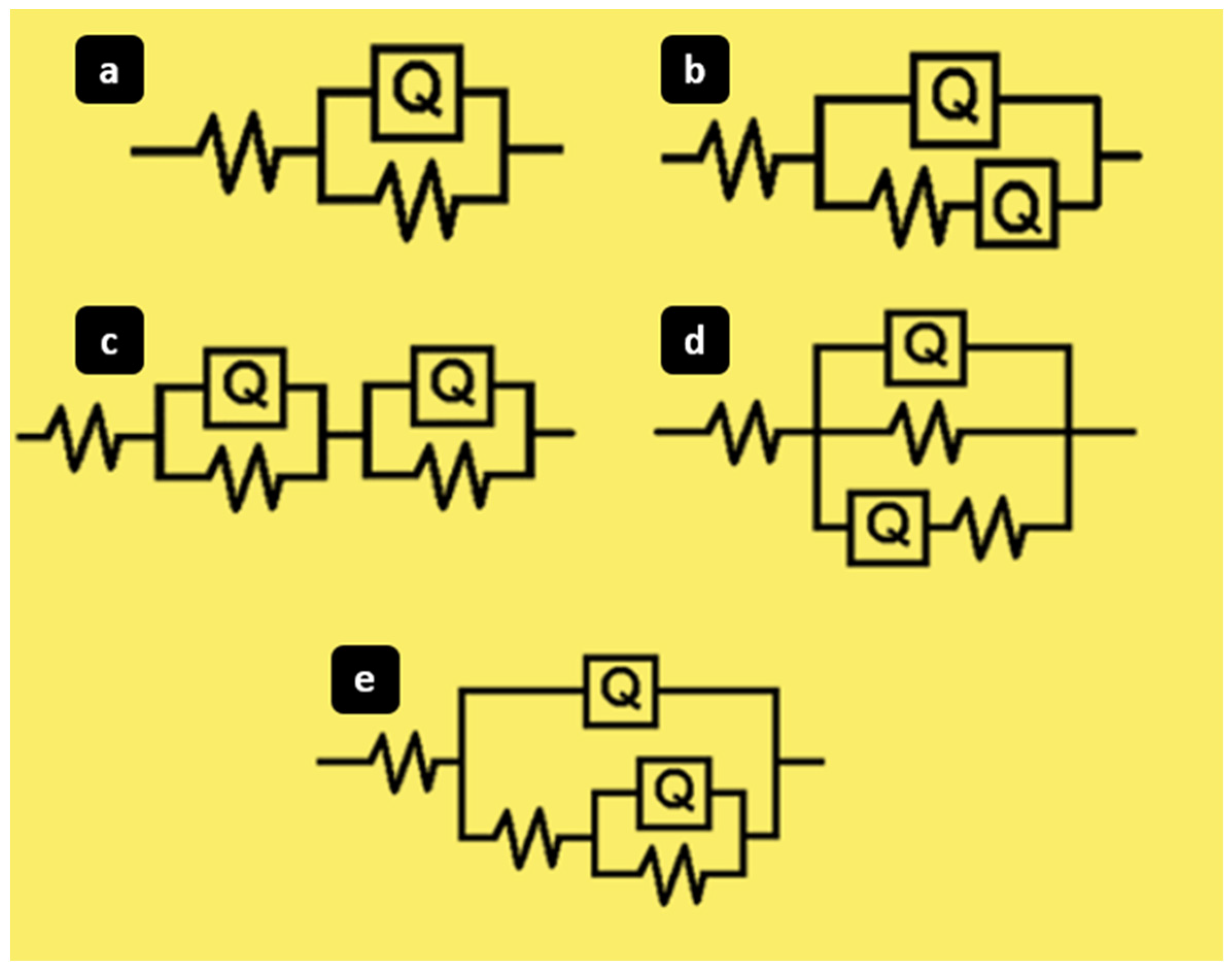
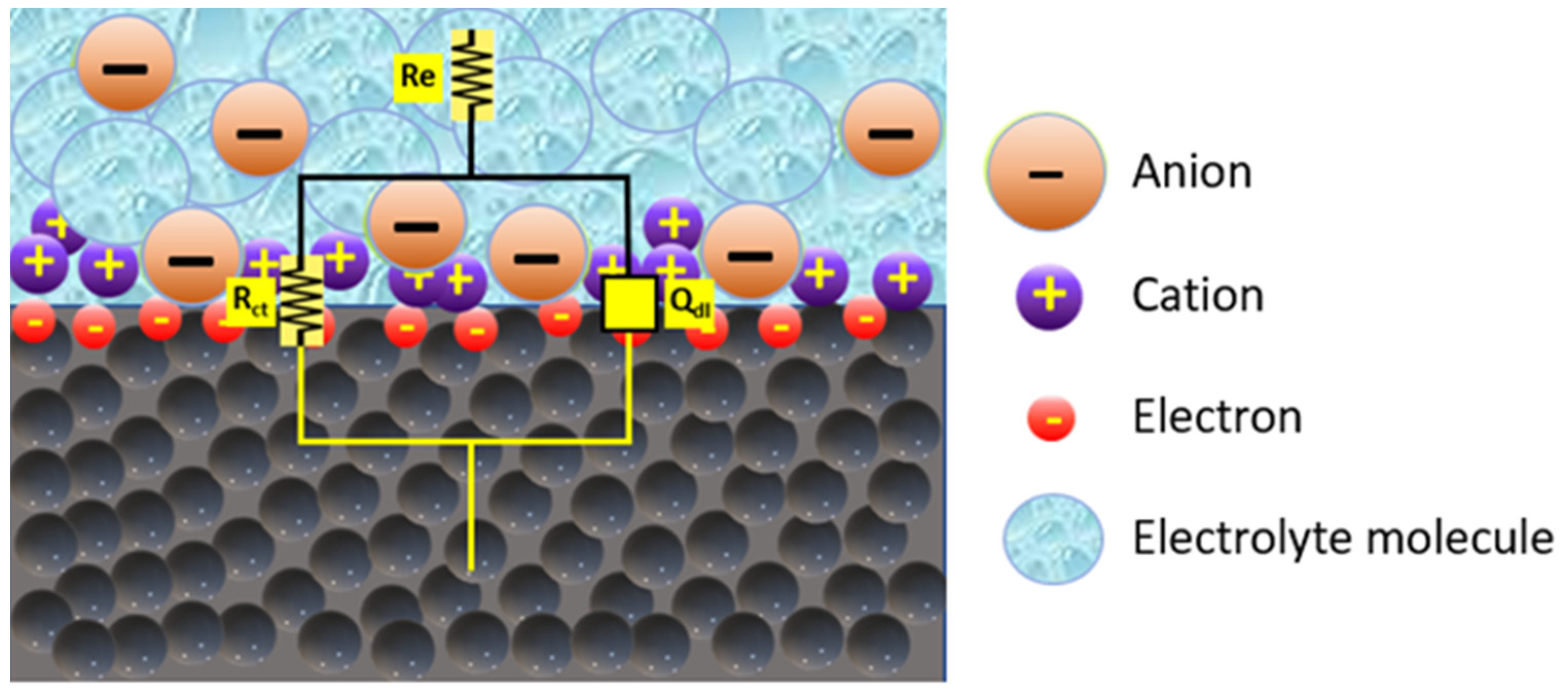
3.3. Selection of an Equivalent Electrical Circuit Model

Choosing the right equivalent circuit is of utmost importance when analyzing EIS data. The selected circuit should have a clear physical interpretation and relevance to the electrochemical system under investigation. Simplicity is key, as the circuit should capture the essential characteristics of the system without unnecessary complexity. Including too many circuit elements can lead to overfitting, which hinders accurate model predictions and complicates the interpretation of fitted parameters.

An effective equivalent circuit should provide a good fit to the experimental data. The quality of the fit can be assessed by calculating the root mean square error, which measures the deviation between the experimental data and the model predictions. By minimizing the root mean square error, the circuit can be optimized to accurately represent the electrochemical system and provide meaningful insights into its behavior.

Choosing an equivalent electrical circuit to fit experimental data in EIS involves a systematic approach. The first step is to gain a comprehensive understanding of the electrochemical system under investigation, including the electrode materials, electrolyte composition, and expected electrochemical processes.

This knowledge will help guide the selection of an appropriate equivalent circuit. For this reason, we will begin by considering basic circuit elements that represent the fundamental electrochemical processes observed in the system. For example, if there is expected charge transfer resistance, a resistor (R) can be used. If there is a double-layer capacitance, a capacitor (C) can be included, or better, a constant-phase element (Q) can be considered. We have tested different electrical equivalent circuits presented in Figure 10.

The first selected circuit is the simplest circuit, the Randles circuit (see Figure 11). It provides a simplified representation of the electrical behavior of an electrochemical cell or system. The Randles circuit consists of three basic elements: two resistors (R), and a capacitor (C). Each of these elements represents a specific electrical component in the electrochemical system.

In Figure 11, R_e means “electrolyte resistance”, R_ct is “charge transfer resistance”, and C_dl is “electrochemical double-layer capacitance”. The working electrode and counter electrode are the two endpoints of this circuit that receive current flowing from the counter electrode (on the upper side) to the working electrode (on the bottom side). Visually, it is obvious that the solution resistance R_e must be crossed before the current can proceed. However, there are two conceivable directions for the current to travel after passing through R_e. Because the current always chooses the path of least resistance, or lowest impedance, it can pass via the capacitor related with the electrochemical double-layer C_dl (the high-frequency path) or it can move through the resistor associated with charge transfer R_ct (the low-frequency path). In this instance, the frequency affects the impedance of C_dl and R_ct.

According to Kirchhoff’s circuit principles, the combined impedance of two elements in series (Re noted Z₁ and the parallel combination of R_ct and C_dl noted with Z₂) is equal to the sum of the two impedances:

$${\mathrm{Z}}_{\mathrm{series}}={\mathrm{Z}}_1+{\mathrm{Z}}_2$$

(1)

On the other hand, according to Equation (2), the inverse of the combined impedance of two parallel circuit elements is equal to the sum of the inverses of each impedance.

$$\frac{1}{{\mathrm{Z}}_{\mathrm{parallel}}}=\frac{1}{{\mathrm{Z}}_1}+\frac{1}{{\mathrm{Z}}_2}$$

(2)

Equation (2) can be arranged to form the following relation:

$${\mathrm{Z}}_{\mathrm{parallel}}=\frac{{\mathrm{Z}}_1{\mathrm{Z}}_2}{{\mathrm{Z}}_1+{\mathrm{Z}}_2}$$

(3)

As a result, by substituting each circuit component and combining them in accordance with Equation (1) through Equation (3), the total impedance of our Randles circuit (Figure 8) may be determined.

$${\mathrm{Z}}_{\mathrm{circuit}1}={\mathrm{R}}_{\mathrm{e}}+\frac{{\mathrm{Z}}_{{\mathrm{C}}_{\mathrm{dl}}}{\mathrm{Z}}_{{\mathrm{R}}_{\mathrm{ct}}}}{{\mathrm{Z}}_{{\mathrm{C}}_{\mathrm{dl}}}+{\mathrm{Z}}_{{\mathrm{R}}_{\mathrm{ct}}}}$$

(4)

Taking into account that Z_R = R and Z_C = 1/(jwC), where w is the frequency and j indicate the imaginary number (−1)^1/2, Equation (5) is obtained by substituting the corresponding impedance equations for each circuit component.

$${\mathrm{Z}}_{\mathrm{circuit}1}={\mathrm{R}}_{\mathrm{e}}+\frac{\frac{{\mathrm{R}}_{\mathrm{ct}}}{{\mathrm{jwC}}_{\mathrm{dl}}}}{{\mathrm{R}}_{\mathrm{ct}}+\frac{1}{{\mathrm{jwC}}_{\mathrm{dl}}}}$$

(5)

The total impedance of our electrochemical circuit is, thus, given in Equation (6) after reorganization and simplification.

$${\mathrm{Z}}_{\mathrm{circuit}1}={\mathrm{R}}_{\mathrm{e}}+\frac{{\mathrm{R}}_{\mathrm{ct}}}{1+{\mathrm{R}}_{\mathrm{ct}}{\mathrm{C}}_{\mathrm{dl}}\left(\mathrm{jw}\right)}$$

(6)

The denominator of Equation (6) enlarges and the proportion becomes closer to zero when w is large or w →∞. This results in Z = R_e. At the highest frequencies (1 MHz–100 kHz), it can sometimes be assumed that the impedance is identical to the solution resistance R_e, even though there is no potentiostat that can apply a frequency so high. The solution resistance must be crossed by the current at high frequencies, but it will do so via C_dl rather than R_ct. This is due to the fact that, theoretically, the capacitor’s impedance lowers as w grows (recall the equation for a capacitor’s impedance, Equation (7)). As a result, the capacitor becomes the path of least resistance at high frequencies.

$${\mathrm{Z}}_{\mathrm{c}}=\frac{1}{\mathrm{jwC}}=\frac{-\mathrm{j}}{\mathrm{wC}}$$

(7)

Analyzing the impedance data and looking for additional features that are not adequately captured by the basic circuit elements, a constant-phase element (CPE) has been chosen instead of the capacitor C_dl in order to be able to take into consideration the passivated surface’s heterogeneities. A CPE’s impedance is provided by [18]:

$${\mathrm{Z}}_{\mathrm{CPE}}=\frac{1}{{\mathrm{Y}}^0{\left(\mathrm{jw}\right)}^{\mathrm{n}}}$$

(8)

The coefficient of ideality, or “n”, is one of the characteristics acquired when modeling the system and the response of the real system is closer to the ideal as the value of n is closer to the unit and the surface is more homogeneous. Consequently, the CPE element becomes a simple resistance for n = 0 and a capacitor with capacitance Y⁰ for n = 1.

We began fitting the experimental data with the selected circuit elements using the specialized software and comparing the simulated impedance with the experimental data, which can assess the quality of the fit. We adjusted the circuit elements as needed and repeated the fitting process until a satisfactory match between the simulated and experimental data was achieved, and the results are presented in

Table 2. Circuit parameters calculated from the fitting of the EIS spectra till 0 V vs. SCE with the circuit from Figure 8 for Sample 1.

V	Re	Y/CPE	n/CPE	Rct
(Volt)	(Ω·cm2)	(S·sn/cm2)	-	(Ω·cm2)
−1.0	8.36	8.900 × 10−5	0.7624	1.87 × 105
−0.8	7.36	8.996 × 10−5	0.7415	1.73 × 104
−0.6	7.93	5.747 × 10−5	0.7981	1.33 × 104
−0.4	7.39	3.321 × 10−5	0.8135	2.89 × 104
−0.2	7.77	2.201 × 10−5	0.8657	6.87 × 104
0.0	7.55	1.394 × 10−5	0.8787	1.64 × 105

and

Table 3. Circuit parameters calculated from the fitting of the EIS spectra till 0 V vs. SCE with the circuit from Figure 8 for Sample 2.

V	Re	Y/CPE	n/CPE	Rct
(Volt)	(Ω·cm2)	(S·sn/cm2)	-	(Ω·cm2)
−1.0	9.90	8.469 × 10−5	0.7838	1.93 × 103
−0.8	9.76	6.961 × 10−5	0.7933	1.78 × 104
−0.6	9.73	5.460 × 10−5	0.5046	1.61 × 104
−0.4	9.21	3.318 × 10−5	0.8051	3.69 × 104
−0.2	9.45	2.072 × 10−5	0.8528	7.59 × 104
0.0	9.29	1.246 × 10−5	0.8699	1.24 × 105

.

A circuit with two time constants that takes into account the structure of the passive layer already formed on the surface of the materials has been employed because the single circuit has unacceptable setting errors for potentials higher than the corrosion potential. It should be kept in mind that the primary goal of this study is to determine whether the EIS technique is appropriate for this kind of system. As a result, the choice of equivalent circuit is not as crucial as the fact that it reveals whether variations in the material’s electrochemical behavior exist depending on the applied passivation potential or the material’s composition. In these instances, we have tested all of the circuits shown in Figure 10 and the provided circuit in Figure 10e and in Figure 12 is the one that most closely matches the experimental results.

The component elements are:

• R_e—electrolyte resistance;
• Q_ext—the CPE of the porous external passive layer;
• R_ext—resistance of the external porous layer;
• Q_inn—CPE of the inner passive layer;
• R_inn—resistance of the inner passive layer.

Applying the Kirchhoff’s circuit laws for this new circuit enable us to obtain:

$${\mathrm{Z}}_{\mathrm{circuit}2}={\mathrm{R}}_{\mathrm{e}}+\frac{1}{{\mathrm{jwC}}_{\mathrm{ext}}+\frac{1}{{\mathrm{R}}_{\mathrm{ext}}+\frac{1}{\frac{1}{{\mathrm{R}}_{\mathrm{int}}}+{\mathrm{jwC}}_{\mathrm{int}}}}}$$

(9)

The parameter R_e, which measures electrolyte resistance and ranges in value from 7.28 to 8.36 Ω·cm² for Sample 1 and from 9.12 to 9.94 Ω·cm² for Sample 2, displays no notable variation during the studies, indicating that no ions were discharged into the solution within the passive potential range.

The outer porous film exhibits lower resistance than the inner barrier layer, as shown by the fact that R_ext values are lower than R_inn values (see Figure 13a,b). The presence of high R_inn values at all potentials, as well as a decrease with Zr-addition, even support the establishment of a passive layer with excellent corrosion protection.

The relations between the constant-phase element (CPE, in terms of Q), the capacitance, and the thickness of the oxide film [25] are:

$$\mathrm{C}=\mathrm{gQ}{\left({\mathsf{\rho }\mathsf{\epsilon }\mathsf{\epsilon }}_0\right)}^{1-\mathrm{n}}$$

(10)

$$\mathrm{d}=\frac{{\mathsf{\epsilon }\mathsf{\epsilon }}_0\mathrm{S}}{\mathrm{C}}$$

(11)

where g is a parameter equal to 1 + 2.88(1 − n)^2.375, ρ is the electrical resistivity, ε and ε₀ represent the dielectric constant of the oxide film and the permittivity of free space, respectively; and S is the effective area of the oxide film, which is about three times the geometric area [26].

It can be observed that the protective oxide film’s thickness decreased within potential range because it can be seen that the fitted values of CPE magnitude is increasing (see Figure 13c,d).

At potentials higher than +0.6V, to obtain a better quality of the fitting process, a Warburg element was introduced into the circuit [27]. The Warburg element represents the movement/diffusion of electrons/ions in solid or liquid phases and its impedance is:

$${\mathrm{Z}}_{\mathrm{W}}=\frac{\mathrm{W}}{{\left(\mathrm{jw}\right)}^{0.5}}$$

(12)

where W is the Warburg coefficient and has the unit Ω/s^1/2.

The Warburg element at 0.8 V vs. SCE is almost 10 times higher for Sample 2 (1.09·10⁻⁴ S-sec^0.5/cm²) in comparison with this element of Sample 1 (1.17·10⁻⁵ S-sec^0.5/cm²). A higher value of the Warburg element suggests that the diffusion process is slower, which could be due to a longer diffusion path. If the diffusion path length is increased, for example, due to the presence of a thicker electrode or a more complex electrode structure, it can lead to slower diffusion and an elevated Warburg element value. Another factor to consider is the lower concentration of species: if the concentration of the diffusing species is lower, it can result in slower diffusion rates and a higher Warburg element value. The EDS [22] and XPS results [28] indicate that the passive film mainly consists of Cr₂O₃ and MoO₃, and both Cr and Mo are found in lower concentrations in Sample 2 than in Sample 1 and, thus, can explain the difference between the Warburg element values for the two samples analyzed.

4. Conclusions

In the present work, high-entropy alloys CoCrFeMoNi and Zr-doped CoCrFeMoNi were prepared using vacuum arc remelting. Electrochemical impedance spectroscopy (EIS) measurements were performed in order to select the proper electrical equivalent circuit for the prediction of the behavior of two high-entropy alloys at different potentials in artificial seawater because choosing the right equivalent circuit is of outmost importance when analyzing EIS data.

By fitting the circuit frequency response to the experimental data, circuit models with various levels of complexity and for various potential ranges were proposed and their compatibility with the experimental data was assessed. Simple electrical components were used to mimic fundamental processes, such as charge transport in bulk solutions, diffusion at low frequencies, and the development of double-layer charges at high frequencies. Additionally, it was demonstrated that various components might be used to express electrochemical events. Depending on how the parameters defining its impedance are chosen, a constant-phase element (CPE) might be used to depict both the diffusion process and the double-layer effect.

Till corrosion potential in the experimental data can be well simulated with a simple Randles circuit displaying a highly accurate fit. After this potential, the electrochemical reaction taking place at the interface between the electrolyte and the alloy involves a two-step mechanism and a proper equivalent electrical circuit was selected.

The electrolyte resistance during the experiments, for both alloys, shows no notable variation, indicating that no ions were discharged into the solution within the passive potential range. The Zr-doped high-entropy alloy sample experiences pitting corrosion over 0.20 V vs. SCE. The preferential solubility of iron ions into the electrolyte caused by the rise in the Fe segregation ratio when the high-entropy alloy is doped with Zr can be used to explain the pitting corrosion in the HEAZr alloy. At potentials higher than +0.6V, to obtain a better quality of the fitting process, a Warburg element was introduced into the circuit suggesting that the diffusion process became important.

It is important to note that selecting an equivalent circuit is often an iterative and subjective process, as it involves a balance between model complexity and the ability to accurately represent the system’s behavior. Additionally, the choice of circuit elements may vary depending on the specific electrochemical system and the phenomena of interest.

References

1. Barsoukov, E.; Macdonald, J.R. (Eds.) Impedance Spectroscopy: Theory, Experiment, and Applications; John Wiley &Sons, Inc.: Hoboken, NJ, USA, 2005. [Google Scholar] [CrossRef]
2. Socorro-Perdomo, P.P.; Florido-Suárez, N.R.; Mirza-Rosca, J.C.; Saceleanu, M.V. EIS Characterization of Ti Alloys in Relation to Alloying Additions of Ta. Materials 2022, 15, 476. [Google Scholar] [CrossRef] [PubMed]
3. López Ríos, M.; Socorro Perdomo, P.P.; Voiculescu, I.; Geanta, V.; Crăciun, V.; Boerasu, I.; Mirza Rosca, J.C. Effects of nickel content on the microstructure, microhardness and corrosion behavior of high-entropy AlCoCrFeNix alloys. Sci. Rep. 2020, 10, 21119. [Google Scholar] [CrossRef]
4. Jimenez-Marcos, C.; Mirza-Rosca, J.C.; Baltatu, M.S.; Vizureanu, P. Experimental Research on New Developed Titanium Alloys for Biomedical Applications. Bioengineering 2022, 9, 686. [Google Scholar] [CrossRef]
5. Avram, D.N.; Davidescu, C.M.; Dan, M.L.; Mirza-Rosca, J.C.; Hulka, I.; Pascu, A.; Stanciu, E.M. Electrochemical Evaluation of Protective Coatings with Ti Additions on Mild Steel Substrate with Potential Application for PEM Fuel Cells. Materials 2022, 15, 5364. [Google Scholar] [CrossRef] [PubMed]
6. Avram, D.N.; Davidescu, C.M.; Dan, M.L.; Mirza-Rosca, J.C.; Hulka, I.; Stanciu, E.M.; Pascu, A. Corrosion resistance of NiCr(Ti) coatings for metallic bipolar plates. Mater. Today Proc. 2023, 72, 538–543. [Google Scholar] [CrossRef]
7. Avram, D.N.; Davidescu, C.M.; Dan, M.L.; Stanciu, E.M.; Pascu, A.; Mirza-Rosca, J.C.; Iosif, H. Influence of titanium additions on the electrochemical behaviour of nicr/ti laser cladded coatings. Ann. Dunarea Jos Univ. Galati Fascicle XII Weld. Equip. Technol. 2022, 33, 107–111. [Google Scholar] [CrossRef]
8. Perdomo-Socorro, P.P.; Florido-Suárez, N.R.; Verdú-Vázquez, A.; Mirza-Rosca, J.C. Comparative EIS study of titanium-based materials in high corrosive environments. Int. J. Surf. Sci. Eng. 2021, 15, 152–164. [Google Scholar] [CrossRef]
9. Arabzadeh, H.; Shahidi, M.; Foroughi, M.M. Electrodeposited polypyrrole coatings on mild steel: Modeling the EIS data with a new equivalent circuit and the influence of scan rate and cycle number on the corrosion protection. J. Electroanal. Chem. 2017, 807, 162–173. [Google Scholar] [CrossRef]
10. Lopez-Dominguez, D.; Gomez-Guzman, N.B.; Porcayo-Calderón, J.; Lopez-Sesenes, R.; Larios-Galvez, A.K.; Sarmiento-Bustos, E.; Rodriguez-Clemente, E.; Gonzalez-Rodriguez, J.G. An Electrochemical Study of the Corrosion Behaviour of T91 Steel in Molten Nitrates. Metals 2023, 13, 502. [Google Scholar] [CrossRef]
11. Larios-Galvez, A.K.; Vazquez-Velez, E.; Martinez-Valencia, H.; Gonzalez-Rodriguez, J.G. Effect of Plasma Nitriding and Oxidation on the Corrosion Resistance of 304 Stainless Steel in LiBr/H2O and CaCl2-LiBr-LiNO3-H2O Mixtures. Metals 2023, 13, 920. [Google Scholar] [CrossRef]
12. Revilla, R.I.; Wouters, B.; Andreatta, F.; Lanzutti, A.; Fedrizzi, L.; De Graeve, I. EIS comparative study and critical Equivalent Electrical Circuit (EEC) analysis of the native oxide layer of additive manufactured and wrought 316L stainless steel. Corros. Sci. 2020, 167, 108480. [Google Scholar] [CrossRef]
13. Zhao, Z.; Zou, Y.; Liu, P.; Lai, Z.; Wen, L.; Jin, Y. EIS equivalent circuit model prediction using interpretable machine learning and parameter identification using global optimization algorithms. Electrochim. Acta 2022, 418, 140350. [Google Scholar] [CrossRef]
14. Martinez, S.; Šoić, I.; Špada, V. Unified equivalent circuit of dielectric permittivity and porous coating formalisms for EIS probing of thick industrial grade coatings. Prog. Org. Coat. 2021, 153. [Google Scholar] [CrossRef]
15. Diard, J.P.; Montella, C. Non-intuitive features of equivalent circuits for analysis of EIS data. The example of EE reaction. J. Electroanal. Chem. 2014, 735, 99–110. [Google Scholar] [CrossRef]
16. Scully, J.; Silverman, D.; Kendig, M. (Eds.) Electrochemical Impedance: Analysis and Interpretation; ASTM International: West Conshohocken, PA, USA, 1993; ISBN 978-0-8031-1861-4. [Google Scholar]
17. Wang, S.; Zhang, J.; Gharbi, O.; Vivier, V.; Gao, M.; Orazem, M.E. Electrochemical impedance spectroscopy. Nat. Rev. Methods Prim. 2021, 1, 41. [Google Scholar] [CrossRef]
18. Boukamp, B.A. A Nonlinear Least Squares Fit procedure for analysis of immittance data of electrochemical systems. Solid State Ion. 1986, 20, 31–44. [Google Scholar] [CrossRef] [Green Version]
19. Material, C.; Databases, P. Standard Reference Test Method for Making Potentiostatic and Potentiodynamic Anodic. Annu. B ASTM Stand. 2004, 94, 1–12. [Google Scholar]
20. ASTM Standard G102-89; Standard Practice for Calculation of Corrosion Rates and Related Information from Electrochemical Measurements. ASTM International: West Conshohocken, PA, USA, 2006.
21. ISO 16773-1-4:2016; Electrochemical Impedance Spectroscopy (EIS) on Coated and Uncoated Metallic Specimens. International Organization for Standardization: Geneva, Switzerland, 2016.
22. Brito-Garcia, S.; Mirza-Rosca, J.; Geanta, V.; Voiculescu, I. Mechanical and Corrosion Behavior of Zr-Doped High-Entropy Alloy from CoCrFeMoNi System. Materials 2023, 16, 1832. [Google Scholar] [CrossRef]
23. Wang, Z.; Feng, Z.; Zhang, L. Effect of high temperature on the corrosion behavior and passive film composition of 316 L stainless steel in high H2S-containing environments. Corros. Sci. 2020, 174, 108844. [Google Scholar] [CrossRef]
24. Wang, Z.; Zhang, L.; Zhang, Z.; Lu, M. Combined effect of pH and H2S on the structure of passive film formed on type 316L stainless steel. Appl. Surf. Sci. 2018, 458, 686–699. [Google Scholar] [CrossRef]
25. Orazem, M.E.; Frateur, I.; Tribollet, B.; Vivier, V.; Marcelin, S.; Pébère, N.; Bunge, A.L.; White, E.A.; Riemer, D.P.; Musiani, M. Dielectric Properties of Materials Showing Constant-Phase-Element (CPE) Impedance Response. J. Electrochem. Soc. 2013, 160, C215–C225. [Google Scholar] [CrossRef] [Green Version]
26. Kocijan, A.; Merl, D.K.; Jenko, M. The corrosion behaviour of austenitic and duplex stainless steels in artificial saliva with the addition of fluoride. Corros. Sci. 2011, 53, 776–783. [Google Scholar] [CrossRef]
27. Jáquez-Muñoz, J.M.; Gaona-Tiburcio, C.; Méndez-Ramírez, C.T.; Baltazar-Zamora, M.Á.; Estupinán-López, F.; Bautista-Margulis, R.G.; Cuevas-Rodríguez, J.; Flores-De los Rios, J.P.; Almeraya-Calderón, F. Corrosion of Titanium Alloys Anodized Using Electrochemical Techniques. Metals 2023, 13, 476. [Google Scholar] [CrossRef]
28. Wang, W.; Wang, J.; Sun, Z.; Li, J.; Li, L.; Song, X.; Wen, X.; Xie, L.; Yang, X. Effect of Mo and aging temperature on corrosion behavior of (CoCrFeNi)100-xMox high-entropy alloys. J. Alloys Compd. 2020, 812, 152139. [Google Scholar] [CrossRef]
Figure 1. Sample obtention and preparation for the tests.
Metals 13 01204 g001
Figure 2. Images obtained by optical microscopy showing the microstructure of the samples.
Metals 13 01204 g002
Figure 3. SEM micrographs, EDS spectra, and composition for Sample 1 (a) and Sample 2 (b).
Metals 13 01204 g003
Figure 4. Open-circuit corrosion potential diagrams of Samples 1 and 2.
Metals 13 01204 g004
Figure 5. Linear polarization curves of the analyzed samples.
Metals 13 01204 g005
Figure 6. After corrosion, SEM micrographs, EDS spectra, and composition for Sample 1 (a) and Sample 2 (b).
Metals 13 01204 g006
Figure 7. Nyquist plots of Sample 1 and Sample 2.
Metals 13 01204 g007
Figure 8. Bode-phase plots of Sample 1 (a,b) and Sample 2 (c,d).
Metals 13 01204 g008
Figure 9. Bode |Z| plots of Sample 1 and Sample 2 at negative potentials (a,c) and positive potentials (b,d).
Metals 13 01204 g009
Figure 10. Different electrical equivalent circuits used for fitting the experimental data: (a) R(QR), (b) R(Q(RQ)), (c) R(QR)(RQ), (d) R(QR(QR)), and (e) R(Q(R(QR))).
Metals 13 01204 g010
Figure 11. Randles circuit used to fit the experimental data.
Metals 13 01204 g011
Figure 12. The second electrical equivalent circuit used for EIS data simulation.
Metals 13 01204 g012
Figure 13. Electrical-circuit parameters: resistance of the inner layer (a) and external layer (b), and the CPE magnitude for the inner layer (c) and external layer (d).
Metals 13 01204 g013