Review

The Paramagnetic Meissner Effect (PME) in Metallic Superconductors

by
Michael Rudolf Koblischka
1,*,
Ladislav Půst
2,
Crosby-Soon Chang
3,4,
Thomas Hauet
3 and
Anjela Koblischka-Veneva
1
1
Saarland University, P.O. Box 151150, 66041 Saarbrücken, Germany
2
ELI Beamlines Facility, The Extreme Light Infrastructure ERIC, Za Radnicí 835, 25241 Dolní Břežany, Czech Republic
3
Institut Jean Lamour, UMR CNRS-Université de Lorraine, 54506 Vandœvre-lès-Nancy, France
4
Sheridan Institute of Higher Education, Piccadilly Square West Building, 18/7 Aberdeen St, Perth, WA 6000, Australia
*
Author to whom correspondence should be addressed.
Metals 2023, 13(6), 1140; https://doi.org/10.3390/met13061140
Submission received: 30 April 2023 / Revised: 5 June 2023 / Accepted: 10 June 2023 / Published: 19 June 2023

Abstract

:
The experimental data in the literature concerning the Paramagnetic Meissner Effect (PME) or also called Wohlleben effect are reviewed with the emphasis on the PME exhibited by metallic, s-wave superconductors. The PME was observed in field-cool cooling (FC-C) and field-cool warming (FC-W) m ( T ) -measurements on Al, Nb, Pb, Ta, in compounds such as, e.g., NbSe 2 , In-Sn, ZrB 12 , and others, and also in MgB 2 , the metallic superconductor with the highest transition temperature. Furthermore, samples with different shapes such as crystals, polycrystals, thin films, bi- and multilayers, nanocomposites, nanowires, mesoscopic objects, and porous materials exhibited the PME. The characteristic features of the PME, found mainly in Nb disks, such as the characteristic temperatures T 1 and T p and the apparative details of the various magnetic measurement techniques applied to observe the PME, are discussed. We also show that PME can be observed with the magnetic field applied parallel and perpendicular to the sample surface, that PME can be removed by abrading the sample surface, and that PME can be introduced or enhanced by irradiation processes. The PME can be observed as well in magnetization loops (MHLs, m ( H ) ) in a narrow temperature window T p < T c , which enables the construction of a phase diagram for a superconducting sample exhibiting the PME. We found that the Nb disks still exhibit the PME after more than 20 years, and we present the efforts of magnetic imaging techniques (scanning SQUID microscopy, magneto-optics, diamond nitrogen-vacancy (NV)-center magnetometry, and low-energy muon spin spectroscopy, (LE- μ SR)). Various attempts to explain PME behavior are discussed in detail. In particular, magnetic measurements of mesoscopic Al disks brought out important details employing the models of a giant vortex state and flux compression. Thus, we consider these approaches and demagnetization effects as the base to understand the formation of the paramagnetic signals in most of the materials investigated. New developments and novel directions for further experimental and theoretical analysis are also outlined.

1. Introduction

The superconducting state is characterized by two hallmarks: the vanishing electrical resistance below the superconducting transition temperature, T c , and the Meissner–Ochsenfeld effect [1], describing the expulsion of magnetic flux from the superconducting sample when cooling it in an applied magnetic field (field cooling, FC), creating a diamagnetic state with negative magnetization, m. This implies that the induced screening currents try to expel the magnetic flux from the sample. The implications of the Meissner–Ochsenfeld effect led directly to the development of the basic theories of superconductivity (London, Ginzburg–Landau, and BCS), and are intensively described in all textbooks on superconductivity (see, e.g., [2,3,4,5,6,7,8,9,10]). Thus, the first observations of superconducting transitions of Bi-based, high- T c superconductors (HTSc) to a paramagnetic state (positive magnetization, m, attracting magnetic field) instead of a diamagnetic one were more treated as experimental mishaps and went mostly unnoticed by the community [11,12]. The situation changed with more detailed measurements on granular Bi 2 Sr 2 CaCu 2 O 8 (Bi-2212) samples by Braunisch et al. [13,14], linking the observation of a superconducting transition in field-cooling m ( T ) -curves towards the paramagnetic state with unique features of the HTSc, i.e., the so-called d-wave superconductivity and effects of granularity ( π -junctions between the grains). This was soon followed by other researchers, applying also different measurement techniques to exclude possible experimental artifacts and providing some theories to explain these observations [15,16,17,18,19,20,21,22,23,24]. Following these works, several theoretical approaches were published concerning this effect, now named paramagnetic Meissner effect (PME) or Wohlleben effect [18]. The key element of the PME is thus the observation of positive magnetization upon field-cool cooling (FC-C) or warming (FC-W) in m ( T ) -measurements.
Thus, it came as a big surprise as Thompson et al. presented an observation of PME on bulk niobium disks, a classical s-wave superconductor [25,26], or often called conventional or low- T c superconductor (LTSc). This work was soon followed by Kostić et al. presenting a thorough investigation of the PME in Nb materials [27]. This work resulted in a comment [28] and a reply [29], where the inherent differences between the PME in metallic, s-wave superconductors and the HTSc (d-wave superconductors) were clarified. Furthermore, several reports presented details of the superconducting transitions on different Nb samples with the magnetic field applied in parallel and perpendicular directions [26,30], the vanishing of the PME by surface treatments [27,31], and the enhancement of the PME by ion implantantion [32]. In this way, a new research direction was born.
The mostly isotropic LTSc used for these studies were compact, bulk, and homogeneous materials in stark contrast to HTSc, which are typically granular materials with their inherent complicated crystal structures, mostly tetragonal ones. Therefore, the LTSc may serve—owing to their relative simplicity—as a superconducting model system to perform detailed studies in order to clarify the physical origin of the paramagnetic moment appearing when crossing through T c from higher temperatures.
Since then, the PME was observed in a variety of metallic superconductors [33,34,35,36,37,38,39,40,41,42,43,44,45,46,47,48], and in different forms such as thin films [49,50,51,52], nanowire arrays [53], multilayer systems [54,55,56,57,58,59], and very importantly, in nanocomposites [60,61] and mesoscopic structured samples [62,63,64,65,66]. Multilayered materials may be composed of superconductor/normal metal, but also superconducting/para- or ferromagnetic ones. Of course, since the discovery of MgB 2 —the metallic superconductor with the highest transition temperature [67,68]—it was only a matter of time before reports of PME in this system appeared in the literature as well [69,70,71,72,73,74].
All these observations of PME involve a large variety of superconducting materials and various sample shapes. Thus, it is the aim of the present review to summarize all these experimental efforts, which will contribute to a better comprehension of the observations of the PME in metallic superconductors.
Several theoretical approaches [75,76,77,78,79,80,81,82,83,84,85,86,87,88,89,90,91,92,93,94,95,96] to explain the PME were already reviewed by Li [97], but only a short summary of the experimental data was given in this article. Here, it is important to point out that two basically different explanations for the PME exist in the literature:
(i)
Extrinsic PME. Here, the PME is not related to the material properties, but to properties of the sample surface, surface superconductivity, or the spatial variation of the superconducting properties in a given sample. This is the case for the giant vortex state [85,86], flux trapping, and compression effects [82], which will be discussed in detail later on in this review.
(ii)
Intrinsic PME. In this case, the PME is an inherent material property. The PME may be originating by the presence of Josephson coupled π junctions, which could arise due to the unconventional order parameter (e.g., the d-wave symmetry in HTSc cuprates [28,92]). Furthermore, s-wave odd-frequency superconductivity may occur in a two-band superconductor (e.g., MgB 2 , pnictides) [98,99] or in superconductor/nonsuperconductor and superconductor–magnet hybrid systems [100,101,102,103,104,105,106], where the time-reversal symmetry of the superconducting condensate is broken by magnetic ordering and thus can result in the stabilization of an odd-frequency superconducting state.
The theoretically oriented review of Li [97] could not provide a solution to the (still) ongoing discussion regarding which explanation may be the correct one, leaving this question open to new results appearing in the future. Thus, it is also not the intention of the present review to revive the discussion regarding which explanation is the correct one. Very recently, PME was also observed in superconducting boron-doped diamond thin films [107], which represents an elemental superconductor, but not a classic metallic one. Furthermore, renewed interest in superconductor/nonsuperconductor and superconductor/ferromagnetic Josephson junctions as well as in multiband superconductors led to new theoretical predictions of paramagnetic Meissner currents (intrinsic PME) in such systems. However, the experimental proof of these predictions turned out to be difficult with currently only one successful demonstration in the literature [108].
Therefore, the present review mainly focuses on the experimental observations of the PME in metallic s-wave superconductors in bulk or mesoscopic forms. We further provide new experimental results obtained since the first review article published in 2003, work out the distinct differences between the PME of HTSc superconductors and the metallic ones, and discuss the experimental difficulties for the observation of the PME.
This manuscript is organized as follows. In Section 2, we present the various experimental observations found in the literature. Section 2.1 gives an introduction to the PME found first in polycrystalline Bi-2212 HTSc samples and compares these reults to the observations of the PME on bulk Nb disks. A third type of PME was observed in YBCO thin films, patterned YBCO structures, and YBCO nanowires, which has only some features in common with the other two cases. In Section 2.2, the observations of paramagnetic signals upon field-cooling of various metallic superconductors are reviewed. Then, in Section 2.3, we discuss the various methods applied to observe PME, which is very important to understand the data published in the literature. Section 3 focuses on details of the specific experiments performed in Detroit, Tokyo, and Nancy on bulk Nb disks to elucidate the nature of the PME. Firstly, the parameters of the investigated samples are presented in Section 3.1. The measurements described in detail include the m ( T ) -behavior with PME (Section 3.2), the magnetic hysteresis loops at temperatures close to T c (Section 3.3), and discusses the experiments performed in the literature to enhance or reduce the PME (Section 3.4). Furthermore, Section 3.5 presents investigations of PME as a function of time, and Section 3.6 presents AC susceptibility measurements on the Nb disks. In Section 4, the attempts to imagine the giant vortex state and flux structures close to the superconducting transition are discussed. In Section 5, the most important models to describe the PME in the metallic superconductors are outlined. Finally, Section 6 presents the conclusions and an outlook to further investigations of the PME.

2. Experimental Data of PME

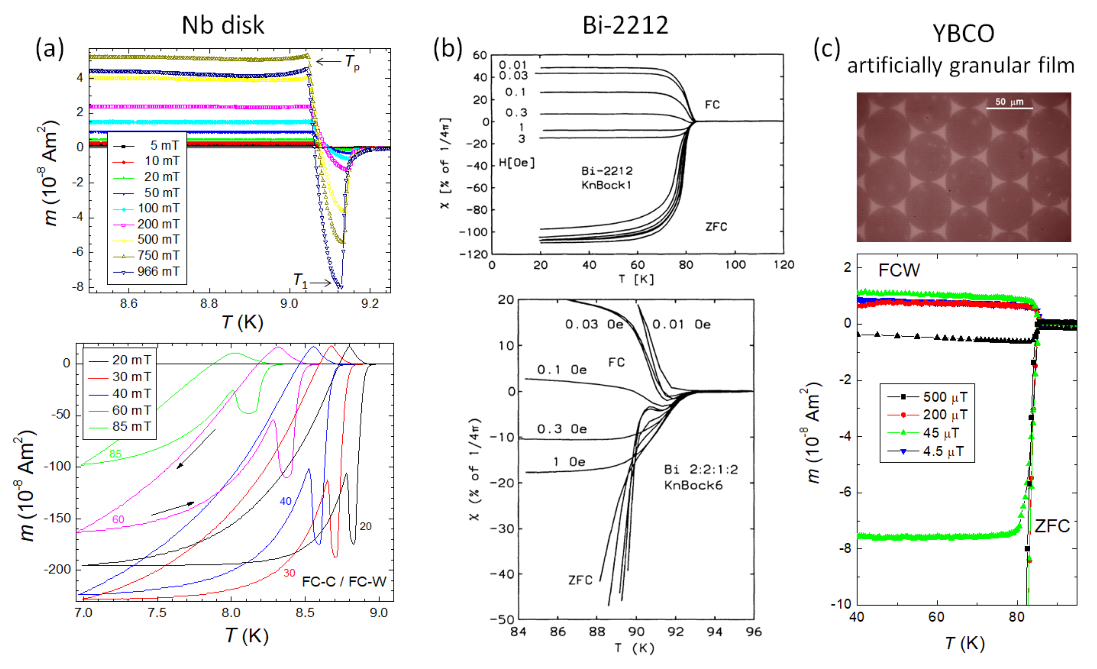
2.1. Comparison of the PME in HTSc and Metallic Superconductors

We start with a comparison of the PME found in bulk Nb disks (see Figure 1a, [26]) with that of HTSc Bi-2212 polycrystalline ceramics (see Figure 1b, [13]) and an artificially patterned YBCO thin film sample (see Figure 1c, [109,110,111]). For all three samples, the magnetization is plotted versus temperature, m ( T ) . The PME is observed when field-cooling (FC-C) or field-warming (FC-W) the sample in a small applied magnetic field. The third cooling mode is zero-field cooling (ZFC), where the sample is cooled in zero field to the lowest temperature, and then a small magnetic field is applied. In this mode, signatures of PME may also be observed (lower panel of Figure 1b). The features found in Figure 1a–c are, at first glance, qualitatively the same; in all three cases, there results a positive  m ( T ) signal, i.e., a paramagnetic signal, when cooling the sample in quite small fields, and the positive m ( T ) signal reduces gradually when applying larger magnetic fields. However, it is also quite obvious that the Nb disk exhibits very clear minima ( T 1 )/maxima ( T p ) on field cooling as well as on warming, whereas these features are less clear in Bi-2212 (Figure 1b) and practically non-existent in the case of the patterned YBCO film (Figure 1c).
In ref. [112], the authors list some more distinct differences of the PME in Nb and Bi-2212 samples: “Before proceeding to a discussion of our experiment we would like to remark that these two forms of paramagnetism in ceramic Bi-2212 and in a bulk Nb sample can be clearly distinguished in several other ways. For example, the cooling rate affects the magnetic response differently in the two cases. Recent experimental data show significant differences between Nb and granular Bi-2212 HTSc samples. While slow cooling enhances the paramagnetic signal for the granular sample, it is diminished in the Nb sample. This clearly indicates that the equilibrium state of both samples in a small magnetic field is quite different [113]. For the Nb discs Koshelev and Larkin gave an explanation based on the idea that during the cooling process the surface region nucleates superconductivity before the bulk, so that magnetic flux in the sample is compressed and creates an enhanced magnetization [82]. This compressed flux mechanism leads to a metastable state which depends on the cooling procedure whereas the polarization of the spontaneous orbital moments is an equilibrium process. Further, noise measurements of the magnetization of Bi-2212 give signals which are compatible with the presence of spontaneous orbital moments [114]”.
The more detailed measurements on the Nb disks performed in the Detroit group in the later years also revealed several important differences between the polycrystalline HTSc samples and the bulk Nb samples, such as the presence of two characteristic temperatures, T 1 and T p (see the lower panel of Figure 1a), at all applied magnetic fields, and the different shape of the magnetization loops in the temperature range between T p and T c . This will be discussed in detail in Section 3 below.
The situation of the sample in Figure 1c is completely different. This sample is patterned from a homogeneous YBa 2 Cu 3 O 7 δ (YBCO) thin film [109,110], which in its original form did not show any PME. The structure is pictured in the top graph of Figure 1c. The sample does not contain any weak links, which one expects from a granular sample, but the current paths between the individual disks are constricted to a narrow area, where the disks are touching each other. This guarantees the flow of a strong inter-disk current, but with a changed field dependence. Thus, the PME in this sample is only observed at very low applied fields, and entirely extrinsic as being caused by trapped flux between the disks. Specific features of the PME such as the characteristic temperatures T 1 and T p could not be observed here, as there is no contribution of surface superconductivity. Interestingly enough, practically the same situation was encountered recently when investigating the magnetic properties of superconducting YBCO nanofiber mats [115,116], where the supercurrents can flow in local rings as well. Thus, the resulting PME signals resemble the ones of this artificially granular thin film, but with a much smaller signal strength as compared to the thin film sample.
In the literature, there is a fourth type of PME reported, the so-called high-field PME or HFPME [117,118,119], which is only observed on HTSc bulk samples of the (RE)BCO-type (where RE = Y, Nd, Eu, Sm, Gd) when measuring superconducting transitions in high applied magnetic fields. The m ( T ) -signals recorded first go to negative values at T c , but then start to turn towards positive values at lower temperatures. However, the recorded transitions are fully different from the ones of polycrystalline Bi-2212 [13,14], which suggest a different origin. In refs. [120,121], we could show that the superconducting transition may be only a small negative contribution to an otherwise positive m ( T ) -signal when measuring various (RE)BCO bulk superconductors, including GdBCO, NdBCO, or a mixture such as (Nd, Eu, Gd)BCO (abbreviated NEG). In particular, GdBCO may show a Néel temperature below 4 K to a ferromagnetic state. So, this high-field PME is mainly caused by such strong paramagnetic magnetic moments inherent to the sample itself.

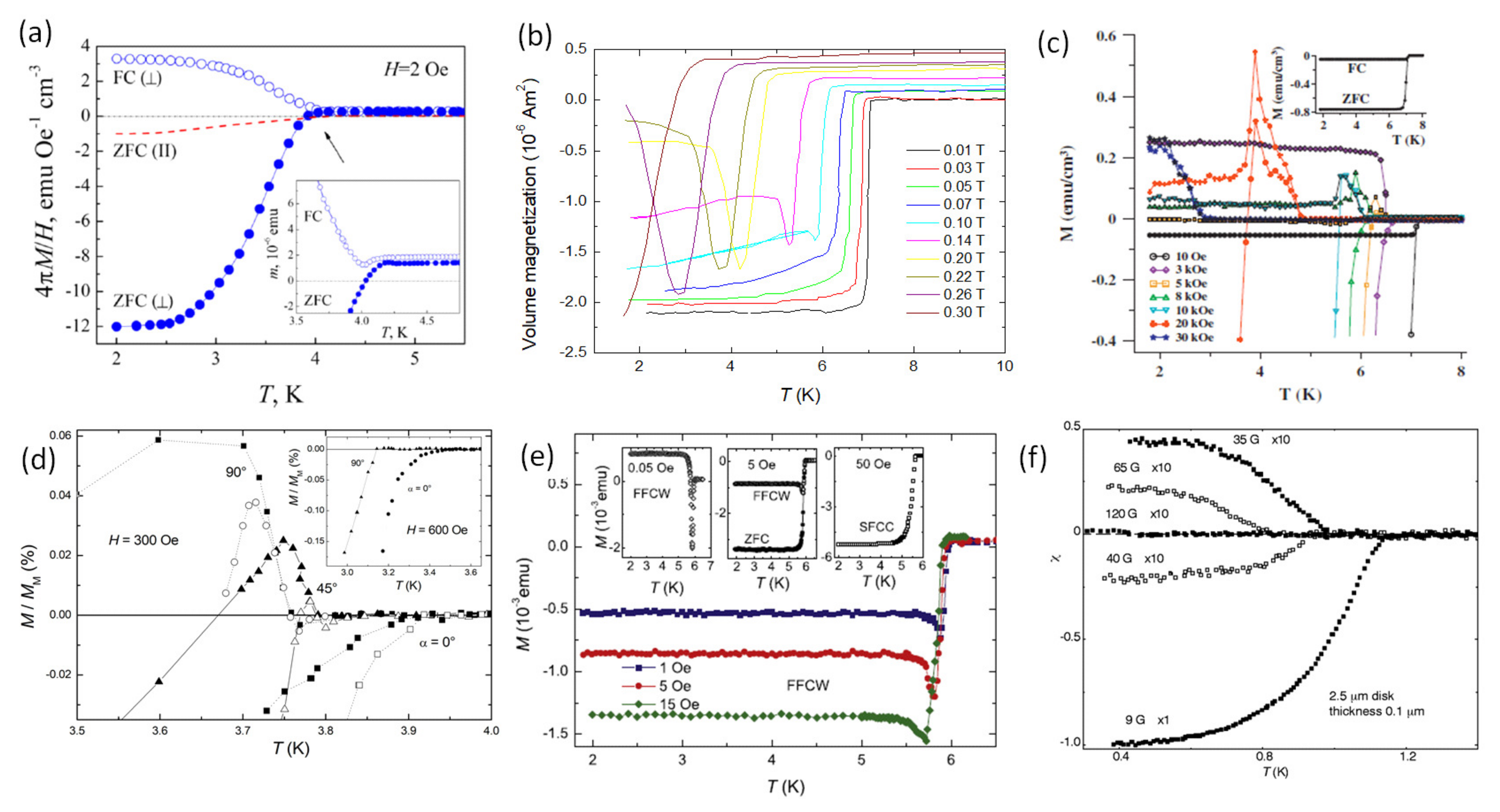
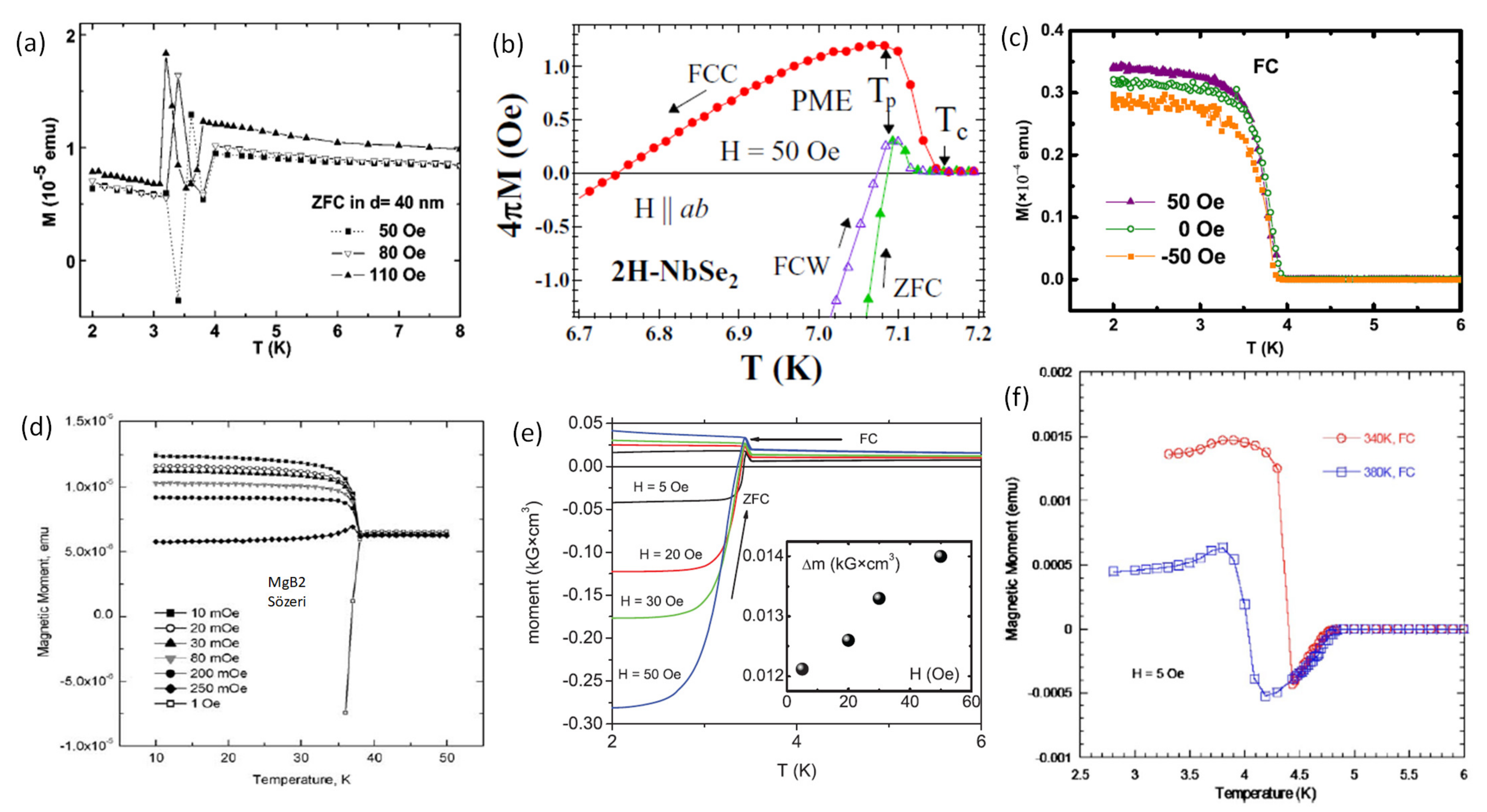
2.2. Metallic Superconducting Samples with PME

Figure 2 and Figure 3 present observations of the PME on a variety of metallic superconductors, where FC curves result in positive values of m ( T ) . In nearly all these measurements, the external magnetic field is applied perpendicular to the sample surface unless noted otherwise (Figure 2a,d and Figure 3a). This also applies to the various measurements on the Nb disks with the exception of Figure 10. However, only some of the authors also provide detailed graphs of the superconducting transition region, where some of the characteristic features, such as in the case of the Nb disks, can be seen, e.g., the work of Ramjan et al. [122] on V 0.6 Ti 0.4 alloys with varying Y-content or the measurements on SrBi 3 crystals by Zhang et al. [48]. Some of the samples investigated are even multilayers where one component may be magnetic, or samples with different amounts of additional doping, which can be either paramagnetic or ferromagnetic [54,55,56,61,108,123]. Such samples may exhibit positive (paramagnetic) m ( T ) signals in the entire temperature range also above the superconducting transition, so the magnetic signals must be worked out properly and be subtracted from the respective plot. This makes the comparison of the curves found in the literature quite difficult. On the other hand, wherever the measurements provide the details close to T c , the characteristic minima and maxima can be observed in the m ( T ) -curves, which clearly points to the importance of the two characteristic temperatures, T 1 and T p .
We further must note here that some of the experiments reported in the literature did only show the presence of PME in their specific system, but some of the experiments carried out were indeed dedicated and planned experiments to test the theoretical predictions for the occurrence of the PME, which nicely reflects that the metallic superconductors are the workhorses for experimentalists.
The PME was observed up to now on a large variety of metallic superconductors including Nb (bulk disks, bars, thin films, as well as nanostructured samples), Pb (on bulk disks, but also in nanowire arrays and Pb-porous glass nanocomposites), mesoscopic structures of Al and Nb [62], Ta, 2H-NbSe 2 single crystals, Nb-AlO x -Nb tunnel junctions, SrBi 3 and ZrB 12 single crystals with specific vortex–vortex interaction, indium-tin oxide films with electrochemical doping (e.g., Mg), Ca 3 Rh 4 Sn 13 , Ti-V alloys, Nb-Gd composite thin films, Bi 2 Te 3 -FeTe heterostructure, Mo 100 x Re x alloy, Dy 1 x Y x Rh 4 B 4 , Co/Nb multilayers, Ag/Nb proximity structures, and also the MgB 2 system [69,70,71,72,73,74], which represents the metallic superconductor with the highest transition temperature. Here, we must note that the PME in MgB 2 was always observed in polycrystalline samples (bulks or tapes), where the grain connectivity may be different depending on the chosen preparation route.
A different issue is the various superconducting/ferromagnetic compounds, which can be multilayered thin films or materials with chemical doping [54,55,56,60,61]. Here, the presence of a ferromagnetic material provides extra stray fields when cooling the sample below T c . All authors mainly discuss the field trapping/compression as the main reason for observing the PME.
Another unique case is superconducting B-doped diamond (BDD) thin film with various doping levels [107]. Such samples were reported to exhibit PME in m ( T ) -curves recorded in 1–15 mT (10–150 Oe) applied magnetic fields. BDD is a disordered s-wave superconductor and π junctions could be produced by spin-flip scattering of spin ½ moments when present at weak superconducting regions. A frustrated network of 0 and π junctions will result in a distribution of spontaneous equilibrium supercurrents, a spin glass (phase glass) state. Besides PME, the samples also showed a pressure-induced spin glass type anomaly below T c in one sample. The authors suggested that the two effects together imply the emergence of π junctions in the bulk of the BDD films, from structural inhomogeneity and spin-flip scattering mechanism.
The muon-based experiment of DiBernardo [108] represents a dedicated attempt to demonstrate the intrinsic PME (odd s-wave superconductivity) in a metal–ferromagnet hybrid system (Au-Ho-Nb trilayer), which is a non-trivial task as such hybrid systems cannot be investigated by magnetometry. These results will be discussed further in Section 4.
Figure 2a–f and Figure 3a–f give several experimental results on various metallic superconductors. Table 1 lists all PME experiments on metallic superconductors, together with the data for the superconducting transition temperature (onset), the recorded transition width Δ T c , κ , the references, and some remarks on the experiment itself. In particular, the PME observations on mesoscopic metallic superconductors (Al, Nb) [62,64] gave very important input to the understanding of the PME. The same applies to the measurements on ZrB 12 crystals with a unique vortex–vortex interaction [37], making the material an intermediate 1.5-type superconductor. This we will discuss in Section 5 in detail.
Furthermore, of course, samples of the metallic superconductors are much better suited than HTSc materials (deposition of clean thin films, patterning) to attempt the various types of magnetic imaging of the vortex structures, as we will see later in Section 4 below.
After the first observations of the PME in the Bi-2212 HTSc, the work in this direction also continued. Here, we list only some of the contributions as this could be a topic of its own, dedicated review. Even more details on the superconducting transitions of Bi-2212 were worked out [124,125], and several more types of HTScs were found to exhibit the PME, such as YBCO as thin films, polycrystalline bulks, single crystals or nanofiber mats [17,115,116,126,127,128,129], La 1 x Sr x CuO 4 [130], the electron-doped superconductor Nd 2 x Ce x CuO y [131], the bismuthate Ba 1 x K x BiO 3 [132] and RSr 2 Cu 2 NbO 7 δ compounds (R = Y, Pr, and Gd), which have a crystallographic structure like YBCO [133]. Furthermore, the PME was observed in measurements of the iron-based superconductors (IBS), such as K 0.8 Fe 1.7 Se 2 [134]. An important issue we must note here is that all these HTSc materials mentioned here are typically granular, and most of the samples studied are such with T c < 77 K. Very recently, PME measurements were carried out on an YBCO thin film with embedded BaHfO 3 nanorods, yielding m ( T ) -curves similar to the artificial granular YBCO film (see Figure 1c and YBCO nanofiber mats [135]). The authors ascribe the observation of PME due to field-trapping along the non-superconducting nanorods.
Thus, the metallic superconductors represent a large playground for the observation of the PME in clearly non-d-wave superconductors. This also applies for the measurements in MgB 2 , representing a two-band superconductor with all tunable inter-grain properties [68,136,137]. Interestingly enough, there are no observations of the PME reported in granular systems, such as metallic superconductor wires of NbTi or Nb 3 Sn, which may be a consequence of the strong coupling between the grains in these materials [7,138].
Table 1. Metallic superconductors exhibiting the PME. Given are the various materials, the sample type, the superconducting transition temperature, T c , in Kelvin, the transition width, Δ T c , the Ginzburg–Landau parameter κ , the respective citations, and some remarks on the experiment. The abbreviation nps denotes nanoparticles, ⌀ stands for diameter, and ITO = Indium Tin Oxide.
NameType T c Δ T c κ CitationRemarks
Nb bulkcommercial9.26∼0.1[25,30,31,32,139,140,141,142]stationary sample, SQUID
Nb bulkfrom ingot9.250.05–0.1∼1[27]several types of samples, disk-shaped, 3–6 mm ⌀
Nbcalculated[39,40]disks, cylinders
Nbcrystal, poly9.38[35]Nb crystal bar, polycryst. disks
Ag-Nbwires9.2[63]Nb-wires with Al sheath
Nbfilms9.20.03[88]strain-free thin films
Nbfilms8.8/8.3[52]thin films, relaxation
Nb-Gdfilms8.85/4[54]Gd-doped Nb films, various doping
nano-NbNb powder + corund[44]granular Nb with various pore sizes
Nb/Cumultilayers9.250.3[51]PME, AC frequency dep.
Nb/Comultilayers9.2[55]Co-layer top/bottom of Nb (240 nm)
Au-Ho-Nbtrilayer8.520.3[108] μ SR-study
Nb-AlOx-Nbmultiply connected[57,58]Josephson junction arrays
Pbfilms on PEEK7.20.1[50]rolled up as cylinders
Pb-glassporous glass7.2∼0.5[33]85% filling of pores with Pb
Pb-nwNWs 40 nm dia7.2/4[53]filled alumina template
Pb-Conanocomposite6.2[61]Pb thin film with 1 vol-% Co
Althin film/disks1.10.70.3[62]Al and Nb mesoscopic structures
Aldisk 1.5 μ m ⌀[64]Al mesoscopic disk, 0.03 K
Tafoil4.381.39[35]Ta foil
Bi/NiNi layer on top3.90.1[59]PME in positive/negative fields
NbSe 2 single crystals7.15broad[41]very clean crystals
Ca 3 Rh 4 Sn 13 single crystals8.4∼2.5[46]SQUID-VSM with various amplitudes
Dy ( 1 x ) Y x Rh 4 B 4 crystals∼60.5[36]various contents x tested
LiRhBpolycrystalline2.4 –2.61[47]different composition, partly 2 T c ’s
Bi 2 Te 3 -FeTebilayer∼6[60]Bi 2 Te 3 (9 nm)/FeTe (140 nm)
In-Sncylinders, 3 phases6.2/4.7/3.70.2[34] β -InSn, γ -InSn, β -Sn → extrinsic PME
In-Sn-Ofilms, Mg-dop.4.810.09[49]doped ITO with Mg, 90/10
Mo 100 x Re x bulk4.47[45]high-field PME
Ti 0.8 V 0.2 bulk4.150.2[38]high-field PME
V/Febilayers3.3–3.511–20[56]40.1 nm V/1.1 nm Fe
V 0.6 Ti 0.4 with Yalloy7.62[122]bulks, PME features up to 7 T
Ni/Gabilayers∼4.2 K[123]60 nmGa/3 nm Ni
ZrB 12 crystals5.950.080.8[37]type II-1 sc., vortex interaction
SrBi 3 crystals5.60.051.01[48]diamagnetic dip in FC-W curves
B-doped diamondthin film5.8–2.1[107]various doping
MgB 2 granular38.2∼2[69]bulk/powder
MgB 2 granular/sintered38∼2[70]bulk, γ -irradiation
MgB 2 TiO 2 np29.1[71,72]2% TiO 2
MgB 2 tapes35–29.9∼5[74]Fe-sheated tapes with Co 3 O 4  nps
MgB 2 MgO37.1/38.815/0.5[73]MgO∼40%/∼7.3%

2.3. Apparatus

Before starting the discussion of the PME observations, it is instructive to have a look at the measurement apparatus employed by the various groups. Various experimental techniques were applied to observe the PME in superconductors. As the Meissner effect describes the magnetic phase transition of a material to the superconducting state at a given applied field (see also the phase diagram in Figure 9 below), the use of magnetometry is the most natural approach, and, as the signals to be expected may be very small close to T c , a superconducting quantum interference device (SQUID) magnetometer is the most appropriate choice. However, several other measurement methods were employed in the literature, such as the vibrating sample magnetometer (VSM), extraction magnetometer, Faraday balance and AC susceptometer, all both commercial and custom-built. Magnetic imaging techniques—magneto-optic imaging (Faraday effect), scanning Hall probe(s), and scanning SQUID techniques—were used to study the PME near the superconducting transition regime.
Here, it is important to give some comments to the most widely used method: SQUID magnetometry. In early stages of the PME experiments, there were discussions whether the observed PME is actually from the sample or just an artifact of the measurement technique. Blunt et al. [12] demonstrated that spurious trapped fields in a superconducting magnet system can lead to a paramagnetic superconducting transition, which is in fact just a mirror image (mirrored at the temperature axis) of the normal diamagnetic situation. Thus, this situation can be excluded as a manifestation of PME. Another such report was presented by Atzmony et al. [143], which clearly indicated that the paramagnetic signals observed on a bulk YBCO sample with strong flux pinning were just an artifact arising from the presence of a small field gradient. When measuring the same sample in an extraction magnetometer, these paramagnetic signals were gone.
A very useful documentation for experimentalists was presented by McElfresh [144], discussing the various problems which may appear when using SQUID magnetometers to measure the superconducting transition.
Due to these obvious problems with magnetometry of small magnetic signals, all major results obtained by the groups in Cologne (on polycrystalline Bi-2212 samples) and Detroit (bulk Nb disk samples) were measured using a commercial SQUID magnetometer [145] using the technique of a stationary sample [26,31,146]. The sample in the form of a disk was positioned at the center of the second-order gradiometric detector coil in the SQUID magnetometer. The sample plane was perpendicular to the magnetic field generated, which is a part of the ultra-low-field option of the commercial magnetometer (Quantum Design, [145]). To avoid any residual flux trapped in the surrounding superconducting magnet, the entire magnet system was warmed above its superconducting transition temperature and the superconducting magnet was never energized until the completion of all low-field measurements. During both temperature and field measurements, the sample was kept stationary, thereby eliminating any spurious signals that might have arisen from field inhomogeneities with sample position. The maximum field generated by the Cu solenoid was only 1 mT to prevent possible damage of the coil. The available field range was also limited by the range within which the SQUID voltage can be measured. The major contribution to the SQUID voltage was from magnetic flux change due to magnetic field change and the signal from the sample was relatively much smaller. The field range ± 1 mT used in this work is both safe for the Cu coil ( I max = 0.2 A) and also the field-induced SQUID voltage was always within the range covered by the SQUID electronics.
These measurements were controlled by low-level programs written in the EDC language [145]. The analog voltage output from the SQUID amplifier is proportional to the magnetic flux change through the pickup coils. During the temperature-dependent measurements at constant field, the magnetic flux change through the pickup coils is only due to the relative changes in magnetic moment of the measured sample and the SQUID voltage can be directly transformed into magnetic moment values.
The 5 T superconducting magnet build in the magnetometer system was not used to generate the field to avoid problems caused to flux trapping in this magnet, in particular the inhomogeneity of the trapped field and flux relaxation, i.e., time-dependent decay of the magnetic field. To avoid even residual flux trapped in this magnet from previous measurements, all the low-field measurements discussed in this paper were carried out only after first warming up the whole system with the superconducting magnet. The only way this magnet (permanently switched off during all the measurements since the last warm-up of the system) affected the magnetic field at the sample position was by partial screening of the stray field generated around the small Cu coil.
Here, we present a discussion of some more details of the measurement system operated in Detroit, which was essential for the discovery of the PME in Nb. The magnetic field H at the sample position was during the standard system operation (i.e., when the 5 T superconducting magnet immersed in liquid Helium was not used but it was in the superconducting state) proportional to the current as
H = C H I
In the system in Detroit, C H = 4.83 mT/A so that the maximum field was H max = C H I max = 0.966 mT for I max = 200 mA. The effect of screening by the superconducting magnet is significant; the field generated by the copper coil was nearly two times larger when the 5 T superconducting magnet was in the normal state and easily penetrated by stray field from the copper coil. In such a case, C H = 8.2 mT/A. Even without any sample in the pick-up SQUID coil, the SQUID voltage changes due to an improper balance of the gradiometric coils when the external magnetic field is changed. This field-dependent background voltage has to be subtracted from a measured signal to obtain the true signal due to the relative changes of the magnetic moment of a sample placed inside the SQUID pick-up coil. The background voltage can also be expressed formally as a virtual magnetic moment with the susceptibility χ b . For this system, χ b = 0.003622 emu/Oe = 0.03622 Am 2 /T, so for the maximum field H max = 0.966 mT the moment to be formally subtracted is as large as χ b H max = 0.035 emu.
Before a measurement of a magnetic hysteresis loop (MHL), the sample was cooled from normal to superconducting state in zero field and so that one can well assume that the magnetic moment of the sample stays zero as long as zero field is kept. When a magnetic field is applied, the SQUID voltage changes due to both the background field-induced voltage and the magnetic moment induced in the sample. The actual moment, m, of the measured sample is evaluated from the SQUID voltage, U, using the expression
m = C m ( U q b H U 0 ) ,
where U 0 denotes the SQUID voltage after cooling the sample in zero field that corresponds to zero magnetic moment.
It should be noted that this is a way of evaluation of only relative changes of the magnetic moment with respect to a reference starting value. The resolution of such moment evaluation is limited mainly by noise in the relatively large background SQUID voltage. The sensitivity of moment measurement using the above-described method is better than 10 6 emu.
Complementary measurements in magnetic fields larger than 1 mT were carried out as “standard” magnetization measurements using the built-in 5 T superconducting magnet to generate the applied field. Though the superconducting magnet was used to generate the field, it was never charged up to higher fields before and during the measurements to minimize the amount of flux pinned in the magnet itself. The sample was moving during (only) these measurements, but the scan length was set below 1 cm. In the overlapping range of fields and moment values, the results from both methods were close to each other, which illustrates the validity of the low field procedure. The comparison of the moving () and stationary sample () during an MHL run is depicted in Figure 4. The results of this comparison then enabled the further measurements of the PME on more standard magnetometers as the specific features of the PME curves were known. Of course, the reduced scan length was kept for all further measurements of the PME on different SQUID systems (Tokyo, Nancy).
Knowing the situation of the PME measured by a stationary sample, one could also employ the standard measurement mode of the SQUID magnetometer, e.g., to reach much higher applied magnetic fields. One way out of the problem was for many researchers to operate the PME measurements just after the coil system of the magnetometer was warmed up to room temperature to avoid any kind of trapped flux in the coil system. Another very useful feature was the constant temperature sweep mode, available first with the QD XL-SQUID line, allowing to record the superconducting transitions with controlled temperature sweep rate. Measurements of this type were carried out by us in Tokyo using a 7T-XL SQUID system [120].

3. Specific Measurements, Details of the Superconducting Transitions of Nb Disks, and Discussion

In this section, we focus on the various measurements of Nb disk samples, originating in Detroit. Detailed m ( T ) and m ( H ) measurements were performed in various applied magnetic fields (see Table 2) (using the Cu coil of the low-temperature option as well as the superconducting magnet of the SQUID systems). The magnetic field was always applied perpendicular to the sample surface, except for the measurements shown in Figure 10a,b, where the field was applied parallel to the sample surface. The Nb disk samples and sheets were carried from Detroit to Tokyo, Japan, and later on to Nancy, France, so the time of measurements on these samples spans more than 25 years.

3.1. Investigated Nb Samples

The samples originally measured in Detroit were Nb disks 6.4 mm in diameter, which were punched from commercially available, 0.127 mm thick sheets (99.98% purity, Johnson-Matthey) [25,26]. In addition, the optical and electron microscopy investigations on these Nb disks punched from cold-rolled 0.127 mm thick Nb sheets also indicate the presence of surface defects and voids.
The results presented in the following Figure 5, Figure 6 and Figure 7 are for one particular Nb disk (sample Nb1, stemming from Nb sheet D4S2); see also ref. [25]. One of the original Nb sheets (D4S2) and some punched disks (samples named Nb001–Nb005) were carried to Tokyo (SRL/ISTEC, Div. 3) for further measurements in different magnetometers, and finally to IJL Nancy, France, where the same material was studied again nearly 25 years later using SQUID magnetometry and AC susceptibility measurements.

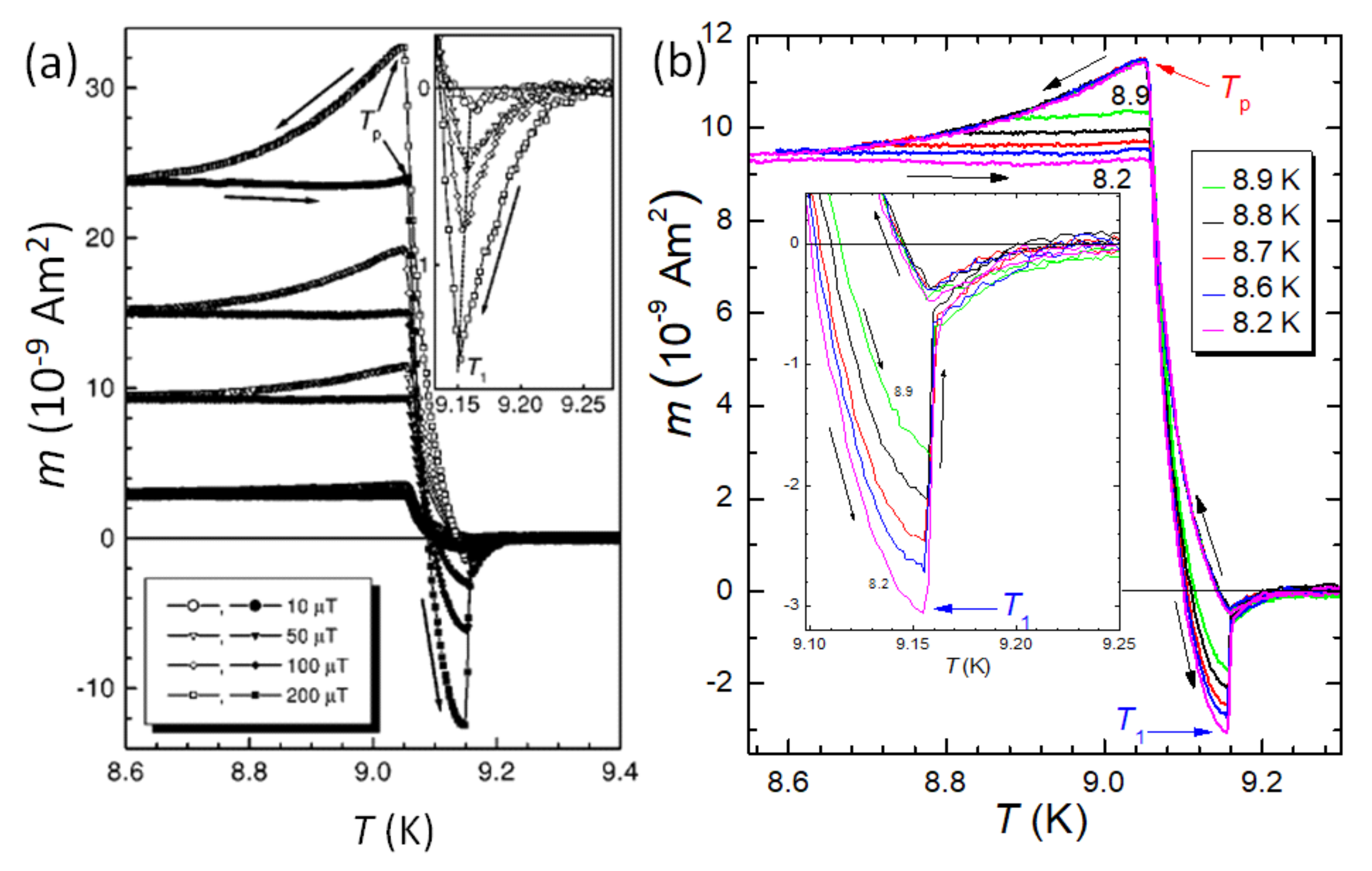
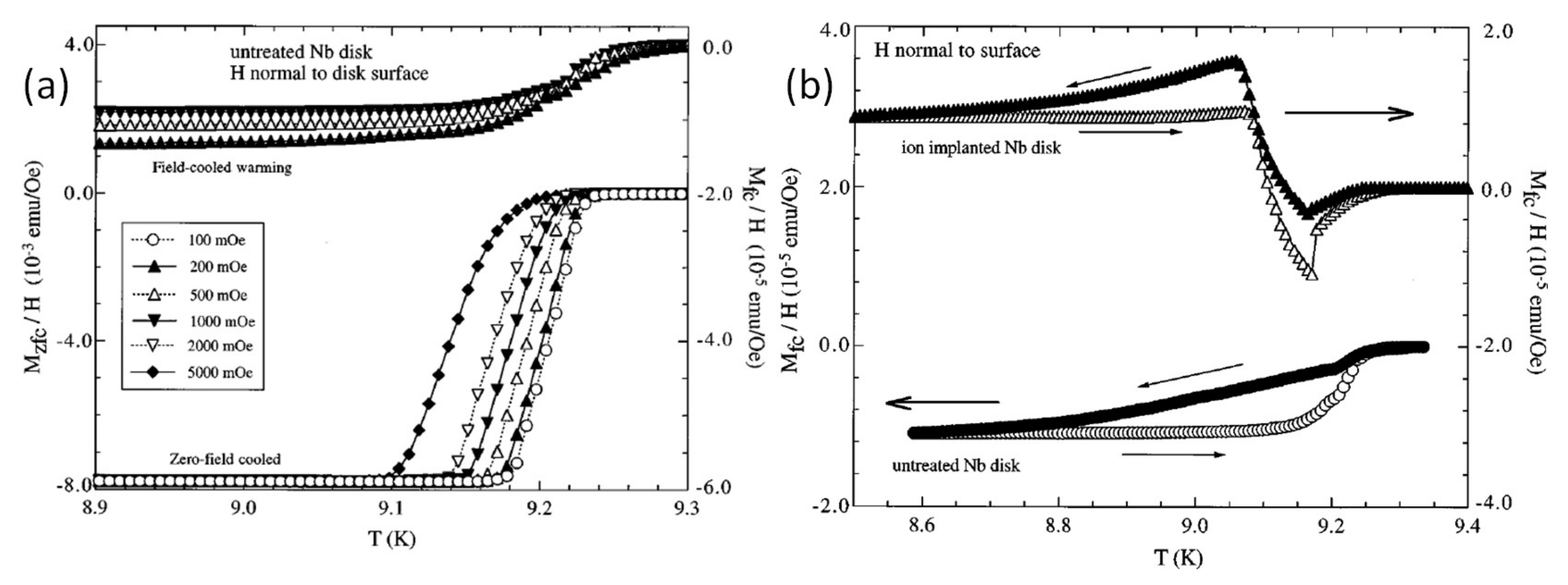
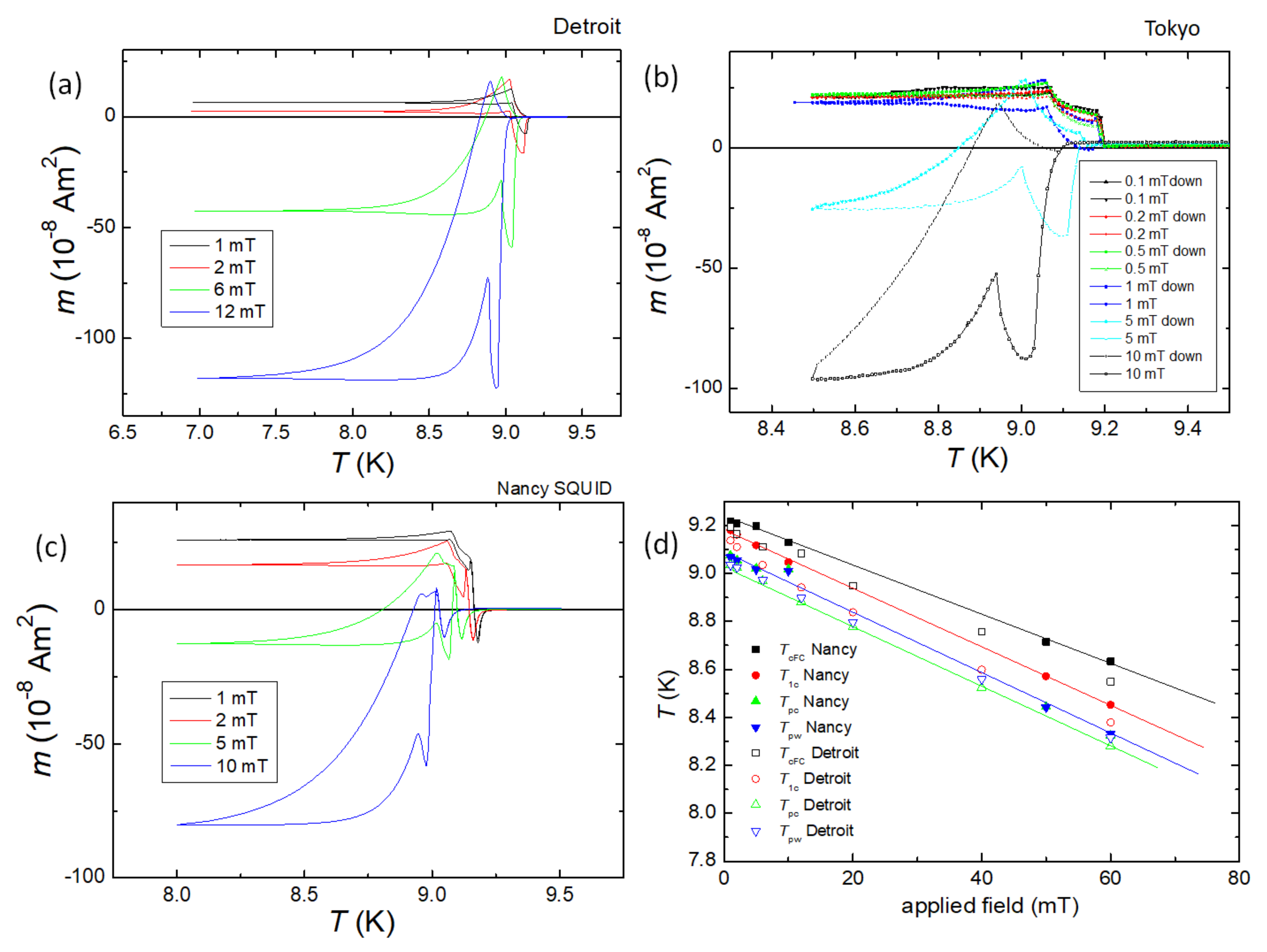
3.2. Observation of PME—Superconducting Transitions

In this Section, we focus on the detailed measurements performed on various Nb disk samples, which were found to exhibit the most clear PME behavior. Niobium (Nb) has a bcc lattice ( a = 0.33 nm and α = β = γ ), is isotropic, and represents a classical s-wave superconductor with a Ginzburg–Landau parameter κ close to the border between type-I and type-II superconductors ( κ ∼0.8–1.0).
The Nb sample studied in Detroit (similar to some other bulk Nb samples seen in the literature) shows a very specific behavior around the superconducting transition region. In previous papers [25,27], this behavior was studied in detail, mainly using the field-cooled cooling (FC-C) and field-cooled warming (FC-W) curves, i.e., the temperature dependence of magnetic moment m ( T ) was measured at constant magnetic field when the temperature is slowly and continuously swept from a temperature where the sample is in a normal state down to a temperature well below the superconducting transition (FC-C) and then the temperature sweep direction is reversed (FC-W). These scans of the magnetic moment, m ( T ) , reveal several characteristic temperatures, namely T 1 ( < T c , onset ) describing the minimum of magnetization, and T p ( < T 1 ), which indicates the maximum of the positive moment [139]. Note here that in some publications, T 1 was also called T u . We must note here that these characteristic temperatures are very important for understanding what is going on in the sample when cooling or warming it in applied magnetic fields.
Figure 5a presents details of m ( T ) transitions measured on a punched Nb disk. The superconducting transitions were measured in small applied magnetic fields (10, 50, 100, 200 μ T) perpendicular to the sample surface generated by the Cu coil (using the low-field option with stationary sample). The temperature was continuously swept at a rate of | d T / d t | = 38 mK/min. The arrows indicate the direction of the measurement (FC-C and FC-W). The temperature T p is defined here as the temperature of the maximum m ( T ) . The inset to (a) shows the definition of the temperature T 1 as the lowest m ( T ) recorded on the diamagnetic side.
Figure 5b presents a similar situation, but here the measurement is performed at a fixed field ( B ext = 0.5 mT) and the temperature was swept at a rate of | d T / d t | = mK/min to reach various minimum values ( T min ) between T 1 and T p and also slightly below T p , which are indicated in the graph. The inset to (b) gives more details close to T 1 . Here, one can see that the m ( T ) curves are nearly reversible in the temperature range between T 1 and T c . Whatever the origin of the paramagnetic moment appearing in the sample between T 1 and T p is, it appears and disappears nearly reversibly when increasing/decreasing the temperature. Furthermore, the onset of the nearly reversible diamagnetic moment can be determined to be at about T = 9.27 K. This moment is fully reversible as long as the temperature did not go close to 9.13 K and below. If the sample was cooled below 9.13 K, one can observe a very slight hysteresis of the m ( T ) curves even in the temperature range above T 1 . The m ( T ) curves below T 1 are fully reversible as long as the temperature T min is not below about 9.07 K during the cooling and warming cycle. For the m ( T ) curves measured at T min < 9.07 K, one can see during warming a sharper decay of the magnetic moment towards its equilibrium value at T = T 1 .
Thus, the field-cooled magnetization results for Nb disks show a paramagnetic moment that has a reversible nature as it appears and disappears at the same temperature T 1 during cooling and warming, respectively. This moment is superimposed on typical diamagnetic superconducting behavior below T 1 and continues to increase in magnitude until the temperature T p . Thus, the appearance of a net positive signal at lower temperatures depends on the relative magnitude of the paramagnetic moment of the sample to that of the diamagnetic moment below the temperature T p .
In Figure 6a–c, FC-C and FC-W m ( T ) -curves are shown in various applied magnetic fields up to 140 mT. A paramagnetic (positive) m ( T ) is observed on FC-C for small applied magnetic fields. This positive moment gradually reduces on the increasing field, and the low-T part of each curve is obtained at negative m ( T ) for all applied fields above 3 mT. However, the FC-W curves all show the characteristic step in the temperature range 8.8–9.2 K.
Figure 7 presents high-field measurements of the PME on a Nb disk (Nb002) which was carried from Detroit to Tokyo. Using the constant temperature sweep rate of a 7T-XL SQUID [145], the measurements were performed with the superconducting coil in the persistent mode. The measurements were performed after the entire magnetometer had been warmed up to room temperature for servicing. In this way, any spurious trapped fields in the coil system can be safely excluded. From this graph we can see that the m ( T ) -curves obtained are always on the negative (i.e., diamagnetic) side, but the fingerprints of the PME can be observed as characteristic steps in the FC-W curves up to 200 mT applied magnetic field.
Figure 8 gives the results of an important experiment which we called ‘shifting the PME’. To estimate the magnitude of the paramagnetic step on the FC-C and FC-W curves measured at B ext = 0.05 mT (see Figure 8a), both the cooling and warming curves below T p were shifted to such a position that the magnetization curves above T 1 and below T p point toward each other. The best results at this value of B ext were obtained for the shift by m shift = 1.33 × 1 0 9 Am 2 . In the detailed view of the transition given in Figure 8b, one can see that the shifted curves combined with the curves above T 1 form a nice, archetypal FC-C and FC-W curve. This is a clear indication that the relative shape of the recorded FC-C and FC-W curves below T p follows an archetypal shape. The crucial change in the superconducting state takes place between temperatures T 1 and T p , where an additional positive moment (superconducting currents) appears in the sample, and this moment stays constant in the sample as long as the temperature stays below T p . It again starts to disappear from the sample when the temperature is raised above T p and it finally disappears completely above T 1 .
Below T c , onset , m ( T ) becomes more negative upon cooling until T 1 is reached (≈9.16 K at the lowest fields), where m ( T ) abruptly turns towards positive values. This increase in m ( T ) continues until another characteristic temperature, T p (≈9.16 K at the lowest fields), is reached, where m ( T ) exhibits a cusplike behavior. Below T p , the relative temperature dependence of m ( T ) appears to correspond to the archetypal FC-C behavior of a superconducting sample not exhibiting the PME. As discussed in ref. [25], another characteristic feature of the PME for the Nb disks is the large hysteresis between the FC-C and FC-W curves with the FCW curves being lower than the FC-C curves. Upon warming, the m ( T ) curves remain practically constant until the moment turns abruptly towards negative values at a temperature essentially the same as T p . Then, at a temperature identical to T 1 , m ( T ) jumps to a less diamagnetic and more probable equilibrium value as the PME appears to vanish suddenly. The similarity in characteristic temperatures where the positive moment first appears during cooling and then disappears during warming as well as where the positive contribution stops increasing in magnitude during cooling and subsequently begins to decrease upon warming suggests that the PME has a reversible nature.
Figure 9 presents the phase diagram of the PME in the bulk Nb disks, constructed from the temperature variation of the characteristic temperatures T 1 , T p , and T c , onset . The inset to Figure 9 presents a schematic phase diagram including surface superconductivity as described by H c 3 ( T ) and the flux flow region described by the irreversibility field H irr ( T ) . The green arrow indicates where FC-C and FC-W measurements are crossing the phase diagram. H irr ( T ) is for most metallic superconductors very close to H c 2 ( T ) [147]. Note also that in the field-cooling experiments with a magnetic field applied, there is always magnetic flux in the sample, and a pure Meissner state will not be reached even if flux is expelled from the sample. The temperature T c , onset , which is slightly larger as the bulk T c , defines the first onset of superconductivity, i.e., the first recording of a diamagnetic moment which occurs at ≈9.23 K for the sample discussed here. All Nb samples from the same Nb sheet we studied in Detroit, Tokyo, and Nancy have T c between 9.23 and 9.27 K. Also given are T c data (magnetically measured to determine H c 2 ) for pure Nb and Nb treated in N 2 from ref. [148]. Any differences determined between the FC-C and FC-W runs for these temperatures are within the size of the data points and are the result of a temperature lag between the sample and the thermometer during the cooling and warming processes. One further can note here that the field dependence for all three temperatures is nearly linear: d T p / d B e = 13.5 K/T (<60 mT) and 11 K/T (>60 mT), d T 1 / d B e = 10 K/T, and d T c , onset / d B e = 8.7 K/T. Our T c , onset -data are higher and d T c = d B e smaller as compared to Weber and Schachinger [148], which may be possible due to different accuracy in measurement/determination of the onset of the diamagnetic signal. However, another explanation is given in ref. [37]: Our T c , onset could directly correspond to H c 3 ( T ) , i.e., the onset of the surface superconductivity. Then, T 1 could correspond to the curve of H c 2 ( T ) and T p to H irr ( T ) , which requires some further analysis using also AC susceptibility measurements (see Section 3.6 below).
In Figure 10a,b the results of applying a magnetic field parallel to the sample surface are shown. Figure 10a, presenting M / H ( T ) and M / H ( T ) , indicates the temperatures T u (which is defined as the first appearance of a paramagnetic moment, and T u T 1 as discussed previously) and T p , where the positive contribution stops increasing in magnitude during cooling [141]. The values of the applied field were, however, not given in [141]. It is also evident from Figure 10a that these temperatures can be identified with certain characteristic features in the ZFC data. T p can be associated with the temperature where the diamagnetic response is at its maximum value and full flux exclusion occurs, while T u represents the temperature where global diamagnetic screening disappears during warming. On the other hand, the FC M / H -data with in-plane field (□) exhibit a more complex but completely diamagnetic behavior, including a hysteresis depending upon whether the sample is being cooled or subsequently warmed through the superconducting transition.
Figure 9. Phase diagram for the PME in bulk Nb disks, constructed using the characteristic temperatures T 1 , T p , and T c , onset . T 1 and T p are taken from both the warming (‘w’) and cooling (‘c’) data. Nb and Nb(N 2 ) represent data from pure Nb and nitrogen-loaded Nb of ref. [148]. The inset shows a schematic phase diagram including surface superconductivity as described by H c 3 ( T ) and the flux flow region described by the irreversibility field H irr ( T ) . The green arrow indicates where FC-C and FC-W measurements are crossing the phase diagram.
Metals 13 01140 g009
Figure 10. PME on Nb disks with perpendicular or parallel magnetic field. (a). M / H recorded in ZFC and FC modes with the magnetic field applied parallel (□) and perpendicular (•) to the Nb disk. The dashed vertical lines indicate the temperatures T u T 1 and T p ; see text. Reprinted with permission from ref. [141]. (b). PME on a Nb disk with the applied magnetic field parallel to the sample surface, measured in the year 2023 in Nancy using a QD PPMS-VSM system [145]. The lines serve as guides for the eye.
Metals 13 01140 g010
Figure 10b presents QD PPMS-VSM [145] measurements performed in Nancy on a rectangular Nb disk stemming from sheet DS4D with the magnetic field applied parallel to the sample surface. Fields in the range between 1 mT and 100 mT were applied. For fields up to 10 mT applied parallel to the sample surface, we observe a positive (paramagnetic) response, which changes into completely diamagnetic signals on further increase in the applied field. Note here also the shift of T c towards lower values when increasing the applied field. This observation clearly shows that PME is also possible in the configuration H sample surface.

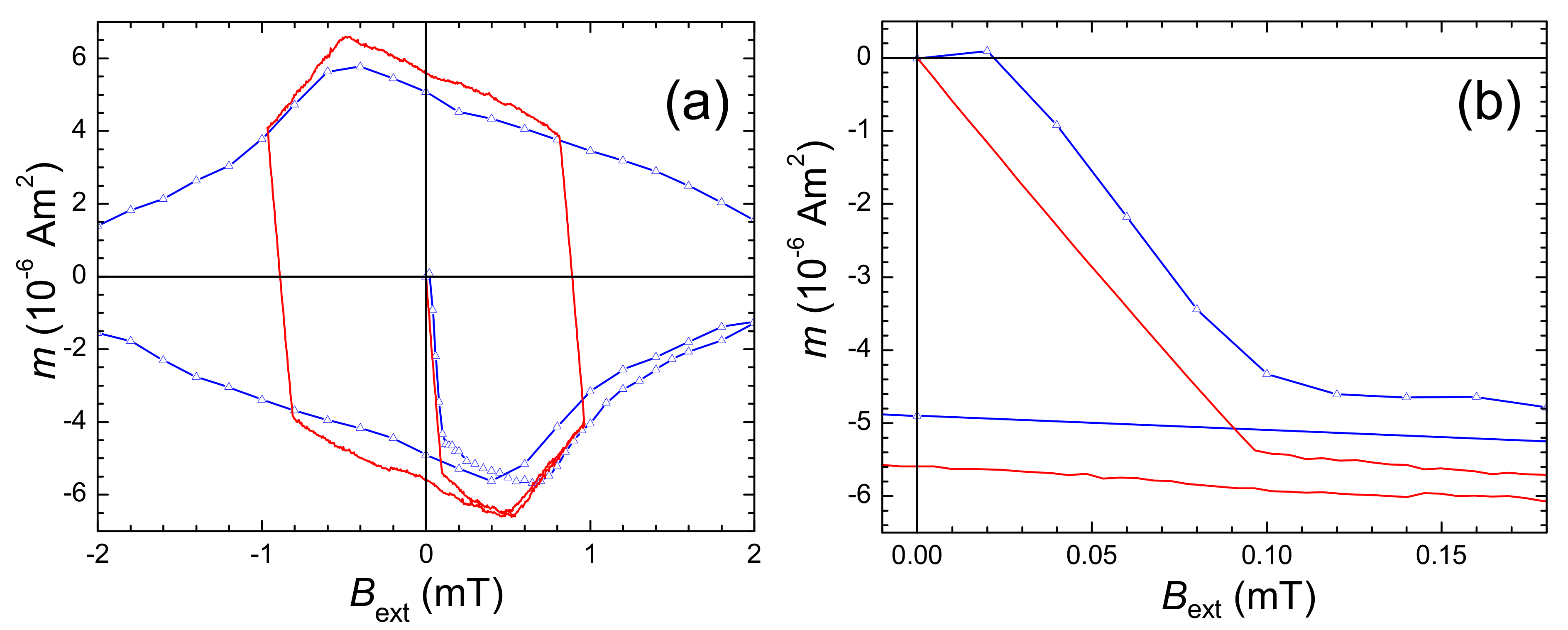
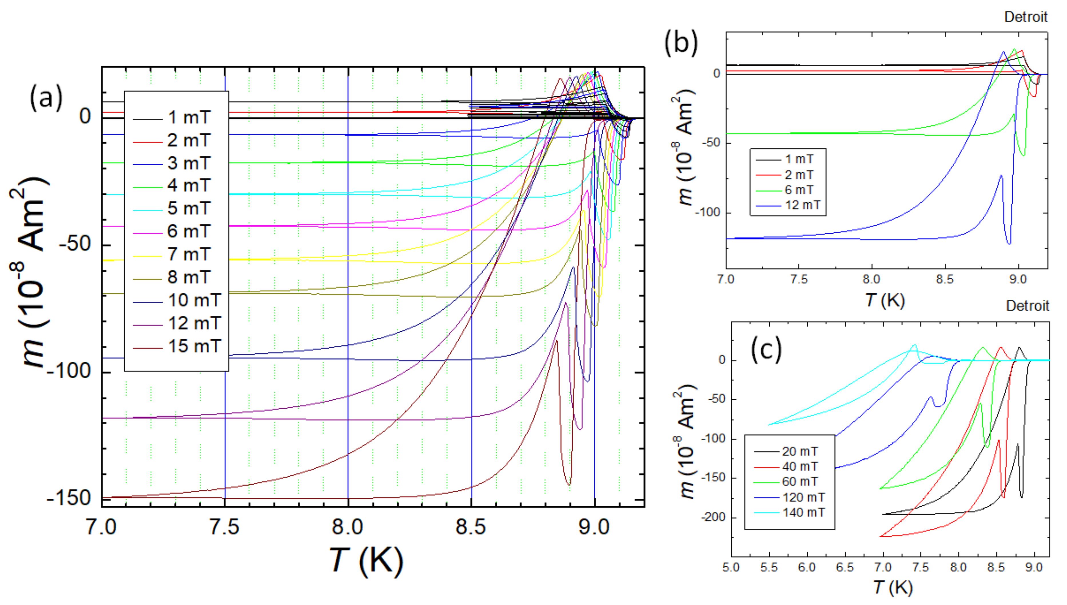
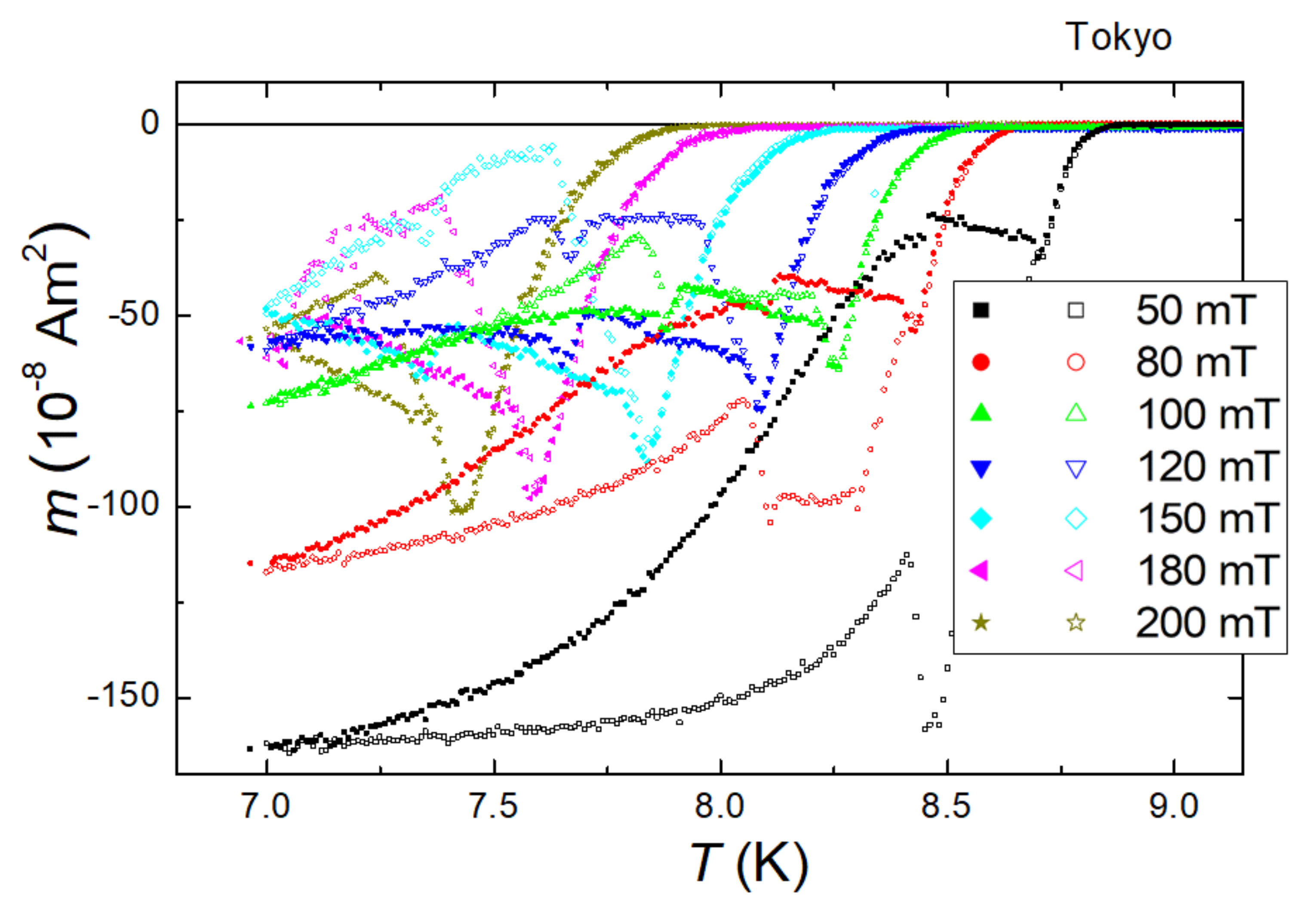
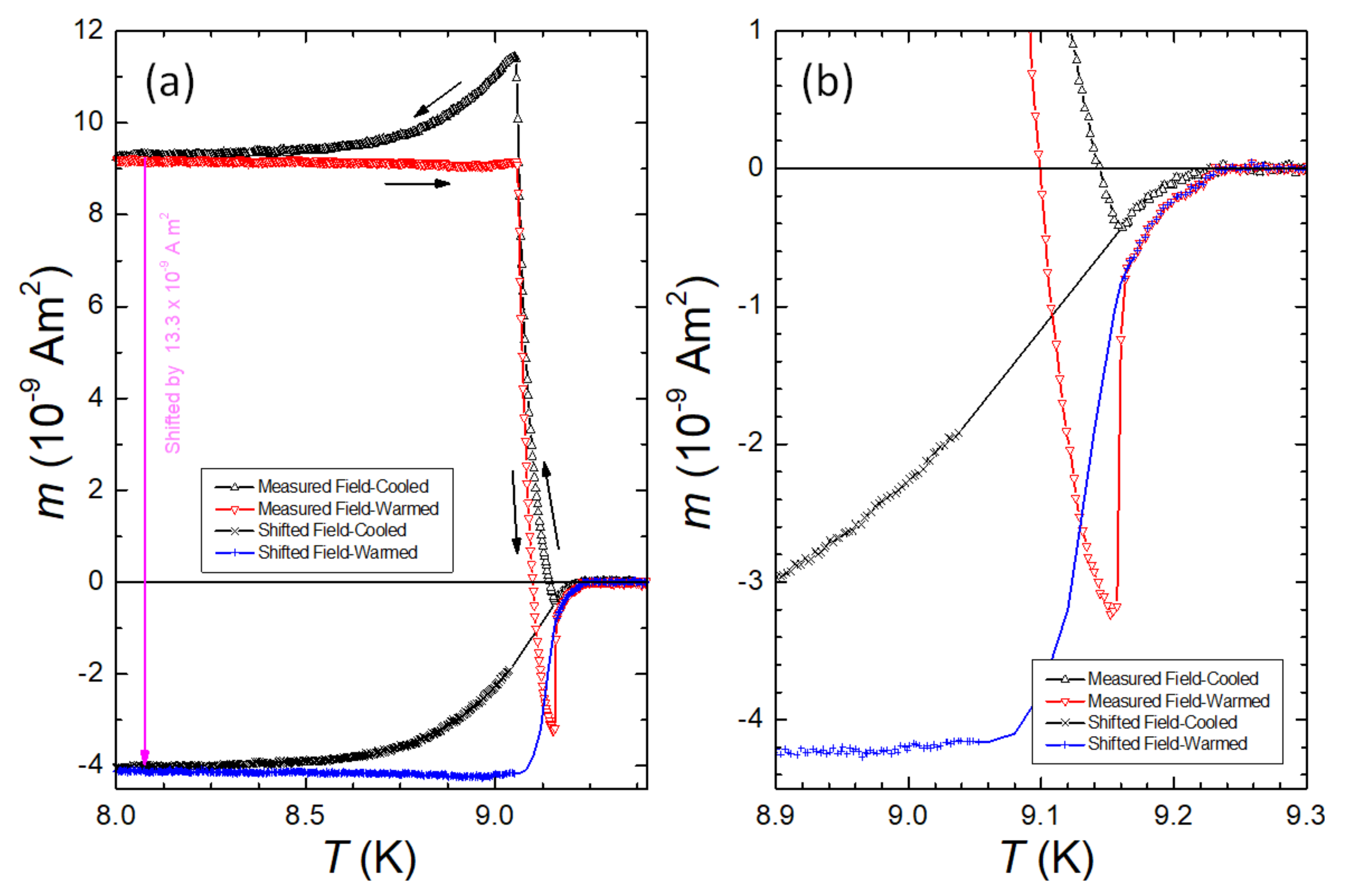
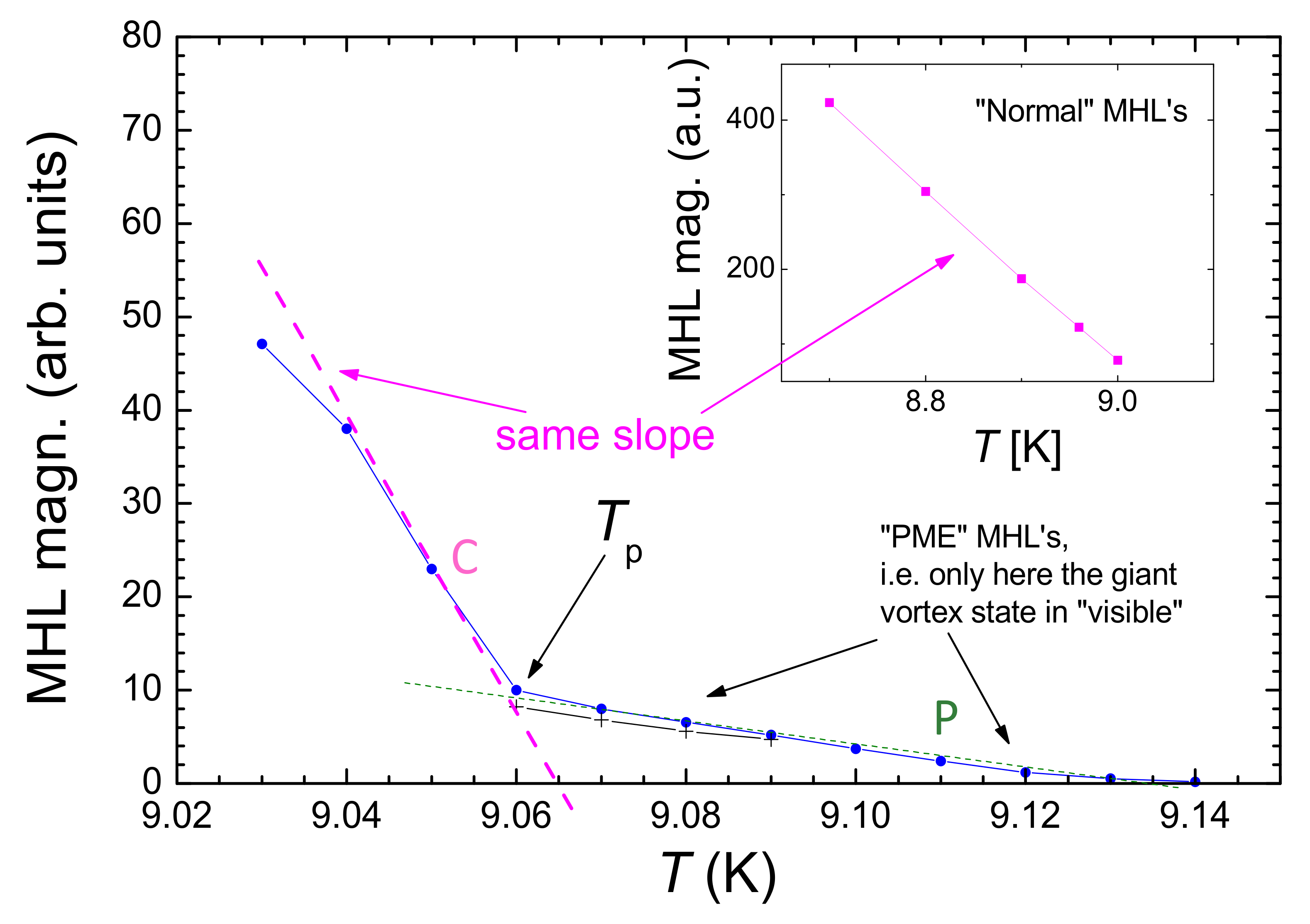
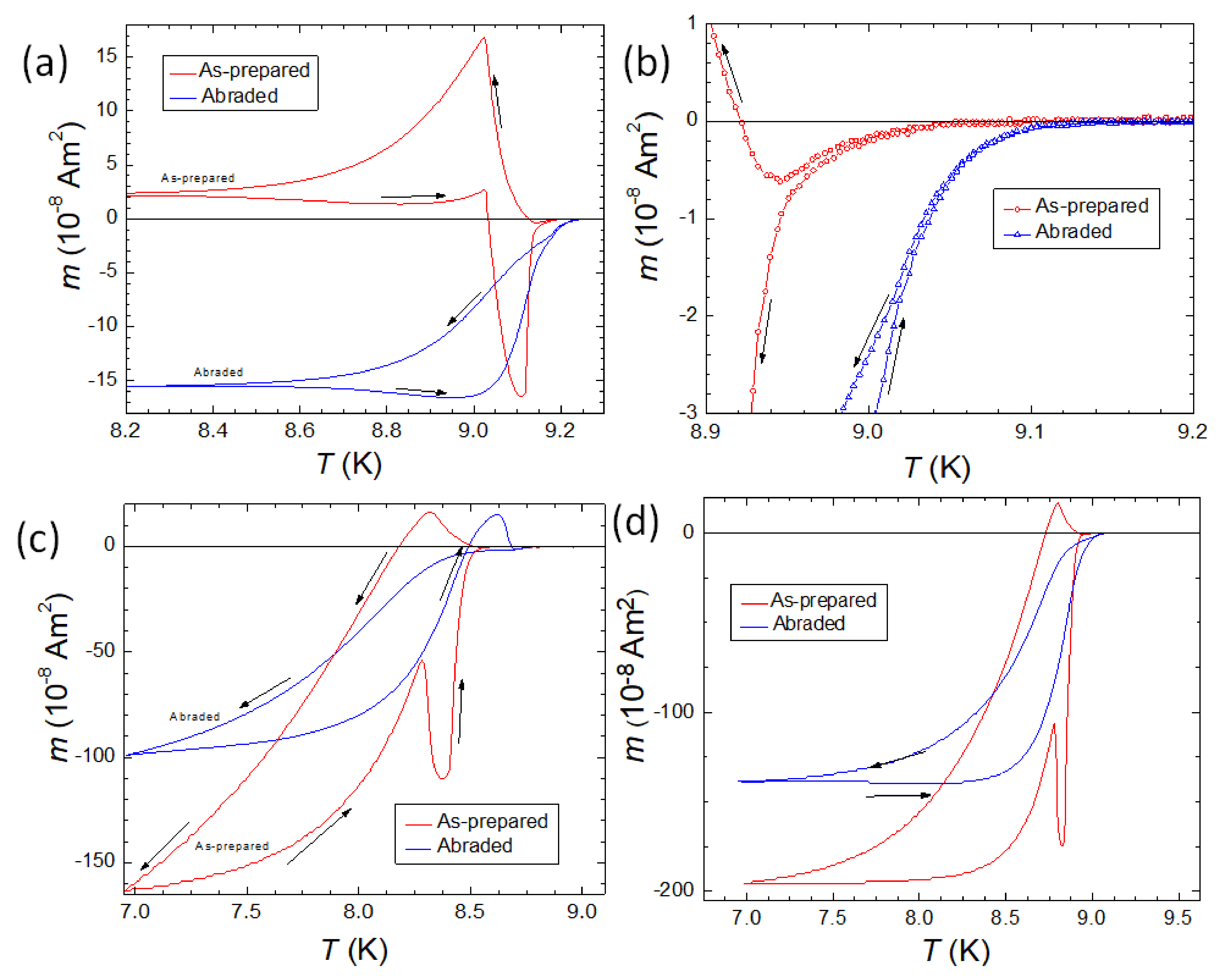
3.3. Magnetization Loops Close to the Superconducting Transition

In order to gain more information about the physical origin of this additional paramagnetic moment, we performed detailed magnetization hysteresis loop (MHL) measurements in three distinct temperature ranges. MHLs of samples exhibiting the PME were rarely investigated in the literature on both Nb and HTSc materials. Kötzler et al. [22] showed some virgin magnetization curves of their Bi-2212 samples, and Thompson et al. [31] have presented an MHL on Nb. The MHL presented in ref. [31] showed a quite specific nearly parallelogram-like shape but there was no detailed analysis nor discussion of this feature. Thus, we take here the opportunity to present a detailed experimental analysis of the MHLs measured on Nb samples exhibiting the PME and a correlation of these results to the widely used PME measurements of magnetic moment at constant magnetic field while the temperature changes.
Figure 11a shows MHLs measured in Detroit on one of the Nb disk samples at temperatures between 8.96 and 9.08 K. These are “archetypal” MHLs of a type II superconductor with the shape given by the field-dependent superconducting currents induced in the sample and vortex pinning in this material. Note here the well-developed central peak located at slightly negative values, but close to zero field as is expected from a bulk, superconducting sample [149,150]. Also shown are the corresponding virgin curves (i.e., the magnetization curves measured when the magnetic field was first applied to the sample after cooling in zero field). The joining of the virgin curve with the main MHL is marked as “A”. All the MHLs presented in Figure 11a were measured in the standard operation mode of the QD MPMS SQUID magnetometer with scan length below 1 cm. In contrast, the MHLs in the transition region between 9.00 K and 9.20 K were measured with temperature steps of 0.01 K using the stationary sample technique. At at field of ∼1 mT, there is still a finite induced magnetic moment and when the direction of the field ramping is reversed, one obtains the so-called “reverse leg” of the MHL given by the process of reversing the induced currents in the sample. This process is qualitatively similar to the process when the virgin curve merges the full MHL.
Figure 11b shows MHLs taken at elevated temperatures in the range 9.05 to 9.10 K, i.e., around the characteristic temperature, T p . While the MHLs measured at 9.00 K and 9.04 K look again more like “archetypal” MHLs, the MHL measured at 9.08 K has apparently a different shape with no clear maximum near to zero field. Even for the MHLs measured at 9.00 K and 9.04 K, one should note that the virgin curves are straight with a very sharp turn when they merge the full MHL (see the area marked as “B” in Figure 11b). All these curves develop a more parallelogram-like shape without any low-field maximum. Note also that the slope of the virgin curve changes between 9.05 K and 9.06 K. There is furthermore a significant change in the shape of the reverse legs of the MHLs. Along with this change, the slope of the reverse leg also changes to being steeper at temperatures below 9.05 K (see also the analysis shown in Figure 13 below).
Below T p , the MHL increases significantly and acquires an archetypal shape of MHL loop of a bulk superconductor with maximum close to B ext 0.
Figure 12a shows MHLs in the very interesting temperature range between 9.07 and 9.14 K, i.e., between T 1 9.16 K and T p 9.05 K. MHLs at these temperatures are found to exhibit several distinct features that probably have the same physical origin as the appearance of the paramagnetic moment during field-cooling in small applied fields. The MHLs have the shape of a nearly regular parallelogram with all turning points being sharp. Note that the reverse legs are entirely linear, all the turning points are quite sharp, and the size of the parallelograms increases with decreasing temperature. Furthermore, the shape of the initial magnetization curve (virgin curve, abbreviated VC) is very linear and then abruptly merges with the nearly field-independent MHL (see Figure 12b). These features cannot be explained by magnetic flux gradually penetrating the superconducting sample, governed by vortex pinning when the field is changed.
Figure 12. Further details on the MHLs measured close to T c . (a) MHLs in the temperature range 9.07 T 9.14 K. (b) The virgin curves (VCs) of the MHLs in the temperature range 9.07 T 9.14 K. The VCs are linear and join the MHLs quite abruptly. (c) The reverse legs of the MHLs 9.05 T 9.12 K. All reverse legs are linear and the ends are quite sharp, i.e., hardly rounded off.
Metals 13 01140 g012
Here it is important to mention again that all MHLs at temperatures close to the transition temperature were determined from the SQUID voltage change generated by the stationary sample. This method is very “safe” as it eliminates spurious signals that may be generated when the sample is moving during the measurement. However, this method cannot be used at higher fields and consequently at lower temperatures where the induced moments are large and we cannot measure anything but reversible screening currents. Fortunately, at lower temperatures we can use the conventional measurement of the magnetic moments in the point-by-point method with the sample moving (the scan length should be as short as possible) over a distance in a magnetic field generated by the build-in superconducting magnet. At lower temperatures, the induced magnetic moment is quite large and so, the possible spurious signals due to moment motion are relatively small.
Figure 12b shows more details of the virgin curves of the MHLs measured after cooling down in zero field. The slope S = d m / d H ext of virgin curves recorded at T = 9.06 K and above is remarkably lower (by about 20%) as compared to the slope of all virgin curves recorded at T = 9.05 K and below. The major change of the virgin curve slope takes place just below T p where a remarkable change in the shape of the MHLs also takes place. Additionally, the slope S of the initial curves changes below T p with the magnitude and temperature dependence of this change corresponding to the step observed in the zero field-cooled susceptibility curves [25]. At the temperature T p the VC shape also changes. Below T p , the VC bends when approaching the MHL, indicating gradual penetration of magnetic flux into the sample.
Finally, Figure 12c illustrates the field reversal on the MHLs at temperatures from 9.05 to 9.12 K. In this temperature range, one can see very straight reversal legs with very sharp and regular turning points at the MHL at field reversal. This behavior is again a very important characteristic feature of the bulk Nb disks, closely related to the presence of the PME.
Figure 13 shows the temperature dependence of the magnitude of MHL (i.e., the maximum induced magnetic moment, m max ( T ) ). m max ( T ) is nearly linear below the temperature T p going sharply towards zero at about 9.065 K, as indicated by a dashed line (🞍 🞍 🞍 🞍 🞍). The inset to Figure 13 presents the same analysis for the temperature range 8.7 T 9.0 K, i.e., the range where the “normal” MHL shape is found. The slope obtained here and the slope of the magenta dashed line in the main panel are the same. However, above 9.06 K, m max ( T ) abruptly changes the slope and decreases, again nearly linearly, but with a slope being about one order of magnitude smaller, as indicated by the dashed green line (🞍 🞍 🞍 🞍 🞍). Thus, in the temperature range T p T c , the PME-MHLs are visible, giving an indication of the giant vortex state.
It is obvious from this graph that the m max ( T ) dependence can be formally separated into two components, one (we will call this component “C”) that goes sharply to zero at T = 9.06 K T p , and another component (we will call this component “P”) that has a much weaker temperature dependence. The component P is not “visible” at temperatures below T p , where the P component is overwhelmed by the larger C component and the magnetic moment is given primarily by the dominant component C, which describes the classic situation of flux pinning of Abrikosov vortices. The situation changes below the characteristic temperature, T p , where the magnetic moment from the component C is (practically) zero and the m max ( T ) -dependence is entirely given by the component P that diminishes only at temperatures close to T 1 or higher.
Figure 13. Evaluated details of the hysteresis measurements. The graph gives the MHL magnitude (maximum induced magnetic moment) as a function of temperature. The blue datapoints () give the data obtained from the MHLs; the black crosses (+) represent the data from a second run. The slope from the archtypal MHLs as shown in the inset () and the slope of the component C in the main panel (🞍 🞍 🞍 🞍 🞍 ) are the same. It is obvious from this graph that at T p an abrupt change in the MHL shape takes place, and the normal flux pinning vanishes. At T > 9.06 K, the component P is measured follwing a completely different slope (🞍 🞍 🞍 🞍 🞍).
Metals 13 01140 g013
Considering both the shape and character of MHLs at various temperatures, and also the FC and ZFC curves studied in detail in refs. [25,139,140], we can attribute the component C to the conventional behavior of a type-II superconductor, where induced currents are governed primarily by vortex pinning. The origin of the component P is still not fully understood. This component is obvious only above T p , where the C component diminishes to zero, but the character of the m max ( T ) -dependence indicates that the P component is present in the sample also at temperatures below T p . We thus believe that the component P of the induced magnetic moment is responsible for specific superconducting behavior of Niobium below the transition temperature including (but not limited to) the appearance of that positive magnetic moment when the sample is cooled in small applied magnetic fields (i.e., the Paramagnetic Meissner effect).

3.4. Manipulating the PME

To investigate the influence of the sample surfaces on the PME, several experiments were performed in Detroit: (i) the surfaces of the Nb disks were abraded (thereby the sample thickness was reduced by about 10%), and (ii) the sample edges were treated using sandpaper. Sanding off the edges of the sample did not lead to a change in the PME characteristics, so these data are not shown here. In contrast, abrading the sample surface (sample Nb2) was found to have a significant effect on the PME of the Nb disks as illustrated in Figure 14a–d. DC magnetic fields of 2 mT (a,b), 20 mT (c), and 60 T (d) were applied. The as-prepared sample (red datapoints, sample Nb1) exhibits all the features of the PME as discussed before, whereas the abraded sample does not show any signature of the PME at any applied field. Note also when defining T c , onset as the temperature of the onset of a diamagnetic moment on the cooling curve (FC-C) and disappearance of the moment on the warming curve (FC-W), the abraded sample Nb2 exhibits a T c , onset , which is about 0.05 K higher than that of the Nb disk with PME (sample Nb1).
Thompson et al. [32] demonstrated that ion implantation into the sample surface area can create the PME in a sample which did not show the PME prior to irradiation. Since these Nb superconducting samples exhibiting the PME have a surface microstructure containing defects, which are known to increase the critical current density, it is reasonable to expect that introducing defects through ion implantation, e.g., might enhance or even create the PME in other Nb disks. For the Kr-ion bombardment, disks of 6.4 mm diameter were punched from an untreated, cold-rolled, 0.25 mm thick sheet of niobium (99.8% purity, Johnson-Matthey) as well as from a 6.45 cm 2 (1 in 2 ) section of the same sheet that had both sides ion implanted with 200 keV Kr ions at a dose of 6 × 10 16 /cm 2 . During the following magnetic measurements in the SQUID system in Detroit, the samples were kept stationary. The result of this procedure is presented in Figure 15a,b. From these figures, it is very clear that the PME can be induced in Nb disks by implanting Kr ions to a depth of about 120 nm below the surfaces of the disks. Enhancing the T c variation and the effective pinning strength from existing surface defects which result from the ion bombardment are important factors in the development of the PME. By creating a surface defect structure with greater relative depth into the thicker Nb disks, these lower- T c regions serve as more effective pinning sites which produce inhomogeneous field variations whose temperature dependences could result in the PME’s characteristic behavior. In order to further our understanding of the effect that the ion implanting has upon the magnetization characteristics, one should note that the Kr ions penetrate uniformly to a depth of 40 nm below the surface and then the concentration drops off to a negligible value beyond 120 nm. Thus the observed magnetic behavior is strongly affected by just the first 120 nm below the two surfaces of the disks. Clearly the ion bombardment has created an inhomogeneous superconducting sample with a T c variation as evidenced by the appearance of a second diamagnetic transition at 9.07 K. It is known, e.g., that the T c of Nb is easily reduced by oxidation and strains. Furthermore, Halbritter [151] has shown that an enhanced oxidation is promoted around defects and serrations on the Nb surfaces so that the defect regions can extend down to several microns below the surface. Consequently, it is plausible that the Kr ions have the greatest impact on these regions by reducing the T c and extending their depth below the surface. Secondly, the ion implanting has produced sites with extremely strong flux pinning as indicated by the narrowing of the ZFC M / H transition width of the largest diamagnetic change. The inducing of PME through ion implantation on a sample which previously did not exhibit PME signatures helps further the understanding of PME.

3.5. Time Evolution of PME in Nb

In Figure 16a, we show the evolution of the superconducting transitions measured on the same sample (round disk punched from the original Nb sheet, sample Nb002) in the timeframe from 1997 to 2023. The first measurements on this disk were carried out in Detroit using the stationary sample technique in 1997 (see Figure 16a). The sample was then carried to Tokyo (SRL/ISTEC, Div. 3) and the measurements were repeated in the summer of 1999 using a 5T-SQUID with ultra-low field option (Figure 16b). Finally, the sample was carried to Europe and remeasured at IJL Nancy using a QD SQUID MPMS3 with VSM and AC options (Figure 16c). In Figure 16d, a comparison of the characteristic temperatures T 1 , T p , and T c FC (i.e., T c obtained from FC data) is shown. It is remarkable to see that the surface structure of this Nb disk is so stable that all the major elements of the PME transitions are repeated, even though the sample was carried only in a simple plastic box together with some silica gel [152].

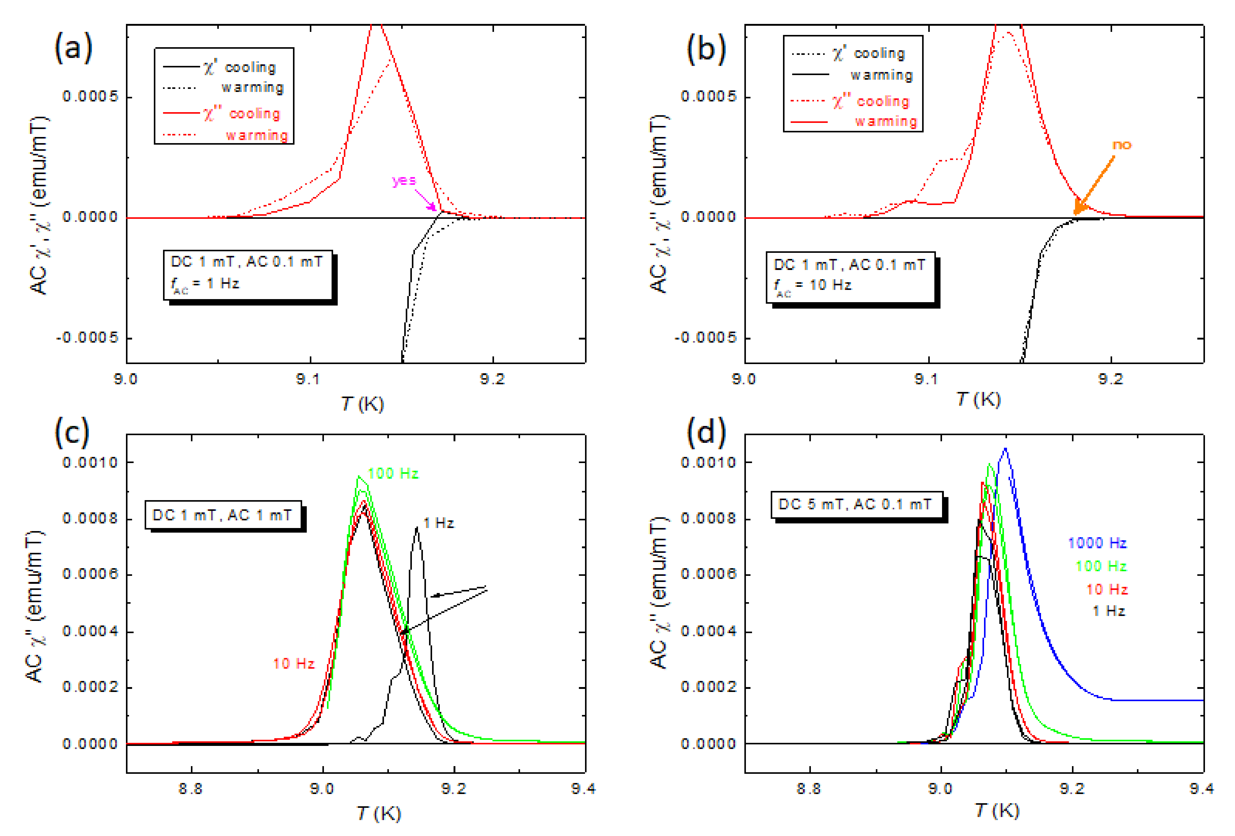
3.6. Ac Susceptibility Measurements on Nb Disks
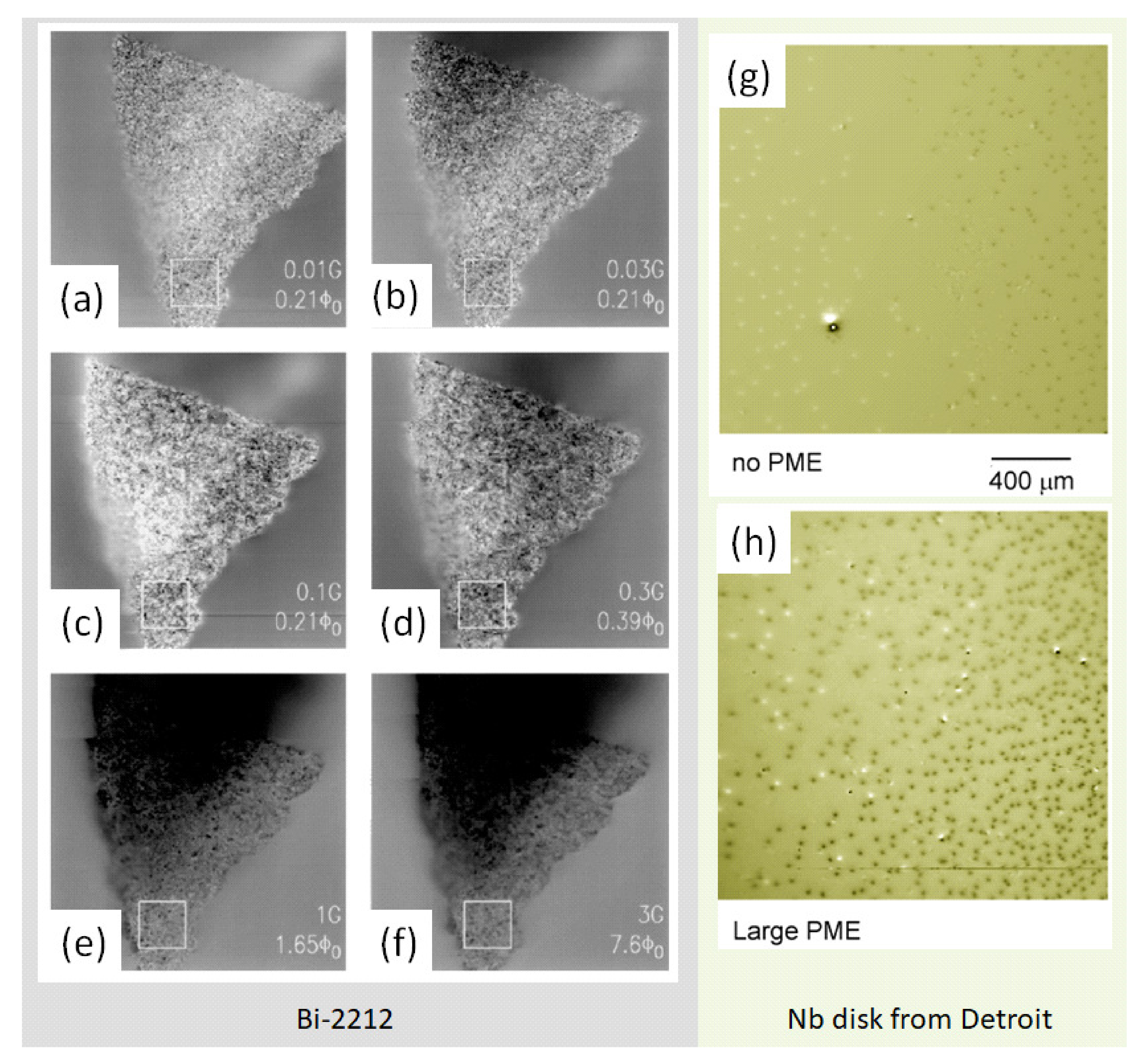
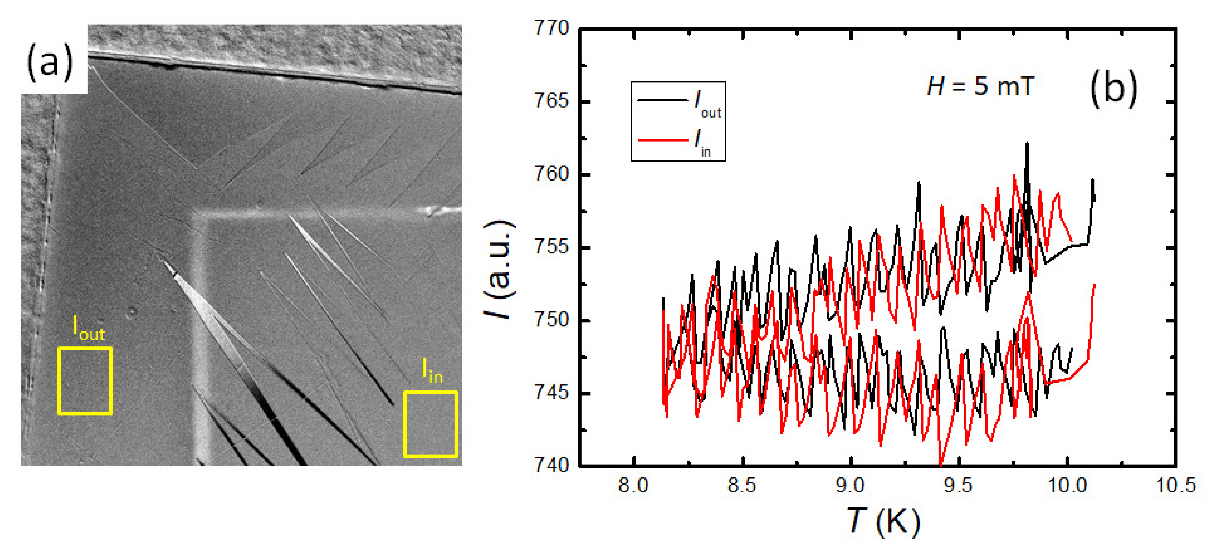
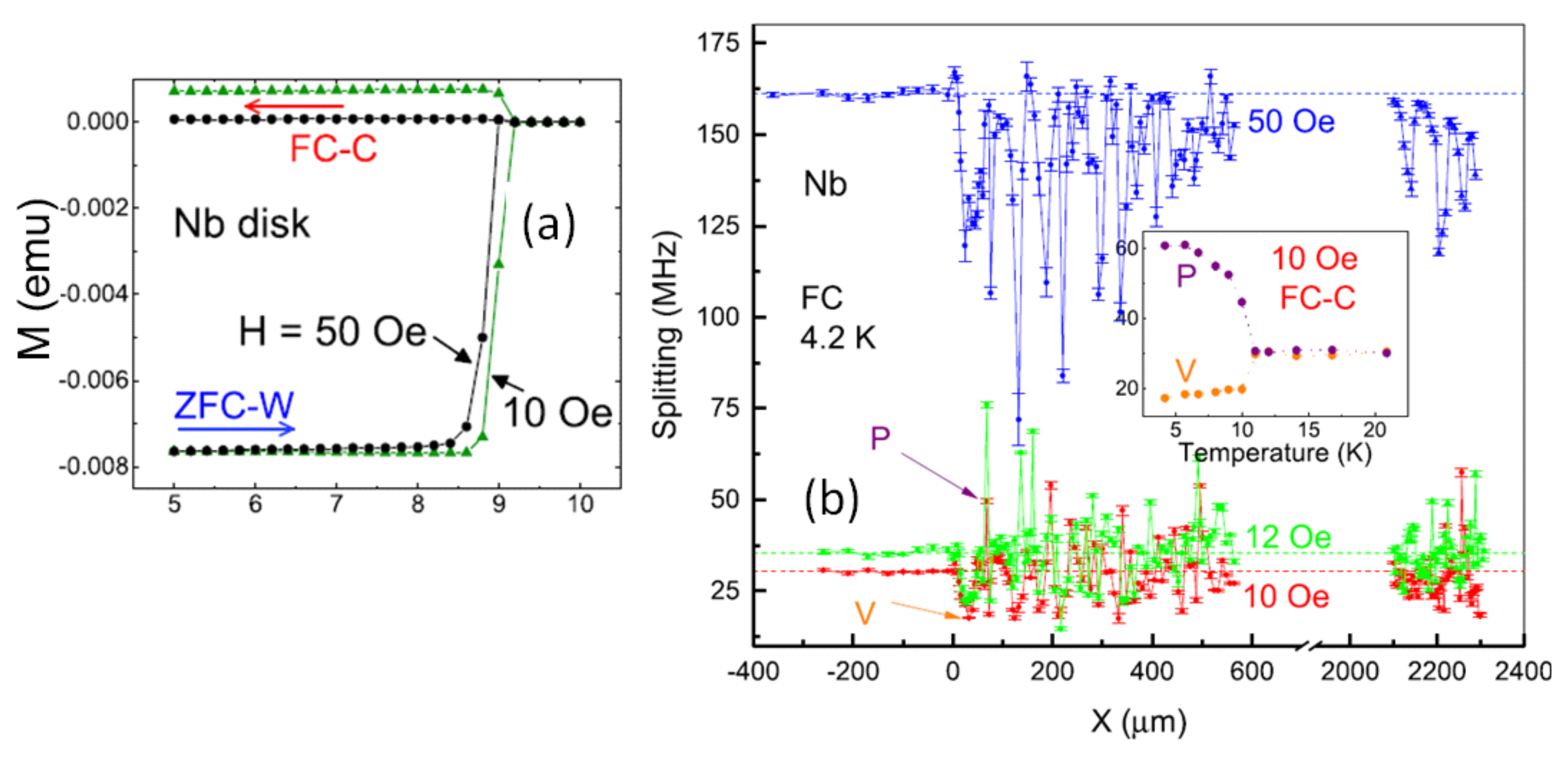
The PME was observed using AC susceptibility on HTSc Bi-2212 [16,24], and much later by Ge et al. [37] on ZrB 12 crystals. The signatures, which indicate the presence of PME, are completely different for the HTSc and the conventional superconductors, as for the HTSc PME is revealed by a strong frequency dependence on the left (low-T) side of the loss peak in χ (measured frequencies, f = 17 mHz up to 1.7 kHz) as well as a dependence on the AC field amplitudes ( h ac = 0.4–12 μ T), showing a linear response [24]. To analyze the data for the influence of flux creep effects, the higher harmonics were analyzed in [16]. In the case of ZrB 12 [37], an anomalous positive peak is seen in the χ -data ( f = 333 Hz, h ac = 0.1 mT), and no frequency dependence of the loss peak in χ was reported. The positive peak in χ was termed diffraction paramagnetic effect (DPE), and enabled the determination of T c surface as well as the onset of diamagnetic response, T irr (see also Figure 23 below).
Measurements of the AC susceptibility were performed in Nancy using the AC-option of the MPMS3 SQUID system [145] to obtain further information on the details of the superconducting transition of the Nb disks from Detroit (see Figure 17a–d). These experiments were carried out after ensuring the PME effect in the Nb disks by DC SQUID measurements. Figure 17a gives details of the recorded superconducting transition ( χ , χ ) recorded in a DC field of 1 mT, an AC amplitude of 0.1 mT, and a frequency of 1 Hz. The full lines ( and ) indicate data recording during cooling (sample cooled down to 8.6 K), and the corresponding dashed lines (🞍 🞍 🞍 and 🞍 🞍 🞍) give the data for warming. A tiny positive signal is obtained for χ recorded during cooling, similar to the case of ZrB 12 . Increasing the AC frequency to 10 Hz makes the positive peak vanish, as shown in Figure 17b.
In Figure 17c, the frequency dependence of χ at a DC field of 1 mT and an AC amplitude of 1 mT is shown. All data were recorded during cooling and warming. There are only small differences seen at the high-T side of the loss peak, and the peak height increases upon an increase in the frequency. However, at 1 Hz there is a strong difference between cooling and warming modes. On cooling, the same path as for the higher frequencies is followed ( T peak ∼9.05 K), but on warming, the peak is shifted to about 9.17 K and a characteristic shoulder at the low-T side appears. We must note here that the measurement during cooling was carried out with a sweep rate of 72 mK/min, whereas the warming was measured with a rate of 30 mK/min, so this may have an influence on this observation. On the other hand, this was done in all the measurements and the entire measurement run was repeated three times, but only the data recorded with an AC amplitude of 1 mT and at a frequency of 1 Hz showed this behavior. The higher position of the loss peak recorded during warming falls directly in the region between the two characteristic temperatures T p and T 1 , so this loss peak may have directly to do with the formation of a giant vortex state. We also must note here that there is also a hysteresis in the c h i -data (not shown here). This requires further investigation. Figure 17d gives the frequency dependence of the AC loss peak taken at a DC field of 5 mT and an AC amplitude of 0.1 mT. The data taken at 1000 Hz obviously suffer from a skin effect at the metallic surface. No trace from PME (positive moment) is visible in all the curves. Thus, we may summarize these AC experiments by saying that traces of PME in Nb disks can only be observed at low frequencies (1 Hz) and small applied DC fields (1 mT) and AC amplitudes (1 mT). These observations demonstrate the presence of PME signatures also in the AC susceptibility measurements, and the signatures are present in both the real and imaginary part of the susceptibility.

4. Magnetic Imaging

Several different imaging techniques were already applied to superconductors exhibiting PME; among them are magneto-optic imaging [8,153,154], the scanning SQUID technique [155,156], the imaging using color centers in diamond [157,158], and low-energy muon spin spectroscopy (LE- μ SR) [108].
We will start the discussion with the scanning SQUID experiments performed by Kirtley et al. [112] on HTSc Bi-2212 samples. Figure 18a–f present the spatial distribution of magnetic flux in and around the HTSc sample. The grey contrast scale is chosen so that white corresponds to the largest and black to the smallest (often negative) flux value. In all cases the flux is plotted relative to the flux introduced by the external field, which sets the grey level outside the sample. One overall feature, which is observable by the human eye, is the difference between the paramagnetic magnetization (i.e., the sample is brighter than the background) at weak applied magnetic fields, and a diamagnetic signal (i.e., the sample is darker than the background), in the pickup loop at strong applied magnetic fields. For weak external magnetic fields the inhomogeneity of the magnetic flux is clearly visible and gives rise to a broad distribution of the local fluxes as the sample is a polycrystalline bulk. Here, it must be noted that all images were taken at T = 4.2 K (allowing the performance of the SQUID loop in the same condition as the sample). The sample was cooled through T c with the external magnetic field applied, and the field was still on when reaching 4.2 K. Thus, in this form of the scanning SQUID technique, measurements in the very interesting region around T c cannot be performed. Nevertheless, the images obtained nicely reproduce the situation shown in Figure 1b, where the fields smaller than 30 μ T (0.3 G) produce a positive m ( T ) , and fields of 100 μ T (1 G) and 300 μ T (3 G) yield a diamagnetic signal. The authors of [112] claim that the images provide direct evidence for spontaneous orbital currents, but it is not possible to determine the origin of such orbital currents from the images. An attempt to repeat the same scanning SQUID experiment on the Nb disks from Detroit is represented in Figure 18g,h. Figure 18g gives the result obtained at T = 4.2 K when field-cooling the sample (abraded Nb disk without PME) in a field of ∼0.16 μ T (1.6 mG). The image shows many vortices (white and black colors denote vortices of opposite direction), which are quite well-separated from each other (annihilation effects). In contrast, the same image of a Nb disk with PME (h) taken at ∼0.28 μ T (2.8 mG) reveals a much larger number of vortices being present within the image frame, and also the number of black vortices is much higher than the number of white vortices. Furthermore, there is a field gradient from left to right, but the two types of vortices are not so well separated as in (g). Hence, the scanning SQUID technique can produce very interesting images of the vortex distribution, but the temperature limitation to 4.2 K does not allow an observation of the giant vortex state around T p , i.e., close to T c .
The flux compression effects and the giant vortex state would be interesting objects to be directly observed by magnetic imaging methods. However, there are two main problems: the required high field sensitivity and the low temperatures of the superconducting transition of Pb and Nb. For magneto-optic imaging [8,153,154], the spatial sensitivity depends on the distance of the indicator layer to the sample surface, and as the sample surface cannot be treated by polishing, the resulting distance is quite large, thus leading to reduced spatial resolution. This also affects the field sensitvity, which must be quite high to resolve single flux quanta. The temperature problem, which is often seen in magneto-optic cryostat systems operating with a helium gas stream, is nowadays nicely overcome by optical cryostats being cryocooled, which enable even lower temperatures to be reached while the sample is illuminated [159]. After ensuring the presence of the PME on the Nb disks in Nancy, we also performed magneto-optic imaging in Liège (group of Prof. Silhanek, [160]). Figure 19a,b present the MO imaging results on a Nb square cut from the original Nb sheet. The applied magnetc field is 5 mT, which was kept on during the temperature sweep from 10 K to about 8 K. Figure 19a gives the MO image, where the outer edge indicates the edges of the MO indicator film, and the inner L-shape indicates the edges of the Nb sample. Figure 19b gives the recorded flux in the two yellow boxes (I out , I in ) as shown in (a). It is obvious that the flux profiles do not reveal an intensity difference between the area inside and outside of the sample, which would indicate trapped flux in the sample. This implies that the available field sensitivity is not high enough to reveal a signature of a giant vortex state. Thus, further new experiments on Nb samples are required to finally ”see” a trace of the giant vortex state. In contrast, Vlasko-Vlasov et al. [161] have imaged a paramagnetic state when field-cooling a RbEuFe 4 As 4 sample below the magnetic transition point. The measurements resemble the PME; however, in contrast to the PME close to T c , the magnetic transition is here far below T c and the applied magnetic fields are much higher (20 mT and more) as well.
Another interesting experiment was carried out by Nusran et al. [162] (Figure 20) employing the non-invasive magnetic field sensing using optically detected magnetic resonance of nitrogen-vacancy centers in diamond, short NV magnetometry. The experimental apparatus incorporates a confocal microscope optimized for NV fluorescence detection. The fluorescence is stimulated by the green off-resonant 532 nm laser excitation and low-energy levels are populated by the microwave radiation applied using a single silver wire loop antenna coupled to an MW frequency generator. A thin diamond plate with an ensemble of NV centers embedded near the surface (∼20 nm depth) is used as the magneto-optical sensor. The spatial resolution of the sensor is determined by the effective size of the probe, which is essentially a convolution of the focal volume with the NV distribution in the diamond plate. This leads to a disk-like probing volume of thickness ≈20 nm and diameter ≈500 nm. A detailed review of the NV-centers and NV magnetometry can be found in refs. [157,158].
Figure 20a presents m ( T ) measured on a Nb disk-shaped crystal using a Quantum Design MPMS SQUID system. Shown are the ZFC-W and FC-C curves measured for fields of 1 and 5 mT (10 and 50 Oe). Both curves reveal the PME, but no details of the superconducting transition as seen in Figure 5. Figure 20b presents recorded FC profiles of the magnetic induction for applied magnetic fields of 1.0, 1.2, and 5 mT (10, 12, and 50 Oe). Measurement was performed at T = 4.2 K. The signatures of the paramagnetic Meissner effect (PME) are observed in various random regions for low magnetic fields. Cooling in 1 mT (10 Oe, red datapoints) and 1.2 mT (12 Oe, green datapoints) applied magnetic fields results in very similar profiles. The inset to (b) presents a temperature-resolved measurement in a 1 mT (10 Oe) magnetic field upon FC-C. The peak (P’) and valley positions (‘V’) of the inset are indicated by arrows in the main panel.
To investigate the Meissner effect in a superconductor/magnet system, the depth profile of the local magnetic susceptibility of a Au (27.5 nm)/Ho (4.5 nm)/Nb (150 nm) trilayer was measured by low-energy muon spin spectroscopy (LE- μ SR) [108]. The main idea of this experiment was to demonstrate an intrinsic paramagnetic Meissner effect, which was prediced for s-wave superconductors with broken time reversal symmetry as a result of an emergent, unconventional odd-frequency superconducting state, competing with conventional (i.e., even-frequency) superconductivity [102]. The antiferromagnetic rare-earth metal Ho breaks time-reversal symmetry of the pair correlations in Au and has a thickness that is comparable to the known coherence length for singlet pairs in Ho to ensure pair transmission into Au. The Au layer is necessary since a Meissner state cannot be probed by muons directly in a magnetic material due to their rapid depolarization in a strong magnetic field. (LE- μ SR) offers extreme sensitivity to magnetic fluctuations and spontaneous fields of less than 10 μ T (0.1 G) with a depth-resolved sensitivity of a few nanometers [163,164]. To probe the depth dependence of the Meissner response in Au/Ho/Nb by LE- μ SR, an external magnetic field ( B ext ) is applied parallel to the sample plane and perpendicular to the muon initial spin polarization (oriented in the x-z plane). To investigate the paramagnetic Meissner effect, implantation energies in the 3–6 keV range were used to determine the B loc ( z ) profile in the Au layer. The overall recorded T c of the trilayer film is 8.52 K.
Figure 21a–d present the results from such an experiment performed at 5 K (a,b) and at 3 K (c,d). The data recorded at 10 K (i.e., above T c ) are shown by and the magenta line corresponds well to the applied field of 101 G. The measurement at 3 K shows the most significant PME response within the Au layer. A conventional Meissner effect (i.e., B loc ( z ) < B loc ( z ) ( 10 K ) ) is measured in Nb up to the interface with Ho, where the contribution of spin-singlet Cooper pairs to the screening supercurrent J x ( z ) is larger than that due to the long-ranged spin-triplet pairs. The PME is obtained in the Au layer (i.e., B loc ( z ) > B loc ( z ) ( 10 K ) ), indicating a paramagnetic screening where B loc ( z ) appears nonmonotonic with depth (see the blue curves in Figure 21a,c).
The advantage of this technique is the high spatial resolution inside the trilayer structure, but requires the antiferromagnetic Ho layer to break time-reversal symmetry of the pair correlations in Au. The data clearly reveal the intrinsic PME within the Au layer, generated via the superconductor proximity effect. Thus, an intrinsic PME was observed in an s-wave superconducting sample, which is thus not related to the field-trapping/compression mechanism. As an outlook to future experiments, the authors of [108] state at the end of their paper that future experiments should explore ways to harness the magnetization generated by odd-frequency superconductivity in order to explore the potential for driving magnetization-reversal processes in the superconducting state [165].

5. Discussion

After the presentation of the various PME results obtained on a large variety of metallic superconductors, it is necessary to discuss the various models applied to explain the PME in these samples. The first model, the flux trapping/compression and the Giant Vortex state, explains the PME as an extrinsic feature, depending on the sample surface or local distribution of superconducting properties. This is in contrast to the other explanations ( π -junctions, odd-wave superconductivity) being intrinsic, i.e., a material property.

5.1. Flux Compression and Giant Vortex State

The most important model being applied to the PME of metallic superconductors is the flux trapping/compression [82] and the giant vortex state [85,86]. As shown by Koshelev [82], a kind of inhomogeneous cooling of a superconducting sample, i.e., when field-cooling a sample, vortices may be expulsed from the sample along the edges, and other flux is then trapped in the sample center. Continuous cooling then leads to a broadening of the flux-free regions and compresses the flux in the center even further by the vortex Nernst effect, as described by Huebener [5]. The same picture would apply if the sample surfaces have a higher T c than the remaining bulk of the sample. Such situations may be realized by specific sample surfaces, e.g., due to oxidation effects [151].
Based on a numerical, self-consistent solution of the Ginzburg–Landau equations for a fixed orbital quantum number L, Moshchalkov et al. [85,86] proposed that the PME arises from the flux compression with integral number of quantum flux L Φ 0 , where Φ 0 denotes the flux quantum, trapped in the sample interior. This model refines the approach of Koshelev and adds the surface superconductivity, described by the third upper critical field, H c 3 ( T ) , into the model. When field-cooling a sample, one crosses the phase diagram (see, e.g., Figure 9 and 23 below) on a horizontal line at H 0 . Thus, we come first through an area of surface superconductivity as H c 3 ( T ) > H c 2 ( T ) , before entering the region with Abrikosov vortices below H c 2 ( T ) . These vortices may form a liquid as the flux pinning sets in only below H irr ( T ) , the irreversibility field. This region may be small for the metallic superconductors, but it does exist especially at low T. For lower temperatures, the Shubnikov phase prevails as commonly described in the textbooks.
By studying the PME in mesoscopic superconducting Al and Nb disks, Geim et al. [62] gave a clear indication that the quantized flux trapped at the third critical field, H c 3 , is responsible for the PME, which further supports the theoretical predictions of refs. [85,86]. Thus, the flux compression mechanism seems to be more universal to explain the PME observed in both HTSc (here, the superconducting grains of polycrystalline sampes also form mesoscopic objects) and conventional superconductors (LTSc).
To explain the ideas in more detail, we assume now that inside a superconductor there are no pinning centers with the size comparable to the giant vortex core. In this case, a giant vortex state is stabilized only by the sample surface and this state is reversible as long as the orbital quantum number L is kept constant. However, as the temperature goes down, the multiquanta vortex state may decay rather quickly into Abrikosov vortices with ϕ 0 , once the conservation of L is violated. As soon as the Abrikosov vortex lattice is formed at T < T sat , flux pinning centers, which are relatively small in comparison to the giant core, can be very efficient to pin the ϕ 0 vortices, thus leading to the onset of irreversibility. The irreversibility should then be considered as the consequence of the onset of the variation of L, initiating the crossover between the giant vortex state ( L = const.) and the Abrikosov vortex state ( L = 1), which should occur around the H c 2 ( T ) line. Expressed differently, in superconducting samples, where the surface pinning plays the dominant role in stabilizing the giant vortex state, the irreversibility line H irr ( T ) seems to lie, in fact, quite close to the upper critical field H c 2 ( T ) .
By cooling down a superconductor in a fixed applied field (field-cooling mode), the H c 3 ( T ) boundary in the phase diagram (see Figure 9 and Figure 23) is crossed at a particular point, which corresponds to a certain orbital quantum number, L. Note here that the H c 3 ( T ) -line is not a homogeneous line, but cusplike according to L [85]. In the calculations performed in refs. [85,86], it was assumed that the orbital quantum number L, found according to the location of the crossing point between H c 3 ( T ) and H = const., is kept constant also below the H c 3 ( T ) line. The conservation of the orbital quantum number L in the superconducting state can result from pinning of the giant vortex state, corresponding to a ringlike superconducting order parameter nucleated at the sample boundary at H c 3 ( T ) . In this case, the sample boundary is the source for pinning the giant vortex state. The conserved value L = const. is determined by the applied magnetic field. If sufficiently small fields are applied, a state with L = 1 (i.e., Φ = Φ 0 ) can be realized. It also must be mentioned here that for L = 5, the vortex core and the area, where additional field b ( r ) is generated due to the flux compression, are considerably larger than for L = 1.
As the temperature further decreases, the order parameter grows and pushes the magnetic field into the core. It can be clearly seen from the calculations of refs. [85,86] that for the trapped L > 1 vortex, the field b ( r ) is localized in the area where the superconducting order parameter is strongly reduced. This reflects a very general flux expulsion property of a superconductor which causes either normal diamagnetic Meissner effect with complete flux expulsion for the state L = 0 without a core or flux compression (i.e., PME) in the vortex core for L > 1 . Topologically, L = 0 and L < 0 states are qualitatively different, since for the latter, flux is expelled both inwards and outwards. When the former dominates, PME can appear.
Figure 22a plots the magnetic flux captured inside or expelled out of a Hall magnetometer of 2.5 μ m width at 0.4 K, due to the presence of superconducting disks ( Δ Φ = B H = 4 π M , ref. [166]). The two disks were fabricated simultaneously by thermal evaporation and differ only in their diameters. The strongly oscillating behavior clearly seen for the larger sample is due to size quantization. Each jump corresponds to a change in the number of vortices inside the disk, which can either form an array of single quantum vortices or assemble into a single giant vortex. The latter configuration is generally expected at applied magnetic fields between the second and third critical fields, H c 2 < H < H c 3 , that is, it corresponds to the surface superconductivity in a confined geometry. The smaller sample (□) does not exhibit the rapidly oscillating field dependence, and its Meissner response remains negative over the entire field interval. Such qualitatively different behavior can be related to the fact that, in the smaller sample, the superconductivity is suppressed by only ∼3 flux quanta, ϕ 0 , entering the disk area, while ∼20 ϕ 0 are necessary to destroy superconductivity of the larger disk.
The observations of Figure 22a,b may seem to be in contrast to the various studies of the PME on macroscopic samples, where the PME was normally found in very low fields and gradually disappeared with increasing field. However, one should take into account that even the lowest fields in these experiments allowed many thousands of flux quanta inside the sample interior, which is in stark contrast to the mesoscopic samples. One can observe that, with decreasing thickness of the mesoscopic disks, the sign reversal of the Meissner effect tends to occur at lower fields and the magnitude of the PME becomes larger. In contrast, no qualitative difference in behavior is observed between disks of circular and square shapes.
The origin of the PME became evident [62] when comparing the field dependence of the Meissner effect discussed above with the magnetization response measured by sweeping the magnetic field at a constant temperature (abbreviated C-T regime). Instead of a single magnetization curve characteristic of macroscopic superconductors, the spatial confinement of a mesoscopic sample gives rise to an entire family of magnetization curves, which correspond to different vortex states. Several superconducting states can be realized at the same applied magnetic field (up to five such states, as can be seen in Figure 22b), but only the state with the most negative C-T magnetization is the thermodynamically stable one [167,168]. All other states are metastable and become observable due to the presence of the surface barrier of the Bean–Livingston type [169]. The recent theory is in good agreement with similar C-T curves, as reported previously.
Figure 22b demonstrates that the paramagnetic states reached via field-cooling are all metastable. Indeed, the FC data predictably fall on the C-T curves because only these distributions of the order parameter are allowed by quantization. However, among all possible states at a given magnetic field, the system unexpectedly ‘chooses’ the metastable state with the most positive possible magnetization. Only if we remove the proper screening in the experimental setup can a metastable high-magnetization state eventually relax to the corresponding stable state on the lowest curve. The same result was obtained when the experiment was carried out in a more controllable manner by applying an oscillating magnetic field at a constant field, H. One can verify that, according to Figure 22b, an oscillating (fluctuating) field moves the system down the ladder of curves towards the equilibrium state. The following consideration may answer the question of how, when cooling down, the system can end up in the most thermodynamically unfavorable state. Superconducting states in a confined geometry can be characterized by a quantum number L, which corresponds to the number of nodes in the distribution of the complex order parameter Ψ along the sample circumference. For the case of a giant vortex and an array of single-quantum vortices, L has a simpler meaning. L then represents the angular momentum and the number of vortex cores, respectively. Transitions between the various states with different L are of first order and lead to (little) jumps in the magnetization data.
Close to the third critical field (i.e., the critical field of surface superconductivity), H c 3 , the magnetic field is distributed homogeneously and it requires the ‘high-temperature’ magnetic flux Φ HT Φ 0 ( L + L 1 / 2 ) [170] to initiate a giant vortex state with the momentum L inside a superconducting disk of radius r. As the temperature decreases below the surface superconducting transition, the superconducting sheath at the disk perimeter rapidly expands inside, compressing the giant vortex into a small volume (see the inset to Figure 22b; here, the case l r is considered). The compressed flux inside a giant vortex is equal to Φ 0 L , that is, Φ HT is practically conserved for L 1 . When, at H c 2 , the giant vortex splits up into L single-quantum vortices, the captured flux changes little. At this point, it must be taken into account that the magnetic field also penetrates at the disk boundary, giving rise to an additional flux through the disk of the order of π r λ H B , where H B is the field strength in the λ -layer at the surface. The magnetization response of the sample is paramagnetic as long as the low-temperature value of the total flux, Φ LT < Φ 0 L + π r λ H B , is larger than Φ HT . For a superconducting cylinder, H B = H and the PME appears at relatively large L > ( r / λ ) 2 and its amplitude is rather small ( μ λ / r ). The plate geometry significantly enhances the PME because the field H B is increased by demagnetization effects [82]. In case the central region of the sample is occupied by a vortex or vortices as small as the disk area, one can approximate H B H ( r / t ) , where t denotes the sample thickness. This results in a paramagnetic response μ λ / t , which is considerable even for macroscopic thin disks. This result for μ can be directly compared with the result of Figure 8a, where m shift = 1.33 × 10 9 Am 2 (disk with t = 0.127 mm) was obtained for the additional paramagnetic moment appearing. Furthermore, the plate geometry also leads to an earlier start of PME [62].
From these observations, it can be concluded that this persistence of L down to low temperatures is responsible for the PME. Thus, especially the various observations of the PME made on the Nb disks (i.e., the measurements of m ( T ) and the special shape of the magnetic hysteresis loops, m ( H ) ) can be effectively explained using the giant vortex model and flux compression.
Another interesting experiment in the literature considered the vortex state in the presence of the PME, which is still unclear. In the literature, it is reported that not all samples show PME, even with similar nominal composition. Furthermore, it was demonstrated that the PME disappears after abrading/polishing the surface of the sample or even can be created by irradiation, indicating that surface configurations, such as defects and pinning centers, do play an important role for the PME. Recently, a broad region of non-monotonic vortex interactions was discussed for multi-band and type-II/1 superconductors [171,172,173,174]. A giant PME may appear due to such non-monotonic vortex interactions, which may facilitate the trapping of magnetic flux [174]. As experimental evidence of PME in type-II/1 superconductors was lacking in the literature, Ge et al. [37] have studied the PME in a ZrB 12 single crystal. In this work, the authors have introduced the concept of fast and slow cooling of the samples, i.e., (i) fast (slow)-field cool-warming (F(S)FC-W): the sample was cooled with a large (small) cooling rate of 5 K min 1 (0.03 K min 1 ) to the required temperature under a magnetic field of H, then the magnetization was measured with increasing temperature; (ii) slow-field cool-cooling (SFC-C): the magnetization was measured with decreasing temperature at a rate of 0.03 K min 1 to the desired temperature under various magnetic fields; see also Figure 2e.
The fast cooling enabled the PME to be observed only when cooling down the sample at a sufficiently high cooling rate (5 K min 1 ). At the small cooling rate of 0.03 K min 1 , the extra flux trapped through surface superconductivity has enough time to escape from the sample interior due to flux diffusion, resulting in a stable and more ordered vortex state at low temperatures. This is another important aspect for many other observations of the PME, which must be considered in the planning of the experiments.
From their data obtained on the ZrB 12 crystal, the authors have constructed a phase diagram, where they have interpreted the T c , onset as T c surface , and T irr as the onset of a diamagnetic response in the measurement of χ . The resulting phase diagram (Figure 23) shows all characteristic fields/temperatures for a sample exhibiting PME, and can directly be compared to Figure 9, showing the results of the bulk Nb disk. Thus, it is obvious that Nb and ZrB 12 share the same origin of the PME, but the vortex interactions of both materials are different.
Figure 23. (a) Temperature dependence of the magnetization in the FFCW mode at 0.5 mT (5 Oe). (b) Phase diagram for the PME in FFCW mode. The third critical field H c 3 is defined from the onset of DPE in the in-phase ac susceptibility measurements; H c 2 is defined from the intersection of two linear fits of the M ( T ) curves above and below the onset; T i r r is derived as the onset of a diamagnetic signal on the in-phase ac susceptibility curve. The solid and dashed lines are plots of the empirical formula H ( T ) = H 0 [ 1 ( T / T c ) 2 ] n . The black crosses (‘×’) show the field locations where magnetic relaxation curves are measured (not shown here, Figure 6 of [37]). Image reproduced with permission from ref. [37].
Metals 13 01140 g023
All these observations of PME in Nb, ZrB 12 , and the mesoscopic Al samples directly imply that the PME is not an ‘uncommon’ or ‘exotic’ feature, but fits fully into the picture of a superconducting material when the contribution of surface superconductivity as described by H c 3 ( T ) > H c 2 ( T ) is of significance. Furthermore, effects of demagnetization may play an important role for the observation of PME. It must be noted here that the flux trapping/compression effects may also apply to granular HTSc materials, where micrometer- or nanometer-sized grains exist together with an intergranular medium. This was also pointed out by Geim et al. [62].

5.2. π -Junctions and d-Wave Superconductivity

This explanation of PME was only valid for granular HTSc materials such as Bi-2212, until Govindaraj et al. [107] came up with PME in boron-doped diamond film. If intergranular π -junctions are present, spontaneous equilibrium supercurrents could emerge. Closed loops containing the odd number of π -junctions will lead to spontaneous equilibrium supercurrents. It is important to mention here that the observation of a paramagnetic m ( T ) signal is not sufficient to decide about the physical origin of the PME. This was also the main conclusion of the previous review by Li [97]. Thus, more dedicated experiments are required, such as microwave absorption or the measurements of flux noise by Magnusson et al. [114]. Here, the noise spectral density is related to the out-of-phase component of the AC susceptibility according to the fluctuation–dissipation theorem. The suppression of the magnetic-flux noise with the application of a weak magnetic field strongly favors a description in terms of large localized magnetic moments, which become polarized by the superimposed field. The estimated magnitude of the magnetic moments is in accordance with the expectations of a model based on π -loops, where each loop can be associated with a magnetic flux approximately equal to Φ 0 / 2 . On the other hand, an explanation of the PME based on flux trapping/compression cannot be ruled out even for the HTSc Bi-2212 polycrystalline samples, as the surfaces of the small, superconducting grains may have different superconducting properties and thus may enable flux trapping/compression effects.
In a recent contribution, Govindaraj et al. [107] studied electrical transport and magnetic properties of two different BDD thin films (electron density 1.4 resp. 2.6 × 10 21 cm 3 ) and found two magnetic effects at low magnetic fields (millitesla range), coexisting with superconductivity: (1) the Wohlleben effect or paramagnetic Meissner effect (PME) and (2) pressure-induced spin glass, such as an anomaly in low-field susceptibility. Here, we must note that the m ( T ) -data recorded in this case are not really similar to the Bi-2212 data shown in Figure 1b (second panel), as there is no diamagnetic signal close to T c , and all m ( T ) -curves recorded turn towards a diamagnetic signal for all applied fields when further cooling down the sample. The differences between the HTSc and Nb as discussed by Kirtley et al. [112] (Section 2.1) were also not observed. The resistance data on the same samples, also shown in [107], are found to increase prior to reaching T c for all fields up to 5 T. Govindaraj et al. thus claim that both effects (1) and (2) observed in their work imply the emergence of π -junctions, which may be a plausible assumption for this type of material.
So, one can conclude here that the explanation of PME by spontaneus currents in π -junctions is still alive, but more experimental data are still necessary.

5.3. Odd s-Wave Superconductivity

The odd s-wave superconductivity is only obtained in the combination of an s-wave superconducting material with a nonsuperconductor (e.g., Ag, Cu, Au) or with a ferromagnetic material. Cooper pairs may enter into the normal metal or the ferromagnet in a thin layer according to the proximity effect. The samples involved here are thin-film multilayers, and so the direct measurements of m ( T ) or m ( H ) do not reveal the details of the underlying physics. So, a specially designed magnetic imaging technique using low-energy muon spin spectroscopy (LE- μ SR) on Nb-Ho-Au trilayers was designed and carried out in [108]. In this experiment, the paramagnetic contribution was revealed within the Au-layer (superconductivity induced by the proximity effect; see Figure 21), which represents a direct proof that odd s-wave superconductivity provides a paramagnetic contribution.
Very recently, van Weerdenburg [175] showed that in ultrathin Al films (8.5 ML film) a paramagnetic contribution from odd s-wave superconductivity gives rise to an enhanced magnetic penetration depth and an enhanced vortex size due to the Meservey–Tedrow–Fulde (MTF) effect [176]. The vortex size was measured in this paper via d I / d U -maps in STM/STS, and no magnetization data were reported. However, this is the first experimental proof that odd s-wave superconductivity may also play a role for pure, superconducting materials when reaching the atomic limits.
It is obvious that odd s-wave superconductivity does not provide an explanation for the PME in the bulk or mesoscopic s-wave superconductors, but provides an unique way to design superconductor/ferromagnet structures for superconducting spintronics [165], which may have important consequences for such applications.

6. Conclusions and Outlook

To conclude, we have presented a review on the experimental data of PME observed on various metallic samples using either magnetometry, AC susceptibility, or various magnetic imaging techniques. Several different materials were found in the literature to exhibit the PME, and several different shapes of samples were involved; single crystals, polycrystalline bulks, nanowires and nanowire arrays, thin films, mesoscopic samples patterned from thin films, multilayers, and bulk wires (in the case of MgB 2 ) were studied. Among them, the bulk Nb disks, the Al and Nb mesoscopic films, and the ZrB 12 crystals were analyzed in detail to refine the flux compression and giant vortex state models. Thus, there are now well-defined theoretical explanations for most features of PME. However, not all features of the PME are fully understood. Hence, there is still room for more detailed measurements to further elucidate those partially understood features. With the development of new imaging techniques such as photoresponse imaging [177], new insights into the origin of PME may become possible.
The more recently discussed odd s-wave superconductivity in multilayer samples may bring up a paramagnetic Meissner effect, which offers an unique way to design superconductor/ferromagnet structures for superconducting spintronics.
Future work on PME will consider very thin films of metallic superconductors, where significant progress has been made to fabricate uniform atomic monolayer films of Pb, Nb, Al, V, and MgB 2 [175,178,179,180,181,182]. Giant PME may appear from non-monotonic vortex interactions as predicted in [174]. In addition, the fabrication of new superconducting polymorphs by nanostructuring [183] may open new ways to induce PME, and superconducting spintronics may develop new application possibilities. These all present interesting possibilities for PME in future work!

Author Contributions

Conceptualization, L.P. and M.R.K.; formal Analysis, L.P., C.-S.C., T.H., A.K.-V. and M.R.K.; investigation, L.P., C.-S.C., T.H., A.K.-V. and M.R.K.; supervision, T.H. and M.R.K.; Writing—Original Draft Preparation, L.P., A.K.-V. and M.R.K.; Writing—Review and Editing, all authors. All authors have read and agreed to the published version of the manuscript.

Funding

This research received no external funding.

Data Availability Statement

Datasets obtained and analyzed during the study are available from the corresponding author on reasonable request.

Acknowledgments

We would like to thank A. Silhanek (U Liège, Belgium), R. Prozorov (Ames Lab., USA), L. E. Wenger (†), and M. Murakami (ISTEC/SRL, Div. 3/Shibaura Institute of Technology, Tokyo, Japan) for valuable contributions and/or discussions on the PME in Nb and other metallic superconductors.

Conflicts of Interest

The authors declare no conflict of interest.

References

  1. Meissner, W.; Ochsenfeld, R. Ein neuer Effekt bei Eintritt der Supraleitfähigkeit. Naturwissenschaften 1933, 21, 787–788. [Google Scholar] [CrossRef]
  2. Tinkham, M. Introduction to Superconductivity, 2nd ed.; Dover Publications Inc.: New York, NY, USA, 1996. [Google Scholar]
  3. Savitskii, E.M.; Baron, V.V.; Efimov, Y.V.; Bychkova, M.I.; Myzenkova, L.F. Superconducting Materials, 1st ed.; Plenum Press: New York, NY, USA; London, UK, 1973. [Google Scholar]
  4. Rose-Innes, A.C.; Rhoderick, E.H. Introduction to Superconductivity, 2nd ed.; Pergamon Press plc.: Oxford, UK, 1978. [Google Scholar]
  5. Huebener, R.P. Magnetic Flux Structures in Superconductors, 2nd ed.; Springer: Heidelberg, Germany, 2001. [Google Scholar]
  6. Poole, C.P. (Ed.) Handbook of Superconductivity, 1st ed.; Elsever: Amsterdam, The Netherlands, 1995. [Google Scholar]
  7. Buckel, W.; Kleiner, R. Supraleitung. Grundlagen und Anwendungen, 7th ed.; Wiley-VCH: Weinheim, Germany, 2013. [Google Scholar] [CrossRef] [Green Version]
  8. Koblischka, M.R. Magnetic Properties of High-Temperature Superconductors; Alpha Science International Ltd.: Oxford, UK, 2009. [Google Scholar]
  9. Pitaevskii, L. Phenomenology and Microscopic Theory: Theoretical Foundations. In Superconductivity. Conventional and Unconventional Superconductors; Bennemann, K.H., Ketterson, J.B., Eds.; Springer: Berlin/Heidelberg, Germany, 2008; Volume 1. [Google Scholar]
  10. Mangin, P.; Kahn, R. Superconductivity. An Introduction; Springer: Cham, Switzerland, 2017. [Google Scholar]
  11. Svedlindh, P.; Niskanen, K.; Norling, P.; Nordblad, P.; Lundgren, L.; Lönnberg, B.; Lundström, T. Anti-Meissner Effect in the BiSrCaCuO System. Phys. C 1989, 162–164, 1365–1366. [Google Scholar] [CrossRef]
  12. Blunt, F.J.; Perry, A.R.; Campbell, A.M.; Liu, R.S. An investigation of the appearance of positive magnetic moments on field cooling some superconductors. Phys. C 1991, 175, 539–544. [Google Scholar] [CrossRef]
  13. Braunisch, W.; Knauf, N.; Kataev, V.; Neuhausen, S.; Grütz, A.; Kock, A.; Roden, B.; Khomskii, D.; Wohlleben, D. Paramagnetic Meissner Effect in Bi High-Temperature Superconductors. Phys. Rev. Lett. 1992, 68, 1908–1911. [Google Scholar] [CrossRef]
  14. Braunisch, W.; Knauf, N.; Bauer, G.; Kock, A.; Becker, A.; Freitag, B.; Grütz, A.; Kataev, V.; Neuhausen, S.; Roden, B.; et al. Paramagnetic Meissner effect in high-Tc superconductors. Phys. Rev. B 1993, 48, 4030–4042. [Google Scholar] [CrossRef]
  15. Kusmartsev, F.V. Destruction of the Meissner effect in granular high-temperature superconductors. Phys. Rev. Lett. 1992, 69, 2268–2271. [Google Scholar] [CrossRef]
  16. Heinzel, C.; Theilig, T.; Ziemann, P. Paramagnetic Meissner effect analyzed by second harmonics of the magnetic susceptibility: Consistency with a ground state carrying spontaneous currents. Phys. Rev. B 1993, 48, 3445–3454. [Google Scholar] [CrossRef]
  17. Riedling, S.; Bräuchle, G.; Lucht, R.; Röhberg, K.; Löhneysen, H.; Claus, H.; Erb, A.; Müller-Vogt, G. Observation of the Wohlleben effect in YBa2Cu3O7-δ single crystals. Phys. Rev. B 1994, 49, 13283–13286. [Google Scholar] [CrossRef] [PubMed]
  18. Khomskii, D. Wohlleben effect (Paramagnetic Meissner effect) in high-temperature superconductors. J. Low Temp. Phys. 1994, 95, 205–223. [Google Scholar] [CrossRef]
  19. Niskanen, K.; Magnusson, J.; Svedlindh, P.; Ullström, A.-S.; Lundström, T. Anti-Meissner effect and low magnetic relaxation in sintered Bi-2212. Phys. B 1994, 194–196, 1549–1550. [Google Scholar] [CrossRef]
  20. Chen, D.-X.; Hernando, A. Paramagnetic Meissner effect and 0-π Josephson junctions. Europhys. Lett. 1994, 26, 365–370. [Google Scholar] [CrossRef]
  21. Dominguez, D.; Jagla, E.A.; Balseiro, C.A. Phenomenological theory of the paramagnetic Meissner effect. Phys. Rev. Lett. 1994, 72, 2773–2776. [Google Scholar] [CrossRef]
  22. Kötzler, J.; Baumann, M.; Knauf, N. Complete inversion of the Meissner effect in Bi2Sr2CaCu2O8+δ ceramics. Phys. Rev. B 1995, 52, 1215–1218. [Google Scholar] [CrossRef]
  23. Chen, F.H.; Horng, W.C.; Hsu, H.T.; Tseng, T.Y. Paramagnetic Meissner effect of high-temperature granular superconductors—Interpretation by anisotropic and isotropic models. J. Supercond. 1995, 8, 43–56. [Google Scholar] [CrossRef]
  24. Magnusson, J.; Papadopoulou, E.; Svedlindh, P.; Nordblad, P. AC susceptibility of a paramagnetic Meissner effect sample. Phys. C 1998, 297, 317–325. [Google Scholar] [CrossRef]
  25. Thompson, D.J.; Minhaj, M.S.M.; Wenger, L.E.; Chen, J.T. Observation of Paramagnetic Meissner Effect in Niobium Disks. Phys. Rev. Lett. 1995, 75, 529–532. [Google Scholar] [CrossRef]
  26. Minhaj, M.S.M.; Thompson, D.J.; Wenger, L.E.; Chen, J.T. Paramagnetic Meissner Effect in a Niobium Disk. Phys. C 1995, 235–240, 2519–2520. [Google Scholar] [CrossRef]
  27. Kostić, P.; Veal, B.; Paulikas, P.; Welp, U.; Todt, V.K.; Gu, C.; Geiser, U.; Williams, J.M.; Carlson, K.D.; Klemm, R.A. Paramagnetic Meissner effect in Nb. Phys. Rev. B 1996, 53, 791–801. [Google Scholar] [CrossRef]
  28. Rice, T.M.; Sigrist, M. Comment on ‘Paramagnetic Meissner effect in Nb’. Phys. Rev. B 1997, 55, 14647–14648. [Google Scholar] [CrossRef]
  29. Kostić, P.; Veal, B.; Paulikas, P.; Welp, U.; Todt, V.K.; Gu, C.; Geiser, U.; Williams, J.M.; Carlson, K.D.; Klemm, R.A. Reply to Comment on ‘Paramagnetic Meissner effect in Nb’. Phys. Rev. B 1997, 55, 14649–14652. [Google Scholar] [CrossRef]
  30. Thompson, D.J.; Wenger, L.E.; Chen, J.T. Inducing and enhancing the paramagnetic Meissner effect in Nb disks. Czech J. Phys. 1996, 46, 1195–1196. [Google Scholar] [CrossRef]
  31. Thompson, D.J.; Wenger, L.E.; Chen, J.T. Paramagnetic Meissner effect in conventional Nb superconductors. J. Low Temp. Phys. 1996, 105, 509–514. [Google Scholar] [CrossRef] [Green Version]
  32. Thompson, D.J.; Wenger, L.E.; Chen, J.T. Inducing the paramagnetic Meissner effect in Nb disks by surface ion implantation. Phys. Rev. B 1996, 54, 16096–16100. [Google Scholar] [CrossRef]
  33. Charnaya, E.V.; Lee, M.K.; Ciou, Y.S.; Tien, C.; Chang, L.J.; Kumzerov, Y.A. Paramagnetic response in a Pb-porous glass nanocomposite superconductor. Phys. C 2013, 495, 221–224. [Google Scholar] [CrossRef]
  34. Chu, S.; Schwartz, A.J.; Massalski, T.B.; Laughlin, D.E. Extrinsic paramagnetic Meissner effect in multiphase indium-tin alloys. Appl. Phys. Lett. 2006, 89, 111903. [Google Scholar] [CrossRef] [Green Version]
  35. de Lima, O.F.; Avila, M.A.; Cardoso, C.A. Study of paramagnetic frozen states in superconducting Nb and Ta samples. Phys. C 1997, 282–287, 2201–2202. [Google Scholar] [CrossRef]
  36. Dmitriev, V.M.; Terekhov, A.V.; Zaleski, A.; Khatsko, E.N.; Kalinin, P.S.; Rykova, A.I.; Gurevich, A.M.; Glagolev, S.A.; Khlybov, E.P.; Kostyleva, I.E.; et al. The Volleben effect in magnetic superconductors Dy1–xYxRh4B4 (x= 0.2, 0.3, 0.4, and 0.6). Low Temp. Phys. 2012, 38, 154–156. [Google Scholar] [CrossRef]
  37. Ge, J.Y.; Gladilin, V.N.; Sluchanko, N.E.; Lyashenko, A.; Filipov, V.B.; Indekeu, J.O.; Moshchalkov, V.V. Paramagnetic Meissner effect in ZrB12 single crystal with non-monotonic vortex-vortex interactions. New J. Phys. 2017, 19, 093020. [Google Scholar] [CrossRef] [Green Version]
  38. Matin, M.; Sharath Chandra, L.S.; Chattopadhyay, M.K.; Singh, M.N.; Sinha, A.K.; Roy, S.B. High field paramagnetic effect in the superconducting state of Ti0.8V0.2 alloy. Supercond. Sci. Technol. 2013, 26, 115005. [Google Scholar] [CrossRef]
  39. Nakagawa, M.; Utsumi, S.; Hirayama, T.; Sumiyama, A.; Oda, Y. Measurement of paramagnetic Meissner effect in s-wave superconductor. J. Magn. Magn. Mat. 1998, 177–181, 533–534. [Google Scholar] [CrossRef]
  40. Nakagawa, M.; Utsumi, S.; Oda, Y. Maximum magnetic moment in a field-cooled superconducting disk. Phys. Rev. B 1999, 60, 1372–1376. [Google Scholar] [CrossRef]
  41. Kumar, S.; Tomy, C.V.; Balakrishnan, G.; McK Paul, D.; Grover, A.K. Paramagnetic magnetization signals and curious metastable behaviour in field-cooled magnetization of a single crystal of superconductor 2H-NbSe. J. Phys. Condensed Matteer 2015, 27, 295701. [Google Scholar] [CrossRef] [Green Version]
  42. Proslier, T.; Kharitonov, M.; Pellin, M.; Zasadzinski, J.; Ciovati, G. Evidence of Surface Paramagnetism in Niobium and Consequences for the Superconducting Cavity Surface Impedance. IEEE Trans. Appl. Supercond. 2011, 21, 2619–2622. [Google Scholar] [CrossRef]
  43. Sharma, M.M.; Kumar, K.; Sang, L.N.; Wang, X.L.; Awana, V.P.S. Type-II superconductivity below 4 K in Sn0.4Sb0.6. J. Alloy. Compd. 2020, 844, 156140. [Google Scholar] [CrossRef]
  44. Smolyak, B.M.; Ermakov, G.V. The paramagnetic effect of clusters in granular superconductors under the Meissner magnetization. J. Magn. Magn. Mat. 1996, 153, 311–314. [Google Scholar] [CrossRef]
  45. Sundar, S.; Chattopadhyay, X.; Sharath Chandra, L.S.; Roy, S.B. High field paramagnetic Meissner effect in Mo100-xRex alloy superconductors. Supercond. Sci. Technol. 2015, 28, 075011. [Google Scholar] [CrossRef] [Green Version]
  46. Suresh Babu, M.; Thamizhavel, A.; Ramakrishnan, S.; Grover, A.K.; Pal, D. Switching effect in the magnetization response in a superconducting specimen of Ca3Rh4Sn13. J. Phys. D Appl. Phys. 2016, 49, 185502. [Google Scholar] [CrossRef]
  47. Takeya, H.; Massalami, M.E.; Amorim, H.S.; Fujii, H.; Mochiku, T.; Takano, Y. On the superconductivity of the LixRhBy compositions. Mater. Res. Expr. 2014, 1, 046001. [Google Scholar] [CrossRef] [Green Version]
  48. Zhang, L.Z.; Zhang, A.L.; Lu, W.L.; Xiao, Q.L.; Chen, F.; Feng, Z.; Cao, S.X.; Zhang, J.C.; Ge, J.-Y. Paramagnetic Meissner Effect Observed in SrBi3 with kappa Close to the Critical Regime. J. Supercond. Novel. Magn. 2020, 33, 1691–1695. [Google Scholar] [CrossRef]
  49. Aliev, A.E.; de Andrade, M.J.; Salamon, M.B. Paramagnetic Meissner effect in electrochemically doped indium-tin oxide films. J. Supercond. Nov. Magn. 2016, 29, 1793–1803. [Google Scholar] [CrossRef]
  50. Brandt, D.; Binns, C.; Gurman, S.J.; Torricelli, G.; Gray, D.S.W. Paramagnetic Meissner transitions in Pb films and the vortex compression model. J. Low Temp. Phys. 2011, 163, 170–175. [Google Scholar] [CrossRef]
  51. Sandim, M.J.R.; Stamopoulos, D.; Ghivelder, L.; Lim, S.C.V.; Rollett, A.D. Paramagnetic Meissner effect and AC magnetization in roll-bonded Cu-Nb layered composites. J. Supercond. Nov. Magn. 2010, 23, 1533–1541. [Google Scholar] [CrossRef]
  52. Terentiev, A.; Watkins, D.B.; De Long, L.E.; Morgan, D.J.; Ketterson, J.B. Paramagnetic relaxation and Wohlleben effect in field-cooled Nb thin films. Phys. Rev. B 1999, 60, R761–R764. [Google Scholar] [CrossRef]
  53. Yuan, S.; Ren, L.; Li, F. Paramagnetic Meissner effect in Pb nanowire arrays. Phys. Rev. B 2004, 69, 092509. [Google Scholar] [CrossRef]
  54. Bawa, A.; Gupta, A.; Singh, S.; Awana, V.P.S.; Sahoo, S. Ultrasensitive interplay between ferromagnetism and superconductivity in NdGd composite thin films. Sci. Rep. 2016, 6, 18689. [Google Scholar] [CrossRef] [PubMed] [Green Version]
  55. Chuang, T.M.; Lee, S.F.; Huang, S.Y.; Yao, Y.D.; Cheng, W.C.; Huang, G.R. Anomalous magnetic moments in Co/Nb multilayers. J. Magn. Magn. Mat. 2002, 239, 301–303. [Google Scholar] [CrossRef]
  56. Nagy, B.; Khaydukov, Y.; Efremov, D.; Vasenko, A.S.; Mustafa, L.; Kim, J.-H.; Keller, T.; Zhernenkov, K.; Devishvili, A.; Steitz, R.; et al. On the explanation of the paramagnetic Meissner effect in superconductor/ferromagnet heterostructures. Europhys. Lett. 2016, 116, 17005. [Google Scholar] [CrossRef] [Green Version]
  57. Nielsen, A.P.; Cawthorne, A.B.; Barbara, P.; Wellstood, F.C.; Lobb, C.J.; Newrock, R.S.; Forrester, M.G. Paramagnetic Meissner effect in multiply-connected superconductors. Phys. Rev. B 2000, 62, 14380–14383. [Google Scholar] [CrossRef] [Green Version]
  58. Nielsen, A.P.; Holzer, J.; Cawthorne, A.B.; Lobb, C.J.; Newrock, R.S.; Markus, J. The paramagnetic Meissner effect in Nb/AlOx/Nb Josephson junction arrays. Phys. B 2000, 280, 444–445. [Google Scholar] [CrossRef]
  59. Zhou, H.; Gong, X.; Jin, X. Magnetic properties of superconducting Bi/Ni bilayers. J. Magn. Magn. Mat. 2017, 422, 73–76. [Google Scholar] [CrossRef]
  60. He, Q.; He, M.; Shen, J.; Lai, Y.; Liu, Y.; Liu, H.; He, H.; Wang, G.; Wang, J.; Lortz, R.; et al. Anisotropic magnetic responses of a 2D-superconducting Bi2Te3/FeTe heterostructure. J. Phys. Condens. Matter 2015, 27, 345701. [Google Scholar] [CrossRef] [PubMed]
  61. Xing, Y.T.; Miklitz, H.; Baggio-Saitovich, E. Controlled switching between paramagnetic and diamagnetic Meissner effects in superconductor-ferromagnet Pb-Co nanocomposites. Phys. Rev. B 2009, 80, 224505. [Google Scholar] [CrossRef] [Green Version]
  62. Geim, A.K.; Dubonos, S.V.; Lok, J.G.S.; Henini, M.; Maan, J.C. Paramagnetic Meissner effect in small superconductors. Nature 1998, 396, 144–146. [Google Scholar] [CrossRef]
  63. Müller-Allinger, F.B.; Mota, A.C. Paramagnetic Reentrant Effect in High Purity Mesoscopic AgNb Proximity Structures. Phys. Rev. Lett. 2000, 84, 3161–3164. [Google Scholar] [CrossRef] [Green Version]
  64. Kanda, A.; Ootuka, Y. Response of a mesoscopic superconducting disk to magnetic fields. Microelectron. Eng. 2002, 63, 313–317. [Google Scholar] [CrossRef]
  65. Kanda, A.; Ootuka, Y. Paramagnetic supercurrent and transition points between different vortex states in mesoscopic superconducting disks. Phys. C 2004, 404, 205–208. [Google Scholar] [CrossRef]
  66. Kanda, A.; Baelus, B.J.; Peeters, F.M.; Kadowaki, K.; Ootuka, Y. Experimental Evidence for Giant Vortex States in a Mesoscopic Superconducting Disk. Phys. Rev. Lett. 2004, 93, 257002. [Google Scholar] [CrossRef] [Green Version]
  67. Nagamatsu, J.; Nakagawa, N.; Muranaka, T.; Zenitani, Y.; Akimitsu, J. Superconductivity at 39 K in magnesium diboride. Nature 2001, 410, 63–64. [Google Scholar] [CrossRef]
  68. Buzea, C.; Yamashita, T. Review of the superconducting properties of MgB2. Supercond. Sci. Technol. 2001, 14, R115–R146. [Google Scholar] [CrossRef] [Green Version]
  69. Passos, W.A.C.; Lisboa-Filho, P.N.; Fraga, G.L.; Fabris, F.W.; Purreur, P.; Ortiz, W.A. Paramagnetic Meissner effect and magnetic remanence in granular MgB2. Brazil. J. Phys. 2002, 32, 777–779. [Google Scholar] [CrossRef] [Green Version]
  70. Sözeri, H.; Dorosinskii, L.; Topal, U.; Ercan, I. Paramagnetic Meisser effect in MgB2. Physica C 2004, 408–410, 109–110. [Google Scholar] [CrossRef]
  71. Prokhorov, V.G.; Kaminsky, G.G.; Svetchnikov, V.L.; Park, J.S.; Eom, T.W.; Lee, Y.P.; Kang, J.-H.; Khokhlov, V.A.; Mikheenko, P. Flux pinning and vortex dynamics in MgB2 doped with TiO2 and SiC inclusions. Low Temp. Phys. 2009, 35, 439–448. [Google Scholar] [CrossRef] [Green Version]
  72. Prokhorov, V.G.; Svetchnikov, V.L.; Park, J.S.; Kim, G.H.; Lee, Y.P.; Kang, J.-H.; Khokhlov, V.A.; Mikheenko, P. Flux pinning and the paramagnetic Meissner effect in MgB2 with TiO2 inclusions. Supercond. Sci. Technol. 2009, 22, 045027. [Google Scholar] [CrossRef]
  73. Singh, D.S.; Tiwari, B.; Jha, R.; Kishan, H.; Awana, V.P.S. Role of MgO impurity on the superconducting properties of MgB2. Phys. C 2014, 505, 104–108. [Google Scholar] [CrossRef] [Green Version]
  74. Kuroda, T.; Nakane, T.; Kumakura, H. Effects of doping with nanoscale Co3O4 particles on the superconducting properties of powder-in-tube processed MgB2 tapes. Phys. C 2009, 469, 9–14. [Google Scholar] [CrossRef]
  75. Barbara, P.; Araujo-Moreira, F.M.; Cawthorne, A.B.; Lobb, C.J. Reentrant ac magnetic susceptibility in Josephson-junction arrays: An alternative explanation for the paramagnetic Meissner effect. Phys. Rev. B 1999, 60, 7489–7495. [Google Scholar] [CrossRef] [Green Version]
  76. Chaban, I.A. Paramagnetic Meissner effect. J. Supercond. Nov. Magn. 2000, 13, 1011–1017. [Google Scholar] [CrossRef]
  77. He, Y.; Muirhead, C.M.; Vinen, W.F. Paramagnetic Meissner effect in high-temperature superconductors: Experiments and interpretation. Phys. Rev. B 1996, 53, 12441–12453. [Google Scholar] [CrossRef]
  78. He, Y.; Muirhead, C.M.; Vinen, W.F. Paramagnetic Meissner effect of high Tc superconductors (I). Sci. China 1998, 41, 647–655. [Google Scholar] [CrossRef]
  79. He, Y.; Muirhead, C.M.; Vinen, W.F. Paramagnetic Meissner effect of high Tc superconductors (II). Sci. China 1998, 41, 762–772. [Google Scholar] [CrossRef]
  80. Higashitani, S. Mechanism of paramagnetic Meissner effect in high-temperature superconductors. J. Phys. Soc. Jpn. 1997, 66, 2556–2559. [Google Scholar] [CrossRef]
  81. Kallio, A.; Sverdlov, V.; Rytivaara, M. Paramagnetic Meissner effect and time-reversal non-invariance from spin polarization. Superlatt. Microstruct. 1997, 21, 481–486. [Google Scholar] [CrossRef]
  82. Koshelev, A.E.; Larkin, A.I. Paramagnetic moment in field-cooled superconducting plates: Paramagnetic Meissner effect. Phys. Rev. B 1995, 52, 13559–13562. [Google Scholar] [CrossRef] [PubMed]
  83. Lebed, A.G. Paramagnetic intrinsic Meissner effect in a bulk. JETP Lett. 2008, 88, 201–204. [Google Scholar] [CrossRef]
  84. Lebed, A.G. Paramagnetic intrinsic Meissner effect in layered superconductors. Phys. Rev. B 2008, 78, 012506. [Google Scholar] [CrossRef] [Green Version]
  85. Moshchalkov, V.V.; Qiu, X.G.; Bruyndoncx, V. Paramagnetic Meissner effect from the self-consistent solution of the Ginzburg-Landau equations. Phys. Rev. B 1997, 55, 11793–11801. [Google Scholar] [CrossRef]
  86. Moshchalkov, V.V.; Qiu, X.G.; Bruyndoncx, V. The paramagnetic Meissner effect resulting from the persistence of the giant vortex state. J. Low Temp. Phys. 1996, 105, 515–520. [Google Scholar] [CrossRef]
  87. Obukhov, Y.V. The “Paramagnetic” Meissner effect in superconductors. J. Supercond. 1998, 11, 733–736. [Google Scholar] [CrossRef]
  88. Ortiz, W.A.; Lisboa-Filho, P.N.; Passos, W.A.C.; Araujo-Moreira, F.M. Field-induced networks of weak-links: An experimental demonstration that the paramagnetic Meissner effect is inherent to granularity. Phys. C 2001, 361, 267–273. [Google Scholar] [CrossRef]
  89. Schweigert, V.A.; Peeters, F.M. Field-cooled vortex states in mesoscopic superconducting samples. Phys. C 2000, 332, 426–431. [Google Scholar] [CrossRef]
  90. Schweigert, V.A.; Peeters, F.M. Paramagnetic Meissner effect in mesoscopic samples. arXiv 2000, arXiv:0001110. [Google Scholar] [CrossRef]
  91. Sergeenkov, S. Polarization effects induced by a magnetic field in intrinsically granular superconductors. J. Exp. Theo. Phys. 2005, 101, 919–925. [Google Scholar] [CrossRef] [Green Version]
  92. Sigrist, M.; Rice, T.M. Unusual paramagnetic phenomena in granular high-temperature superconductors—A consequence of d-wave pairing? Rev. Mod. Phys. 1995, 67, 503–513. [Google Scholar] [CrossRef]
  93. Tempere, J.; Gladilin, V.N.; Silvera, I.F.; Devreese, J.T.; Moshchalkov, V.V. Coexistence of the Meissner and vortex states on a nanoscale superconducting spherical shell. Phys. Rev. B 2009, 79, 134516. [Google Scholar] [CrossRef] [Green Version]
  94. Zha, G.-Q.; Zhou, S.-P.; Zhu, B.-H.; Shi, Y.-M. Charge distribution in thin mesoscopic superconducting rings with enhanced surface superconductivity. Phys. Rev. B 2006, 73, 104508. [Google Scholar] [CrossRef]
  95. Zharkov, G.F. Paramagnetic Meissner effect in superconductors from self-consistent solution of Ginzburg-Landau equations. Phys. Rev. B 2001, 63, 214502. [Google Scholar] [CrossRef] [Green Version]
  96. Zhu, B.-H.; Zhou, S.-P.; Shi, Y.-M.; Zha, G.-Q.; Yang, K. Influence of de Gennes boundary conditions on the charge distribution of the Meissner state and the single-vortex state in thin mesoscopic rings. Phys. Rev. B 2006, 74, 014501. [Google Scholar] [CrossRef]
  97. Li, M.S. Paramagnetic Meissner effect and related dynamical phenomena. Phys. Rep. 2003, 376, 133–223. [Google Scholar] [CrossRef] [Green Version]
  98. Asano, Y.; Sasaki, A. Odd-frequency Cooper pairs in two-band superconductors and their magnetic response. Phys. Rev. B 2015, 92, 224508. [Google Scholar] [CrossRef] [Green Version]
  99. Triola, C.; Cayao, J.; Black-Schaffer, A.M. The Role of Odd-Frequency Pairing in Multiband Superconductors. Ann. Phys. 2020, 532, 1900298. [Google Scholar] [CrossRef] [Green Version]
  100. Linder, J.; Balatsky, A.V. Odd-frequency superconductivity. Rev. Mod. Phys. 2019, 91, 045005. [Google Scholar] [CrossRef] [Green Version]
  101. Bergeret, F.S.; Volkov, A.F.; Efetov, K.B. Odd triplet superconductivity and related phenomena in superconductor-ferromagnet structures. Rev. Mod. Phys. 2005, 77, 1321–1373. [Google Scholar] [CrossRef] [Green Version]
  102. Yokoyama, T.; Tanaka, Y.; Nagaosa, N. Anomalous Meissner Effect in a Normal-Metal-Superconductor Junction with a Spin-Active Interface. Phys. Rev. Lett. 2011, 106, 246601. [Google Scholar] [CrossRef]
  103. Asano, Y.; Golubov, A.A.; Fominov, Y.V.; Tanaka, Y. Unconventional Surface Impedance of a Normal-Metal Film Covering a Spin-Triplet Superconductor Due to Odd-Frequency Cooper Pairs. Phys. Rev. Lett. 2011, 107, 087001. [Google Scholar] [CrossRef] [PubMed]
  104. Mironov, S.; Mel’nikov, A.; Buzdin, A. Vanishing Meissner effect as a Hallmark of in–Plane Fulde-Ferrell-Larkin-Ovchinnikov Instability in Superconductor–Ferromagnet Layered Systems. Phys. Rev. Lett. 2012, 109, 237002. [Google Scholar] [CrossRef] [Green Version]
  105. Ouassou, J.A.; Belzig, W.; Linder, J. Prediction of a Paramagnetic Meissner Effect in Voltage-Biased Superconductor–Normal-Metal Bilayers. Phys. Rev. Lett. 2020, 124, 047001. [Google Scholar] [CrossRef] [PubMed] [Green Version]
  106. Aperis, A.; Morooka, E.V.; Oppeneer, P.M. Influence of electron–phonon coupling strength on signatures of even and odd-frequency superconductivity. Ann. Phys. 2020, 417, 168095. [Google Scholar] [CrossRef] [Green Version]
  107. Govindaraj, L.; Arumugam, S.; Thiyagarajan, R.; Kumar, D.; Kannan, M.; Das, D.; Suraj, T.S.; Sankaranarayanan, V.; Sethupathi, K.; Baskaran, G.; et al. Wohlleben Effect and Emergent π-junctions in superconducting Boron doped Diamond thin films. Phys. C 2022, 598, 1354065. [Google Scholar] [CrossRef]
  108. Di Bernardo, A.; Salman, Z.; Wang, X.L.; Amado, M.; Egilmez, M.; Flokstra, M.G.; Suter, A.; Lee, S.L.; Zhao, J.H.; Prokscha, T.; et al. Intrinsic Paramagnetic Meissner Effect Due to s-Wave Odd-Frequency Superconductivity. Phys. Rev. X 2015, 5, 041021. [Google Scholar] [CrossRef] [Green Version]
  109. Koblischka, M.R.; Půst, L.; Chikumoto, N.; Murakami, M.; Nilsson, B.; Claeson, T. Paramagnetic Meissner response of an artificially granular YBCO thin film. Phys. B 2000, 284–288, 599–600. [Google Scholar] [CrossRef]
  110. Koblischka, M.R.; Půst, L.; Galkin, A.; Nalevka, P.; Jirsa, M.; Johansen, T.H.; Bratsberg, H.; Nilsson, B.; Claeson, T. Flux penetration into an artificially granular high-Tc superconductor. Phys. Rev. B 1999, 59, 12114–12120. [Google Scholar] [CrossRef]
  111. Koblischka, M.R.; Půst, L.; Galkin, A.; Nalevka, P. Anomalous position of the maximum in magnetic hysteresis loops measured on (Bi,Pb)2Sr2Ca2Cu3O10/Ag tapes. Appl. Phys. Lett. 1997, 70, 514–516. [Google Scholar] [CrossRef]
  112. Kirtley, J.R.; Mota, A.C.; Sigrist, L.; Rice, T.M. Magnetic imaging of the paramagnetic Meissner effect in the granular high-Tc superconductor Bi2Sr2CaCu2Ox. J. Phys. Condens. Matter. 1998, 10, L97–L103. [Google Scholar] [CrossRef]
  113. Gross, R.; University of Tubingen, Tübingen, Germany; Kirtley, J.R.; IBM Research, Yorktown, NY, USA. Personal communication, 2023.
  114. Magnusson, J.; Nordblad, P.; Svedlindh, P. Zero-field flux noise in granular Bi2Sr2CaCu2O8. Phys. C 1997, 282–287, 2369–2370. [Google Scholar] [CrossRef]
  115. Pessoa, A.L.; Koblischka-Veneva, A.; Carvalho, C.L.; Zadorosny, R.; Koblischka, M.R. Paramagnetic Meissner Effect and Current Flow in YBCO Nanofiber Mats. IEEE Trans. Appl. Supercond. 2021, 31, 7200105. [Google Scholar] [CrossRef]
  116. Pessoa, A.L.; Koblischka-Veneva, A.; Carvalho, C.L.; Zadorosny, R.; Koblischka, M.R. Microstructure and paramagnetic Meissner effect of YBa2Cu30y nanowire networks. J. Nanoparticle Res. 2020, 22, 360. [Google Scholar] [CrossRef]
  117. Dias, F.T.; Pureur, P.; Rodrigues, P.; Obradors, X. High-field paramagnetic Meissner effect in melt-textured YBCO. Phys. C 2004, 408, 653–654. [Google Scholar] [CrossRef]
  118. Gouvea, C.; Dias, F.T.; Vieira, V.D.; da Silva, D.L.; Schaf, J.; Wolff-Fabris, F.; Rovira, J.J.R. Paramagnetic Meissner effect and strong time dependence at high fields in melt-textured high-T(C) superconductors. J. Korean Phys. Soc. 2013, 62, 1414–1417. [Google Scholar] [CrossRef] [Green Version]
  119. Rykov, A.I.; Tajima, S.; Kusmartsev, F.V. High-field paramagnetic effect in large crystals of YBa2Cu307-δ. Phys. Rev. B 1997, 55, 8557–8563. [Google Scholar] [CrossRef] [Green Version]
  120. Koblischka, M.R.; Muralidhar, M.; Higuchi, T.; Waki, K.; Chikumoto, N.; Murakami, M. Superconducting transitions of Nd-based 123 superconductors in fields up to 7 T. Supercond. Sci. Technol. 1999, 12, 288–292. [Google Scholar] [CrossRef]
  121. Koblischka, M.R.; Murakami, M. Magnetic Properties of Superconducting and Nonsuperconducting (Nd0.33Eu0.33Gd0.33)Ba2Cu3Oy. J. Supercond. Nov. Magn. 2001, 14, 415–419. [Google Scholar] [CrossRef]
  122. Ramjan, S.K.; Sharath Chandra, L.S.; Singh, R.; Chattopadhyay, M.K. Strong paramagnetic response in the superconducting state of Y-containing V0.6Ti0.4 alloys. Supercond. Sci. Technol. 2022, 35, 105006. [Google Scholar] [CrossRef]
  123. Costa, A.; Sutula, M.; Lauter, V.; Song, J.; Fabian, J.; Moodera, J.S. Signatures of superconducting triplet pairing in Ni–Ga-bilayer junctions. New J. Phys. 2022, 24, 033046. [Google Scholar] [CrossRef]
  124. Papadopoulou, E.L.; Nordblad, P.; Svedlindh, P.; Schoneberger, R.; Gross, R. The ageing effect in a superconducting sample displaying the paramagnetic Meissner effect. Phys. C 1999, 317, 637–639. [Google Scholar] [CrossRef]
  125. Papadopoulou, E.L.; Svedlindh, P.; Nordblad, P. Flux dynamics of a superconductor showing a glassy paramagnetic Meissner state. Phys. Rev. B 2002, 65, 144524. [Google Scholar] [CrossRef]
  126. Bhat, S.V.; Rastogi, A.; Kumar, N.; Nagarajan, R.; Rao, C.N.R. Paramagnetic Meissner effect in YBa2Cu307-δ. Phys. C 1994, 219, 87–92. [Google Scholar] [CrossRef]
  127. Luzhbin, D.A.; Pan, A.V.; Komashenko, V.A.; Flis, V.S.; Pan, V.M.; Dou, S.X.; Esquinazi, P. Origin of paramagnetic magnetization in field-cooled YBa2Cu3O7-δ films. Phys. Rev. B 2004, 69, 024506. [Google Scholar] [CrossRef] [Green Version]
  128. Prusseit, W.; Walter, H.; Semerad, R.; Kinder, H.; Assmann, W.; Huber, H.; Kabius, B.; Burkhardt, H.; Rainer, D.; Sauls, J.A. Observation of paramagnetic Meissner currents—Evidence for Andreev bound surface states. Phys. C 1999, 317–318, 396–402. [Google Scholar] [CrossRef]
  129. Tsoy, G.M.; Janu, Z.; Novak, M. Paramagnetic Meissner effect in YBa2Cu3O7: Influence of AC magnetic field and magnetic relaxation. Phys. B 2000, 284–288, 811–812. [Google Scholar] [CrossRef]
  130. Felner, I.; Tsindlekht, M.I.; Drachuck, G.; Keren, A. Anisotropy of the upper critical fields and the paramagnetic Meissner effect in La1.85Sr0.15CuO4 single crystals. J. Phys. Condens. Matter 2013, 25, 065702. [Google Scholar] [CrossRef] [Green Version]
  131. Okram, G.S.; Adroja, D.T.; Padalia, B.D. The paramagnetic Meissner effect in Nd2-xCexCuOy superconductors at 40 G and flux trapping. J. Phys. Cond. Matt. 1997, 9, L525–L531. [Google Scholar] [CrossRef]
  132. Kim, H.T.; Minami, H.; Schmidbauer, W.; Hodby, J.W.; Iyo, A.; Iga, F.; Uwe, H. Paramagnetic Meissner effect in superconducting single crystals of Ba1-xKxBiO3. J. Low. Temp. Phys. 1996, 105, 557–562. [Google Scholar] [CrossRef] [Green Version]
  133. Awana, V.P.S.; Menon, L.; Malik, S.K. Synthesis, superconductivity and magnetism of RSr2Cu2Nb07-δ compounds (R = Y, Pr, and Gd). Phys. C 1996, 262, 266–271. [Google Scholar] [CrossRef]
  134. Liu, Y.; Zhou, L.; Sun, K.W.; Straszheim, W.E.; Tanatar, M.A.; Prozorov, R.; Lograsso, T.A. Doping evolution of the second magnetization peak and magnetic relaxation in (Ba1-xKx)Fe2As2 single crystals. Phys. Rev. B 2018, 97, 054511. [Google Scholar] [CrossRef] [Green Version]
  135. Deguchi, H.; Miake, R.; Kawaguchi, H.; Mito, M.; Horide, T.; Matsumoto, K. Angular Dependence of Magnetizations in a YBa2Cu3O7-x Film with BaHfO3 Nanorods at Low Magnetic Fields. JPS Conf. Proc. 2023, 38, 011044. [Google Scholar] [CrossRef]
  136. Eisterer, M. Magnetic properties and critical currents of MgB2. Supercond. Sci. Technol. 2007, 20, R47–R74. [Google Scholar] [CrossRef]
  137. Koblischka, M.R.; Wiederhold, A.; Koblischka-Veneva, A.; Chang, C.; Berger, K.; Nouailhetas, Q.; Douine, B.; Murakami, M. On the origin of the sharp, low-field pinning force peaks in MgB2 superconductors. AIP Adv. 2020, 10, 015035. [Google Scholar] [CrossRef] [Green Version]
  138. Narlikar, A.V. Superconductors; Oxford University Press: Oxford, UK, 2014. [Google Scholar]
  139. Půst, L.; Wenger, L.E.; Koblischka, M.R. Detailed investigation of the superconducting transition of niobium disks exhibiting the paramagnetic Meissner effect. Phys. Rev. B 1998, 58, 14191–14194. [Google Scholar] [CrossRef] [Green Version]
  140. Půst, L.; Wenger, L.E.; Koblischka, M.R. Details of the Superconducting Phase Transition in Nb showing the Paramagnetic Meissner Effect. Phys. Stat. Solidi B 1999, 212, R13–R14. [Google Scholar] [CrossRef]
  141. Fodor, P.S.; Wenger, L.E. Paramagnetic Meissner effect in Nb disks. Phys. C 2000, 341–348, 2043–2044. [Google Scholar] [CrossRef] [Green Version]
  142. Wenger, L.E.; Půst, L.; Koblischka, M.R. Investigation of the paramgnetic Meissner effect on Nb disks. Phys. B 2000, 284–288, 797–798. [Google Scholar] [CrossRef]
  143. Atzmony, U.; Bennett, L.H.; Swartzendruber, L.J. Is there is a paramagnetic Meissner effect? IEEE Trans. Magn. 1995, 31, 4118–4120. [Google Scholar] [CrossRef]
  144. McElfresh. SQUID Magnetometry, Brochure; Quantum Design: San Diego, CA, USA, 1994. [Google Scholar]
  145. SQUID Models MPMS-5, MPMS-XL, MPMS3 with Various Options (Ultra-Low Field Option, VSM Option, AC Susceptibility); Quantum Design: San Diego, CA, USA, 1992–2020.
  146. Thompson, D.J. Studies of the Paramagnetic Meissner Effect in Niobium Disks. Ph.D. Thesis, University of Michigan, Detroit, MI, USA, 1996. [Google Scholar]
  147. Koblischka, M.R.; Koblischka-Veneva, A. Magnetic properties of superconductors. In Superconducting Materials. Fundamentals, Synthesis and Applications; Slimani, Y., Hannachi, E., Eds.; Springer-Nature: Singapore, 2022; Chapter 3; pp. 61–88. [Google Scholar]
  148. Weber, H.W.; Schachinger, E. Hc2-anisotropy effects in superconducting niobium polycrystals. Helv. Phys. Acta 1988, 61, 478–487. [Google Scholar]
  149. Koblischka, M.R.; Půst, L.; Jirsa, M.; Johansen, T.H. Formation of the low-field peak in magnetization loops of high-Tc superconductors. Phys. C 1999, 320, 101–114. [Google Scholar] [CrossRef]
  150. Shantsev, D.V.; Koblischka, M.R.; Galperin, Y.M.; Johansen, T.H.; Půst, L.; Jirsa, M. Central Peak Position in Magnetization Loops of High-Tc Superconductors. Phys. Rev. Lett. 1999, 82, 2947–2950. [Google Scholar] [CrossRef] [Green Version]
  151. Halbritter, J. Low temperature oxidation of Nb and of Nb-compounds in relation to superconducting application. J. Less-Common Met. 1988, 139, 133–148. [Google Scholar] [CrossRef]
  152. Koblischka, M.R.; Chang, C.S.; Půst, L. The PME in Nb: 20 years after. Europhys. Lett. 2023; submitted. [Google Scholar]
  153. Koblischka, M.R.; Wijngaarden, R.J. Magneto-optical investigations of superconductors. Supercond. Sci. Technol. 1995, 8, 199–213. [Google Scholar] [CrossRef]
  154. Jooss, C.; Albrecht, J.; Kuhn, H.; Leonhardt, S.; Kronmüller, H. Magneto-optical studies of current distributions in high-Tc superconductors. Rep. Prog. Phys. 2002, 65, 651–788. [Google Scholar] [CrossRef]
  155. Kirtley, J.R.; Tsuei, C.C.; Rupp, M.; Sun, J.Z.; Yu-Jahnes, L.S.; Gupta, A.; Ketchen, M.B.; Moler, K.A.; Bhushan, M. Direct Imaging of Integer and Half-Integer Josephson Vortices in High-Tc Grain Boundaries. Phys. Rev. Lett. 1996, 76, 1336–1339. [Google Scholar] [CrossRef]
  156. Kirtley, J.R. Fundamental studies of superconductors using scanning magnetic imaging. Rep. Prog. Phys. 2010, 73, 126501. [Google Scholar] [CrossRef] [Green Version]
  157. Rondin, L.; Tetienne, J.-P.; Hingant, T.; Roch, J.-F.; Maletinsky, P.; Jacques, V. Magnetometry with nitrogen-vacancy defects in diamond. Rep. Prog. Phys. 2014, 77, 056503. [Google Scholar] [CrossRef] [PubMed] [Green Version]
  158. Doherty, M.W.; Manson, N.B.; Delaney, P.; Jelezko, F.; Wrachtrup, J.; Hollenberg, L.C. The nitrogen-vacancy colour centre in diamond. Phys. Rep. 2013, 528, 1–45. [Google Scholar] [CrossRef] [Green Version]
  159. Shaw, G.; Blanco Alvarez, S.; Brisbois, J.; Burger, L.; Pinheiro, L.B.L.G.; Kramer, R.B.G.; Motta, M.; Fleury-Frenette, K.; Ortiz, W.A.; Vanderheyden, B.; et al. Magnetic Recording of Superconducting States. Metals 2019, 9, 1022. [Google Scholar] [CrossRef] [Green Version]
  160. Brisbois, J.; Gladilin, V.N.; Tempere, J.; Devreese, J.T.; Moshchalkov, V.V.; Colauto, F.; Motta, M.; Johansen, T.H.; Fritzsche, J.; Adami, O.-A.; et al. Flux penetration in a superconducting film partially capped with a conducting layer. Phys. Rev. B 2017, 95, 094506. [Google Scholar] [CrossRef] [Green Version]
  161. Vlasko-Vlasov, V.K.; Welp, U.; Koshelev, A.E.; Smylie, M.; Bao, J.-K.; Chung, D.Y.; Kanatzidis, M.G.; Kwok, W.-K. Cooperative response of magnetism and superconductivity in the magnetic superconductor RbEuFe4As4. Phys. Rev. B 2020, 101, 104504. [Google Scholar] [CrossRef]
  162. Nusran, N.M.; Joshi, K.R.; Cho, K.; Tanatar, M.A.; Meier, W.R.; Bud’ko, S.I.; Canfield, P.C.; Liu, Y.; Lograsso, T.A.; Prozorov, R. Spatially-resolved study of the Meissner effect in superconductors using NV-centers-in-diamond optical magnetometry. New J. Phys. 2018, 20, 043010. [Google Scholar] [CrossRef]
  163. Suter, A.; Morenzoni, E.; Garifianov, N.; Khasanov, R.; Kirk, E.; Luetkens, H.; Prokscha, T.; Horisberger, M. Observation of Nonexponential Magnetic Penetration Profiles in the Meissner State: A Manifestation of Nonlocal Effects in Superconductors. Phys. Rev. B 2005, 72, 024506. [Google Scholar] [CrossRef] [Green Version]
  164. Morenzoni, E.; Wojek, B.M.; Suter, A.; Prokscha, T.; Logvenov, G.; Božović, I. The Meissner Effect in a Strongly Underdoped Cuprate Above Its Critical Temperature. Nat. Commun. 2011, 2, 272. [Google Scholar] [CrossRef] [Green Version]
  165. Linder, J.; Robinson, J.W.A. Superconducting Spintronics. Nat. Phys. 2015, 11, 307. [Google Scholar] [CrossRef]
  166. Geim, A.K.; Dubonos, S.V.; Lok, J.G.S.; Grigorieva, I.V.; Maan, J.C.; Theil Hansen, L.; Lindelof, P.E. Ballistic Hall micromagnetometry. Appl. Phys. Lett. 1997, 71, 2379–2381. [Google Scholar] [CrossRef] [Green Version]
  167. Schweigert, V.A.; Peeters, F.M. Phase transitions in thin superconducting disks. Phys. Rev. B 1998, 57, 13817–13832. [Google Scholar] [CrossRef]
  168. Schweigert, V.A.; Peeters, F.M.; Deo, P.S. Vortex phase diagram for mesoscopic superconducting disks. Phys. Rev. Lett. 1998, 81, 2783–2786. [Google Scholar] [CrossRef] [Green Version]
  169. Mishra, P.K.; Ravikumar, G.; Sahni, V.C.; Koblischka, M.R. Grover, A.K. Surface pinning in niobium and a high-Tc superconductor. Phys. C 1996, 269, 71–75. [Google Scholar] [CrossRef]
  170. Benoist, R.; Zwerger, W. Critical fields of mesoscopic superconductors. Z. Phys. B 1997, 103, 377–381. [Google Scholar] [CrossRef] [Green Version]
  171. Babaev, E.; Carlström, J.; Silaev, M.; Speight, J.M. Type-1.5 superconductivity in multicomponent systems. Phys. C 2017, 533, 20–35. [Google Scholar] [CrossRef] [Green Version]
  172. Babaev, E.; Speight, M. Semi-Meissner state and neither type-I nor type-II superconductivity in multicomponent superconductors. Phys. Rev. B 2005, 72, 180502. [Google Scholar] [CrossRef] [Green Version]
  173. Moshchalkov, V.; Menghini, M.; Nisho, T.; Chen, Q.H.; Dao, V.H.; Chibotaru, L.F.; Zhigadlo, N.D.; Karpinski, J. Type-1.5 Superconductivity. Phys. Rev. Lett. 2009, 102, 117001. [Google Scholar] [CrossRef] [Green Version]
  174. da Silva, R.M.; Milosevic, M.V.; Shanenko, A.A.; Peeters, F.M.; Aguiar, J.A. Giant paramagnetic Meissner effect in multiband superconductors. Sci. Rep. 2015, 5, 12695. [Google Scholar] [CrossRef] [Green Version]
  175. van Weerdenburg, W.M.J.; Kamlapure, A.; Fyhn, E.H.; Huang, X.; van Mullekom, N.P.E.; Steinbrecher, M.; Krogstrup, P.; Linder, J.; Khajetoorians, A.A. Extreme enhancement of superconductivity in epitaxial aluminum near the monolayer limit. Sci. Adv. 2023, 9, eadf5500. [Google Scholar] [CrossRef]
  176. Meservey, R.; Tedrow, P.M.; Fulde, P. Magnetic Field Splitting of the Quasiparticle States in Superconducting Aluminum Films. Phys. Rev. Lett. 1970, 25, 1270–1272. [Google Scholar] [CrossRef]
  177. Zhuravel, A.P.; Bae, S.; Shevchenko, S.N.; Omelyanchouk, A.N.; Lukashenko, A.V.; Ustinov, A.V.; Anlage, S.M. Imaging the paramagnetic nonlinear Meissner effect in nodal gap superconductors. Phys. Rev. B 2018, 97, 054504. [Google Scholar] [CrossRef] [Green Version]
  178. Zhang, T.; Cheng, P.; Li, W.-J.; Sun, Y.-J.; Wang, G.; Zhu, X.-G.; Ke, H.; Wang, L.; Ma, X.; Chen, X.; et al. Superconductivity in one-atomic-layer metal films grown on Si(111). Nat. Phys. 2010, 6, 104–108. [Google Scholar] [CrossRef]
  179. Lin, Y.-H.; Nelson, J.; Goldman, A.M. Superconductivity of Very Thin Films: The Superconductor-Insulator Transition. Phys. C 2015, 514, 130–141. [Google Scholar] [CrossRef] [Green Version]
  180. Nam, H.; Chen, H.; Liu, T.; Kim, J.; Zhang, C.; Yong, J.; Lemberger, T.R.; Kratz, P.A.; Kirtley, J.R.; Moler, K.A.; et al. Ultrathin two-dimensional superconductivity with strong spin–orbit coupling. Proc. Natl. Acad. Sci. USA 2016, 113, 10513–10517. [Google Scholar] [CrossRef] [PubMed] [Green Version]
  181. Lei, C.; Chen, H.; MacDonald, A.H. Ultrathin Films of Superconducting Metals as a Platform for Topological Superconductivity. Phys. Rev. Lett. 2018, 121, 227701. [Google Scholar] [CrossRef] [Green Version]
  182. Sibanda, D.; Oyinbo, S.T.; Jen, T.-C.; Ibitoye, A.I. A Mini Review on Thin Film Superconductors. Processes 2022, 10, 1184. [Google Scholar] [CrossRef]
  183. Koblischka, M.R.; Koblischka-Veneva, A. Superconductivity 2022. Metals 2022, 12, 568. [Google Scholar] [CrossRef]
Figure 1. Comparison of the experimentally observed PME effect in 3 different types of superconductors. (a) PME in a bulk Nb disk. In the upper graph, the recorded field-cool warming (FC-W) curves are given for small magnetic fields (5–966 μ T). The lower graph gives both FC-C and FC-W curves with the applied fields given alongside the respective curves. The arrows indicate the measurement direction. Note here the characteristic minima ( T 1 ) and maxima ( T p ), which are visible up to the highest applied fields. Reprinted with permission from ref. [26]. (b) PME in an HTSc Bi-2212 polycrystalline, bulk sample. The upper plot shows the field-cool cooling (FC-C) data together with the zero-field cooling (ZFC) curves for several applied magnetic fields. The lower graph of (b) presents the transition region in more detail. Reprinted with permission from refs. [13,14]. (c) PME observed in an artificially granular HTSc YBCO thin film [109,110,111]; see the image of the sample in the upper graph. The lower graph gives the FC-W and ZFC curves obtained on this type of sample. Reprinted with permission from ref. [109].
Metals 13 01140 g001
Figure 2. PME observed on various metallic superconducting samples I. (a) Rings of In-Sn, measured in FC and ZFC modes (applied field H = 0.2 mT (2 Oe) with the field applied parallel and perpendicular to the sample surface (ZFC (⊥) , ZFC (‖) 🞍 🞍 🞍 🞍 🞍, FC (⊥) ). The inset shows details of the superconducting transition. Reprinted with permission from ref. [49]. (b) Pb-films on PEEK, rolled up into cylinders. Data shown are FC curves in various applied fields (0.01–0.3 T). Graph redrawn from the data presented in ref. [50]. (c) Pb porous. FC and ZFC data are shown for various applied fields. The inset gives the standard measurement at low applied field. Reprinted with permission from ref. [33]. (d) Ta foil. Shown are the superconducting transitions at H = 30 mT (300 Oe) and for 3 different angles (0 , 45 , and 90 of the field to the sample surface). Reprinted with permission from ref. [35]. (e) ZrB 12 crystals, measured at 0.1 mT (1 Oe), 0.5 mT (5 Oe), and 1.5 mT (15 Oe) applied field. The insets give details of the transition at 5 μ T (0.05 Oe) (FFC-W), 0.5 mT (5 Oe) (FFC-W and ZFC), and 5 mT (50 Oe) (SFC-C), where the F stands for ‘fast’ and S for ‘slow’. Reprinted with permission from ref. [37]. (f) Susceptibility of an Al mesoscopic disk (2.5 μ m dia, thickness 0.1 μ m) at applied fields of 0.9, 3.5, 4.0, 6.5, and 12 mT (9, 35, 40, 65, and 120 G). The last 4 curves were multiplied by a factor of 10. The authors point out that there is no hysteresis when cooling/warming. Reprinted with permission from ref. [62].
Metals 13 01140 g002
Figure 3. PME observed on various metallic superconducting samples II. (a) Pb nanowire arrays. ZFC curves of a sample with d = 40 nm for 5, 8, and 11 mT (50, 80, and 110 Oe). H is applied along the long axis of the wire. Reprinted with permission from ref. [53]. (b) 2H-NbSe 2 single crystals. H (‖a,b) = 5 mT (50 Oe). The M ( T ) plots in the vicinity of T c . Paramagnetic signals are evident in all three modes (ZFC, FC-C, FC-W), and T p < T c . Reprinted with permission from ref. [41]. (c) Bi/Ni-bilayers. The FC results are measured in magnetic fields in the range ±5 mT (50 Oe).The signals from the Ni layer and the substrate are subtracted in all data shown. Reprinted with permission from ref. [59]. (d) MgB 2 polycrystalline bulk sample. FC magnetization curves at different applied fields. The PME is observable up to 25 μ T (250 mOe). Reprinted with permission from ref. [70]. (e) Superconductor/ferromagnet heterostructure V (40 nm)/Fe (1.1 nm). Temperature dependence of the magnetic moment around T c measured in different magnetic fields and cooling regimes (FC, ZFC). The inset shows the field dependence of the induced magnetic moment in the FC regime. Reprinted with permission from ref. [56]. (f) Sn 90 In 10 alloy in form of a cylinder with 3 different phases ( β -InSn, γ -InSn, β -Sn). The graph gives the FC curves for two samples annealed at 340 K and 380 K. Reprinted with permission from ref. [34].
Metals 13 01140 g003
Figure 4. Comparison of m ( H ) data achieved using the stationary sample technique versus the moving sample in standard SQUID. The data were measured in Detroit at a temperature T = 9.08 K. () Conventional QD SQUID measurement with moving sample and field generated by the superconducting magnet. () The magnetic moment is evaluated directly from the SQUID voltage, whereas the field was generated by a copper coil. More details on such magnetization loops will be discussed in Section 3.3 below. (a) Comparison of hysteresis loops measured by the two methods, sample Nb1. (b) Comparison of the virgin curves and their merging to the main hysteresis loops, sample Nb1.
Metals 13 01140 g004
Figure 5. Details of m ( T ) transitions measured on a punched Nb disk. Measurements performed in Detroit. (a). Superconducting transitions measured in small applied magnetic fields (10, 50, 100, 200 μ T) generated by the Cu coil (low-field option). The arrows indicate the direction of the measurement (FC-C and FC-W). The temperature T p is defined here as the temperature of the maximum m. The inset shows the definition of the temperature T 1 as the lowest m recorded on the diamagnetic side. Figure reprinted with permission from ref. [139]. (b). FC-C and FC-W curves recorded to various lowest temperatures as indicated in the graph, ranging between 8.2 K and 8.9 K. The characteristic temperatures T p and T 1 are indicated by red and blue arrows, respectively. The inset gives the details around T 1 .
Metals 13 01140 g005
Figure 6. PME on a bulk Nb disk (from sheet D4S2, 127 μ m thick, 3.2 mm radius). (a) FC-C and FC-W curves on the Nb disk in various applied magnetic fields ranging between 1 and 15 mT. (b) Figure shows the FC-C and FC-W curves only at 1, 2, 6, and 12 mT for clarity. (c) High-field (20, 40, 60, 120, and 140 mT) FC-C and FC-W curves on the same Nb sample. Note that a paramagnetic peak is reached in the FC-C curves at T p c , and the FC-W curves show a peak ( T p w ) and minimum ( T 1 w ) in all applied magnetic fields. T p c and T p w correspond very well, whereas T 1 c and T 1 w show a distinct difference (see also Figure 9 below).
Metals 13 01140 g006
Figure 7. High-field measurements of the superconducting transition performed in Tokyo (sample Nb002) using a 7T-XL-SQUID [145]. The data were measured in FC-C (field-cooled cooling, filled symbols) and FC-W (field-cooled warming, open symbols) with a constant temperature sweep rate ( | d T / d t | = 0.01 K/min). m ( T ) is always negative, but we must note here the characteristic steps on the FC-W curves indicating the PME.
Metals 13 01140 g007
Figure 8. Shifting the PME. The FCC and FCW measurements were perfomed at an applied field of B ext = 0.05 mT. (a) Temperature range 8.0 T 9.3 K. The black (FC-C) and red (FC-W) curves are measured, and the green and blue curves are shifted by 13.3 × 10 9 Am 2 as indicated by the magenta arrow. (b) Detail of the superconducting transition around T p .
Metals 13 01140 g008
Figure 11. Magnetic measurements performed in Detroit on Nb disks with H sample surface. (a) MHLs on the Nb disk sample in the temperature range 8.96 T 9.08 K. All MHLs exhibit the archetypal shape of a classical superconductor as found in the textbooks with a central peak close to 0 field, but at slightly negative values. (b) MHLs on the Nb disk sample close to T c in the temperature range 9.05 T 9.10 K. The central peak is still visible in the 9.05 K run, but at the higher temperatures, this peak vanishes and the MHL assumes a parallogram-like shape. The areas marked ”A” and ”B” indicate the merging of the virgin curve with the main MHL.
Metals 13 01140 g011
Figure 14. Abrading the surface of the Nb disks. Two samples punched from the same Nb sheet were studied, Nb1 left as is, and Nb2 was mechanically abraded on both top and bottom surface (the sample amount was reduced by 10%). (a) FCC and FCW curves in an applied field of 2 mT. Sample Nb1 (as-prepared, ), and sample Nb2 (abraded, ). (b) Details around T c of the data shown in (a). (c) FCC and FCW curves in an applied field of 20 mT. (d) FCC and FCW curves in an applied field of 60 mT. The abraded sample does not show any feature of the PME at any temperature/field as compared to the as-prepared sample Nb1.
Metals 13 01140 g014
Figure 15. Ion implanting in Nb disks. (a) The zero-field-cooled lower and field-cooled-warming upper susceptibility data for an untreated Nb disk (punched from a 0.25 mm thick Nb sheet) with magnetic fields applied normal to the disk surface. (b) The hysteretic behavior between the field-cooled-cooling (solid symbols) and field-cooled-warming (open symbols) susceptibility data for an untreated Nb disk (circles) and an ion-implanted Nb disk (triangles) for a 50 μ T (500 mOe) field applied normal to the surface of the disk. Figure reproduced with permission from ref. [32].
Metals 13 01140 g015
Figure 16. FC-C and FC-W measurements of m ( T ) performed using the same sample (Nb002) in 3 places on Earth with more than 20 years’ difference between the experiments. (a) Original measurement in Detroit, 1997. SQUID with stationary sample. (b) Measurement performed at SRL/ISTEC, Tokyo, 1999, using a 5T-SQUID with ultra-low field option. (c) Measurement performed at IJL Nancy, 2019, using an MPMS3 SQUID system with small scan length. (d) Comparison of the Detroit and Nancy data concerning the characteristic temperatures T 1 , T p , and T c FC (i.e., T c obtained from FC data).
Metals 13 01140 g016
Figure 17. AC measurements on a Nb disk performed at IJL Nancy. (a) Measurement of the superconducting transition for 1 Hz, DC field 1 mT, AC amplitude 1 mT. The imaginary part, χ , is given in red, and the real part χ in black. Data recorded on cooling are given by bold lines ( and ), and data recorded during warming by dashed lines (🞍 🞍 🞍, 🞍 🞍 🞍). The magenta arrow indicates a tiny positive signal in χ recorded when cooling the sample. (b) Same measurement with an AC frequency of 10 Hz. (c) Frequency dependence of the AC loss peak (DC field of 1 mT, AC amplitude 1 mT). The arrows point to the difference in cooling/warming of the data recorded for 1 Hz. (d) Frequency dependence of the AC loss peak (DC field of 5 mT, AC amplitude 0.1 mT).
Metals 13 01140 g017
Figure 18. Scanning SQUID microscope images. (af) present images of a granular Bi-2212 sample, cooled and imaged in various applied magnetic fields. Each image consists of 512 × 512 pixels, and each pixel represents a distance of 6 μ m. The individual images are labelled by the cooling field, and by the maximal range of variation of the flux (in units of the flux quantum, Φ 0 ) in each case. The small rectangles indicate where profiles were taken in ref. [112], which are not shown here. All images were taken at T = 4.2 K. (a) Cooling field 1 μ T (0.01 G), 0.21 Φ 0 . (b) Cooling field 3 μ T (0.03 G), 0.21 Φ 0 . (c) Cooling field 10 μ T (0.1 G), 0.21 Φ 0 . (d) Cooling field 30 μ T (0.3 G), 0.39 Φ 0 . (e) Cooling field 100 μ T (1 G), 1.65 Φ 0 . (f) Cooling field 300 μ T (3 G), 7.6 Φ 0 . (g,h) give images obtained on a Nb disk from Detroit at T = 4.2 K. (g) Sample with no PME, applied field of ∼1.6 μ T (1.6 mG). (h) Sample with strong PME, applied field ∼2.8 μ T (2.8 mG). Images (af) reproduced with permission from ref. [112]; images (g,h) courtesy of J.R. Kirtley.
Metals 13 01140 g018
Figure 19. MO images obtained at University of Liège of a Nb disk from Detroit. (a) The MO image at H = 5 mT applied field, and the temperature is swept from 10 K to about 8 K. The top L-shape indicates the MO indicator film; the inner L-shape represents the sample edges. (b) Profiles taken in the two yellow rectangles (I out , I in ) marked in (a). The black curves are for I out , and the red curves for I in . These data reveal no visible difference in the recorded intensities.
Metals 13 01140 g019
Figure 20. Diamond center imaging by AMES on a Nb sample with PME. (a) Temperature-dependent total magnetic moment measured using Quantum Design MPMS. Shown are ZFC-W and FC-C curves measured in Nb. (b) FC profiles of the magnetic induction for applied magnetic fields of 1.0, 1.2, and 5 mT (10, 12, and 50 Oe) recorded for a Nb disk-shaped crystal. Measurement performed at T = 4.2 K. The signatures of the paramagnetic Meissner effect (PME) are observed in various random regions for low magnetic fields. Cooling in 1 mT (10 Oe, red datapoints) and 1.2 mT (12 Oe, green datapoints) applied magnetic fields results in very similar profiles. The inset to (b) presents a temperature-resolved measurement in a 1 mT (10 Oe) magnetic field upon FC-C. The peak (‘P’) and valley positions (‘V’) of the inset are indicated by arrows in the main panel. Image reproduced with permission from ref. [162].
Metals 13 01140 g020
Figure 21. Average local magnetic field in Au/Ho/Nb trilayers as function of the muon implantation energy (bottom x-axis) and the mean stopping distance (top x-axis). (a) B loc ( z ) values obtained from single-energy asymmetry fits plotted versus implantation energy and mean stopping distance in the normal state (, T = 10 K) and the superconducting state (, T = 5 K). The continuous (magenta, blue) lines are guides to the eye. The different materials (Au (yellow), Ho (red) and Nb (greyish blue)) are shown on top of the graph. Note here that in the Nb-layer, B loc ( z ) is always below the 10 K data (i.e., Nb shows conventional Meissner effect) and B loc ( z ) in Au is above the 10 K data (i.e., there is a paramagnetic response). (b) Magnification of the grey area marked in (a), revealing clearly the paramagnetic signal in the Au layer. (c) Same measurement as in (a). Data remeasured after warm up and subsequent cooling down, but T = 3 K. (d) Magnification of the grey area marked in (a). It is obvious that B loc ( z ) in the Au layer is more positive at lower T. Image reproduced with permission from ref. [108].
Metals 13 01140 g021
Figure 22. Magnetic susceptibility, χ , of mesoscopic Al disks; see also Figure 2f. (a) Field dependence of the Meissner response for an Al disk with 1.0 μ m diameter (□) and for one with 2.5 μ m diameter (•). The thickness is 0.1 μ m for both disks. The strongly oscillating behavior clearly seen (the dashed line is a guide to the eye) for the larger sample is due to size quantization. Each jump corresponds to a change in the number of vortices inside the disk, which can either form an array of single quantum vortices or assemble into a single giant vortex. The inset to (a) compares the field-cooling (FC) and zero-field-cooling (ZFC) magnetization for the 2.5 mm disk at the field where the paramagnetic response is close to its maximum value. The ZFC response is always diamagnetic, and the jumps in the ZFC curve correspond to the entry of individual vortices into the disk interior. (b) Comparison of the magnetization states reached by cooling in a field and by sweeping the field at a constant temperature (arrows) at T = 0.4 K. The field-cooling (FC-C) data shown by □ are for the 2.5 μ m disk shown in (a). The filled boxes (■) indicate the low-temperature states, as shown in the inset to (a), ZFC and FC. The inset to (b) illustrates the compression of a giant vortex (T, close to but below T c ) into a smaller volume (T, further away from T c ) which enables extra flux to enter the sample at the surface. Image reproduced with permission from ref. [62].
Metals 13 01140 g022
Table 2. Summary of the Nb disk samples measured in Detroit. Given are the sample names, their origin, some comments, the sample dimensions, and the measured data for T c , onset , T p , and T 1 .
sampleNb1Nb2Nb3Nb4
sample originD4S2D2S2D10S2-1DI08-1
Comment“basic”abradededge sandimplanted
PMEyesnoyesyes
radius r (mm)3.23.23.23.2
thickness t ( μ m)127∼110127250
T c , onset (K)9.209.269.249.28
T 1 (K)9.15n/a9.249.17 (5)
T p (K)9.05 (5)n/a9.06 (5)9.08
Disclaimer/Publisher’s Note: The statements, opinions and data contained in all publications are solely those of the individual author(s) and contributor(s) and not of MDPI and/or the editor(s). MDPI and/or the editor(s) disclaim responsibility for any injury to people or property resulting from any ideas, methods, instructions or products referred to in the content.

