The Modeling and Simulation of Austenite Grain Growth in 25Cr2Ni4MoV Nuclear-Power Rotor Steel

Abstract

The modeling of austenite grain growth of 25Cr2Ni4MoV steel for super-large nuclear-power rotors was investigated during the common heating process including the continuous heating and isothermal heating process. Based on the isothermal grain growth model considering the steady-state grain size and the rule of additivity, a new grain growth model during the continuous heating process was established. The comparison between experimental and predicted results indicates the model has good predictability. To describe the anisotropic and isotropic grain growth during the different isothermal heating stages of the super-large nuclear-power rotor, a cellular automaton model considering anisotropic grain boundary energy for grain growth of 25Cr2Ni4MoV steel was developed. It is found that the anisotropic grain boundary energy mainly exists in the early isothermal heating stage at lower temperatures, and the normal grain growth occurs under anisotropic grain boundary energy conditions. When the temperature is not less than 1273 K and the cellular automaton step is not less than 15, the normal grain growth containing only isotropic grain boundary energy occurs. The analysis of the morphology, energy variance, topology and growth kinetics further indicates that normal grain growth of 25Cr2Ni4MoV steel can be simulated fairly well by the present CA model.

1. Introduction

As an important component in the energy industry, the requirements for the microstructure and mechanical properties of nuclear-power rotors are very strict [1,2,3]. The super-large nuclear-power rotor has a huge size, with a maximum length of about 16 m and a diameter of about 3 m, which leads to high manufacturing costs and long manufacturing cycles. Obviously, it is not feasible to use physical experiments to reveal the microstructure evolution of its manufacturing process, which are key factors affecting mechanical properties. As a clean and environmentally friendly research tool, the numerical method has become an important means to explore the microstructure evolution during the manufacturing process of metals and alloys [4,5,6].

The manufacturing process of super-large nuclear-power rotors usually includes pre-forging heat treatment, open die forging, property heat treatment and machining. The pre-forging heat treatment refers to heating the nuclear power rotor to a deformation temperature and holding it for a period of time. The main microstructure evolution of the material during this process is the austenite grain growth. The pre-forging heat treatment provides the initial microstructure for the subsequent open die forging, and its grain growth results seriously affect the design of the subsequent open die forging processes. Moreover, open die forging of rotors has the characteristics of discontinuous deformation and long time, the grain growth may still occur in the undeformed area of nuclear power rotors during open die forging. Apparently, grain growth has become a relatively common and influential process of microstructure evolution in the manufacturing process of nuclear power rotors. Hence, mastering the grain growth is very important for regulating the microstructure and properties of nuclear power rotors and developing optimal manufacturing processes. With the decreasing of the carbon and impurity content, 25Cr2Ni4MoV steel has a good balance of toughness, strength and corrosion resistance in severe service environments [7,8,9]. So 25Cr2Ni4MoV steel has a great potential for a super-large nuclear-power rotor. However, the grain growth of 25Cr2Ni4MoV steel during the continuous and isothermal heating processes was seldom reported.

To study the grain growth of 25Cr2Ni4MoV steel for super-large nuclear-power rotors using numerical simulation methods, it is necessary to establish a grain growth calculation model. The grain growth process of nuclear power rotors is divided into two stages, namely, the grain growth during the continuous heating process and isothermal heating process, respectively. Usually, the grain growth model during continuous heating is established based on an isothermal model and the role of additivity. For example, Jiao et al. [10] deduced a new model for the grain growth of Si-Mn TRIP steel occurring during continuous heating based on the role of additivity and an isothermal model. By making use of this idea, Anelli et al. [11] developed a grain growth model of C-Mn steel, and Jiang et al. [12] proposed a model for predicting the grain growth of 42CrMo steel. Obviously, the grain growth model during the isothermal heating process significantly affects the accuracy of the grain growth results of materials after a common heating process, which has also attracted extensive research interest. For instance, Beck et al. [13] proposed an austenite grain growth model during isothermal heating, which only considered time and ignored the effect of initial grain size. Sellars et al. [14] developed the grain growth model considering the effect of initial grain size. When fitting the model based on experimental data, it is required that the fitting curve should pass through the $\left(0,D_0\right)$ point. Then by forcing the fitting curve to pass exactly through a certain measured data point, some additional error is introduced into the regression analysis results. Anelli et al. [15] adjusted the model proposed by Sellars, which indicates the austenite grain will keep growing with time increasing. However, experiments have found the grain grows slowly after a certain period of time [16], which means there is a stable value for the austenite grain size. To consider the effect of steady-state grain size, Jin [17] suggested a new grain growth model, which can not only calculate the static grain growth size, but also obtain the steady-state grain size. Therefore, using this model to describe the austenite grain growth during a common heating process including the continuous and isothermal heating processes is very promising.

Apart from the grain size, it is very important to analyze the typical characteristics of 25Cr2Ni4MoV steel during grain growth including the morphology, energy, topology and growth kinetics. The cellular automaton (CA) method has been widely used in the field of grain growth simulation due to its ability to comprehensively and accurately reveal grain growth, and to flexibly compile cellular transformation rules [18,19,20]. Currently, there are a large number of reports on the simulation of the isotropic and anisotropic grain growth using CA methods. The condition of an isotropic grain growth assumes that the grain boundary energy and grain boundary mobility of different grain boundaries are equal [21,22]. While the anisotropic grain growth considers the impact of anisotropic grain boundary energy and anisotropic grain boundary mobility on the grain growth. Anisotropic grain boundary energy and mobility are mainly caused by temperature distribution differences, solute atom segregation at different grain boundaries and grain boundary phase transitions [23,24,25]. However, researchers mainly focus on abnormal grain growth under anisotropic conditions, for instance, some experiments and numerical methods were carried out to investigate the influence of anisotropic grain boundary energy and the second phases on abnormal grain growth [26,27,28]. There are only a few CA simulation studies on normal grain growth under anisotropic conditions. For example, based on the Read-Shockley relationship, combined with curvature-driven mechanism and probabilistic transition rules, Li [29] and Wang [30] established the CA model of normal grain growth under the conditions of anisotropic grain boundary energy and mobility. Nevertheless, those studies are only a theoretical exploration and mainly predict grain growth for a short simulation time. During the isothermal heating process of the super-large nuclear-power rotor, it takes time to achieve a completely uniform temperature due to its huge size. Therefore, different states of grain boundary energy may occur during the grain growth. For example, some uneven temperature conditions in the early holding stage lead to the generation of anisotropic grain boundary energy. Then with the extension of the holding time, this uneven condition is alleviated, and in the later stage, it may be isotropic grain boundary energy. In order to more accurately simulate the grain growth of nuclear power rotors during the isothermal heating, the effects of anisotropic and isotropic grain boundary energy at different isothermal heating stages on grain growth should be considered. However, few studies in this field have been reported so far.

Based on the isothermal grain growth model considering the steady-state grain size and the rule of additivity, a grain growth model of 25Cr2Ni4MoV steel during the continuous heating process was established in this paper. Moreover, the accuracy of the model was verified by comparing the calculated results with the experimental results. Then the CA model of 25Cr2Ni4MoV steel was developed to simulate the anisotropic and isotropic grain growth during the isothermal heating process. The morphology of grain growth, variation of grain boundary energy, topology, growth kinetics and grain size distribution at different temperatures and holding time were analyzed. This paper systematically investigates the austenite grain growth of 25Cr2Ni4MoV steel during a common heating process including the continuous and isothermal heating process, which has an important guiding significance for the control of microstructure and mechanical properties of super-large nuclear-power rotors and the design of the manufacturing process.

2. Prediction Model for Austenite Grain Growth during the Continuous Heating

The development of the model for grain growth during the continuous heating process requires a model for isothermal grain growth. Adopting an isothermal grain growth model that considers steady-state grain size can more accurately predict the grain size of 25Cr2Ni4MoV steel. Eventually, the general principle and establishment method of the grain size model during a common heating process including the continuous and isothermal heating processes are clarified in 25Cr2Ni4MoV steel.

2.1. The Model for Isothermal Grain Growth

The chemical composition of 25Cr2Ni4MoV steel is shown in

Table 1. Chemical compositions of steel 25Cr2Ni4MoV (wt.%).

C	Si	Mn	P	S	Cr	Ni	Cu
0.22	0.05	0.25	0.005	0.001	1.65	3.42	0.02
Mo	V	Ti	Al	As	Sn	Sb	Fe
0.44	0.1	0.002	0.004	0.003	0.002	0.002	Bal.

. The materials were provided by Sinomach-he Co, Ltd, Deyang, China. The previous research found the grain size reaches a relatively stable value when the holding time exceeds 2 h, and developed the following model to describe the isothermal grain growth of 25Cr2Ni4MoV steel during the isothermal heating process [9]. It relates the real grain size to the steady-state grain size, holding temperature and time as shown in Equation (1).

$$\{\begin{array}{l}{D}_s=R_1\exp (R_{2}T)\hfill \\ D=D_0+\left(D_s-D_0\right)\left[1-\exp \left(-R_{3}t\right)\right]\hfill \end{array}$$

(1)

where $D_0$ is the average grain diameter at the end of the heating process. Corresponding to different heating temperatures, the different values of $D_0$ are shown in

Table 2. Values of $D_0$, $R_1$, $R_2$ and $R_3$.

Temperature/K	${\mathit{D}}_{\mathbf{0}}/\mathsf{\mu }\mathbf{m}$	${\mathit{R}}_{\mathbf{3}}$	${\mathit{R}}_{\mathbf{2}}$	${\mathit{R}}_{\mathbf{1}}$
1173	24.5	0.0179	0.0096	$8.6\times {10}^{-4}$
1273	43.3	0.0139
1373	90.8	0.0234
1423	119.9	0.0144
1473	220.0	0.0146
1523	387.0	0.0191

. t is the holding time. $D_s$ is the steady-state grain size. $T$ is the holding temperature. $R_1$, $R_2$ and $R_3$ are material constants as shown in Table 2, which can be calculated from the experimental data.

2.2. The Calculation of the Austenite Grain Size in a Continuous Heating Process

The previous studies indicate that the phase transformation and the inhomogeneous distribution of the second phases play an important role in abnormal grain growth [31,32,33]. Therefore, the material parameters related to the phase transition and the distribution of the second phase, including the $A{C}_1$ temperature, $A{C}_3$ temperature, the homogeneous temperature and the heating rate should be taken seriously. Based on the Time-Temperature-Austenitization (TTA)diagram, the $A{C}_1$ temperature, $A{C}_3$ temperature and homogeneous temperature of 25Cr2Ni4MoV steel are calculated at different heating rates as shown in Figure 1. $A{C}_1$ is the temperature at which austenite formation begins, and $A{C}_3$ is the temperature at which austenite formation ends. Because the driving force of the grain growth from $A{C}_1$ to $A{C}_3$ temperature is the interface movement caused by phase transformation instead of grain boundary movements, the grain growth in this temperature range is ignored. The homogeneous temperature can be defined as the temperature at which the phase transformation and the homogenization of carbon and alloying elements have been fully completed. According to the actual heating process, the heating rate of the super-large nuclear-power rotors is generally lower than 100 K/s. Figure 1 indicates that 25Cr2Ni4MoV steel will not undergo abnormal grain growth caused by the secondary particle pinning or the element segregation at the grain boundary when the final heating temperature is not lower than 1173 K.

The grain size at the beginning of the continuous heating process is $d_0$. Due to ignoring the grain growth during the austenite formation stage within the $A{C}_1$–$A{C}_3$ temperature range, $d_0$ is taken as the grain size when the heating temperature reaches $A{C}_3$ temperature. The grain size at the end of the continuous heating is $d_j$. The continuous heating process is divided into several isothermal grain growth processes, each of which has an equal time interval $\Delta t$. The value of $\Delta t$ can be calculated by Equation (2).

$$\Delta t=\left(T_e/h_v-T_s/h_v\right)/N$$

(2)

where $T_s$ is the temperature higher than $A{C}_3$ temperature, which means the austenite formation is completed. $T_e$ is the temperature at the end of the continuous heating, and $h_v$ is the heating rate. $N$ is an integer not less than 2. The temperature at any time during the continuous heating process can be expressed as:

$$T_i=T_s+h_v\times i\times \Delta t$$

(3)

The value range of $i$ is an integer between 0 and $N$. The grain sizes and temperatures corresponding to the two end points in the time interval ($t_i$, $t_{i+1}$) are $d_i$, $T_i$, $d_{i+1}$ and $T_{i+1}$, respectively. The steady-state grain sizes at $T_i$ and $T_{i+1}$ temperatures are $d_{s,i}$ and $d_{s,i+1}$, respectively.

The grain size $d_{i-1}$ obtained at a temperature $T_{i-1}$ after a continuous heating time $t_{i-1}$ is considered to be obtained through an isothermal heating treatment at temperature $T_i$ during a fictitious time $t_i^{\ast }$. This time can be calculated by means of Equation (4):

$$\{\begin{array}{l}{d}_{s,i}=R_1\exp (R_2{T}_i)\hfill \\ t_i^{\ast }=\frac{\ln (1-(d_{i-1}-d_0)/(d_{s,i}-d_0))}{-R_3}\hfill \end{array}$$

(4)

after the time interval $\Delta t$, the grain size $d_i$ can be calculated by Equation (5):

$$d_i=d_0+(d_{s,i}-d_0)[1-\exp (-R_3(t_i^{*}+\Delta t))]$$

(5)

The workflow of the calculation is shown in Figure 2. The convergence of the program is ensured by increasing the $N$ value which leads to the decreasing of $\Delta t$ value during the iteration. The values of $d_j$ and $d_{j-1}$ are calculated according to the workflow. When the absolute difference value of $d_j$ and $d_{j-1}$ is lower than $\delta$, the iteration is completed. Then $d_j$ can be the value of the final grain size. The constant $\delta$ is the threshold value with respect to the accuracy of the calculation. The $d_j$ value at the end of the heating process equals to the $D_0$ value at the beginning of the isothermal heating process. Substituting the $d_j$ value into Equation (1) can calculate the grain size during the isothermal heating process. Eventually, the prediction model of the final grain size $D$ during the common heating process consisting of continuous heating followed by an isothermal one is established for the austenite grain growth of 25Cr2Ni4MoV steel.

To verify the accuracy of the grain growth model, the above numerical model is used to predict the grain size during continuous heating. The parameters of the calculation model are consistent with the experimental parameters. The parameters are stated as follows: the heating rate is 20 K/min, and the final heating temperatures are 1173, 1273, 1373, 1423, 1473, and 1523 K. $d_0$ is the grain size of the sample heated to the $A{C}_3$ temperature, which is approximately 22.4 μm. The specimens were water quenched immediately after reaching the specified heating temperature. Finally, the specimen were cut along the axial direction and the cut surface were mounted, polished, and etched with a saturated aqueous picric acid solution to observe the austenite morphology using a metallographic microscope Axio Scope A1. The average grain sizes at the sliced section were measured according to ASTM standards. Figure 3 indicates that the predicted results show good agreement with the experimental results, and the average absolute relative error (AARE) is 7.00%.

3. CA Model for Austenite Grain Growth during the Isothermal Heating

Anisotropic grain boundary energy is applied to express the influence of uneven heating conditions, such as uneven temperature distribution, on the grain growth of the super-large nuclear-power rotor. Based on the detailed description of the basic physical metallurgical principles and the transition rules for grain growth, a CA model is established to describe the anisotropic and isotropic grain growth of 25Cr2Ni4MoV steel during different isothermal heating periods. Then the morphology, the grain boundary energy variance, topology and growth kinetics of the normal grain growth under different temperatures and holding time are analyzed systematically.

3.1. CA Model for Normal Grain Growth Considering Anisotropic Grain Boundary Energy

Rollett once introduced the simulation work of abnormal grain growth considering anisotropic grain boundary energy and mobility based on the Monte Carlo model [34]. In their work, the grains which are distinguished by the orientation values are divided into two grain types (Type I and Type II) according to a critical orientation value. These two grain types might correspond to two components of different crystallographic orientations. Two kinds of grains form four kinds of grain boundaries, which are the Type I-Type I, Type I-Type II, Type II-Type I and Type II-Type II boundaries, to which different grain boundary energies can be assigned. In this paper, Rollett’s idea was adopted to describe anisotropic grain boundary energy. When grain boundary lengths are equal, Type II-Type II boundaries are assumed to have low energy, while other boundaries have high energy. The interfacial energy of different kinds of grain boundaries is defined in Equation (6), $\delta$ is the Kronecker symbol. $S_i$ is the orientation of the site $i$, while $S_j$ is the orientation of the site $j$, which is one of the neighbors of site $i$. $J_1$ and $J_2$ are positive constants such that $J_1>J_2$, the summation of $j$ is over the M nearest neighbors of the ith site.

$$E=\{\begin{array}{ll}{J}_2{\displaystyle \sum _j^M\left(1-{\delta }_{S_i{S}_j}\right)}\hfill & Type \mathrm{II}-Type \mathrm{II}\\ J_1{\displaystyle \sum _j^M\left(1-{\delta }_{S_i{S}_j}\right)}\hfill & \{\begin{array}{l}Type \mathrm{I}-Type \mathrm{I}\\ Type \mathrm{I}-Type \mathrm{II}\\ Type \mathrm{II}-Type \mathrm{I}\end{array}\end{array}$$

(6)

The simulation mesh is $500\Delta x\times 500\Delta y$ square lattice, $\Delta x$ and $\Delta y$ represent the length of each cell along the x and y axes such that $\Delta x=\Delta y$. In the CA model, every cell has three state variables: one orientation variable, one grain type variable and one grain boundary variable. The orientation variable and grain type variable of each grain are randomly generated, which are uniform inside a grain. Each grain has a unique orientation value. The grain boundary variable distinguishes between different grains. The cellular automaton step (CAS) measures time in the CA model.

Grain boundary migration is achieved only by transferring the grain type variable and the orientation variable of the center cell to the neighbor cell, which means that if the grain type variable of the center cell is type I, then grain boundary migration occurs according to the grain growth mechanism, the neighbor cell type should only be type I. Hence Type I-Type I grain boundary cannot be converted to Type I-Type II. Similarly, type II-Type II cannot be converted to Type II-Type I. The same situation applies to Type II center cells. It can be seen that Type I-Type II and Type II-Type I are two different kinds of grain boundaries in this CA model, because there are differences in the grain type variables of randomly selected center cells in each CAS.

The internal cause of grain growth is self-reducing grain boundary energy, while the external cause is physical factors that promote grain change, such as temperature and grain boundary curvature. Based on this, the CA method has developed different grain growth driving mechanisms, including the lowest energy principle, thermodynamic driving mechanism and curvature-driven mechanism, which have been widely used in isotropic grain growth [35,36,37,38]. In this paper, the above three types of grain growth mechanisms are extended to establish a CA model for grain growth considering anisotropic grain boundary energy, in which the von Neumann neighborhood with the nearest neighbor sites is adopted, and the periodic boundary condition is applied to simulate the infinite space. The workflow of the CA model for grain growth considering the anisotropic grain boundary energy is shown in Figure 4. The formulation of state transition rules in accordance with the physical mechanism is explained as follows:

(1) Rule 1 introduces the use of the CA method to describe the thermodynamic driving mechanism. Grain growth is a thermally activated process, and the cells located at the grain boundaries must have sufficient energy to complete the state transition. According to the theory of statistical thermodynamics, it is assumed that the thermal energy in the system satisfies Maxwell Boltzmann distribution. Whether the cell state changes in each CAS is related to $P_1$, and the expression is as follows:

$$P_1=\exp (-Q_b/RT)$$

(7)

where $Q_b$ is the boundary diffusion activation energy. In this work, $Q_b$ is constant and the value of $Q_b$ can be referred in [39]. $R$ is the universal gas constant, $T$ is the absolute temperature. Each grain is randomly assigned a probability value $P_{rand}$. If the $P_{rand}$ value of the randomly selected cell is not greater than $P_1$, the state of the selected cell may change to a new state. Equation (7) shows that the $P_1$ value increases as the temperature increases, which means that the state of the selected cell is more prone to transition.

(2) Rule 2 considers the effect of the lowest energy principle on grain growth. The reduction of grain boundary energy can provide the driving force for grain growth. The more Type II grains, the higher the likelihood of forming Type II-Type II grain boundaries, and the lower the system energy according to Equation (6). Therefore, the CA model assumes that Type II grains have the advantage of swallowing Type I grains for grain growth, but Type I grains cannot swallow Type II grains for grain growth. For example, when the randomly selected grain boundary cell belongs to Type II, as a center cell it may form Type II-Type I grain boundaries. Then Type II center cells transfer the orientation and grain type values to neighbor cells that originally belong to Type I grains, resulting in the disappearance of Type II-Type I grain boundaries and a decrease in grain boundary energy.

(3) Rule 3 is about curvature-driven grain growth. During grain growth, the grain boundaries always move towards the center of the curvature. The CA model developed in this paper assumes that the curvature-driven mechanism only affects the movement of grain boundaries formed by the same type of grain. For example, if the selected center cell and the neighbor cell form Type II-Type II boundaries, then the number of neighbor cells with the same orientation as the center cell is counted. If the number is not less than 2, the state of all neighbor cells changes to that of the center cell. This can be explained in two ways as mentioned in reference [27]. When the number is 3, the curvature-driven mechanism explains the phenomenon of the fourth neighbor cell changing into the status of the center cell. When the number is equal to 2, two is half of four neighbors, which guarantees that the like types of grain grow uniformly in all directions. Rule 3 of this CA model also works with the condition that the grain boundary type is Type I-Type I.

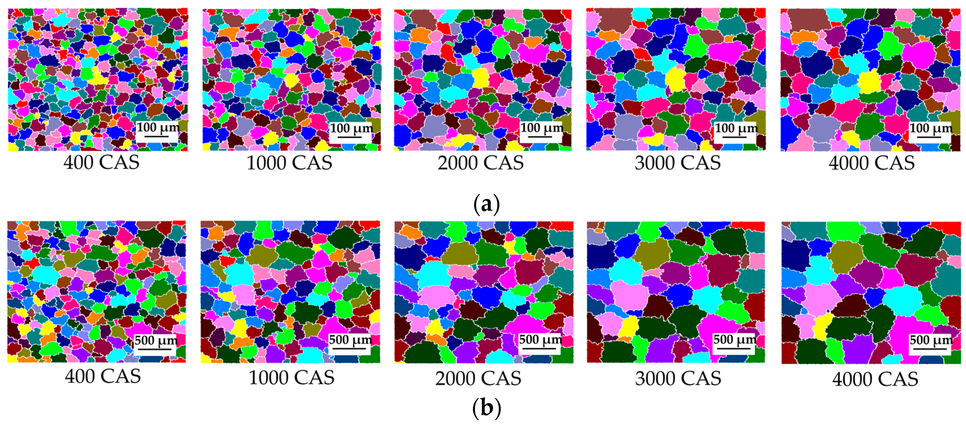
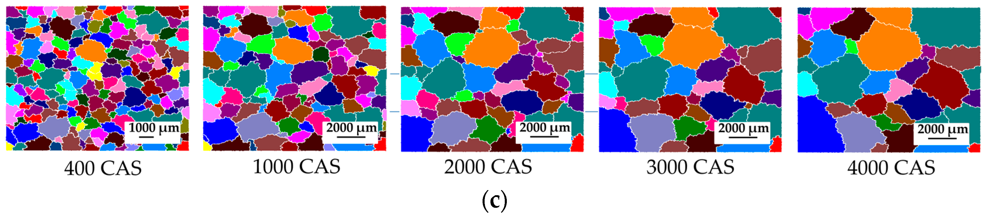
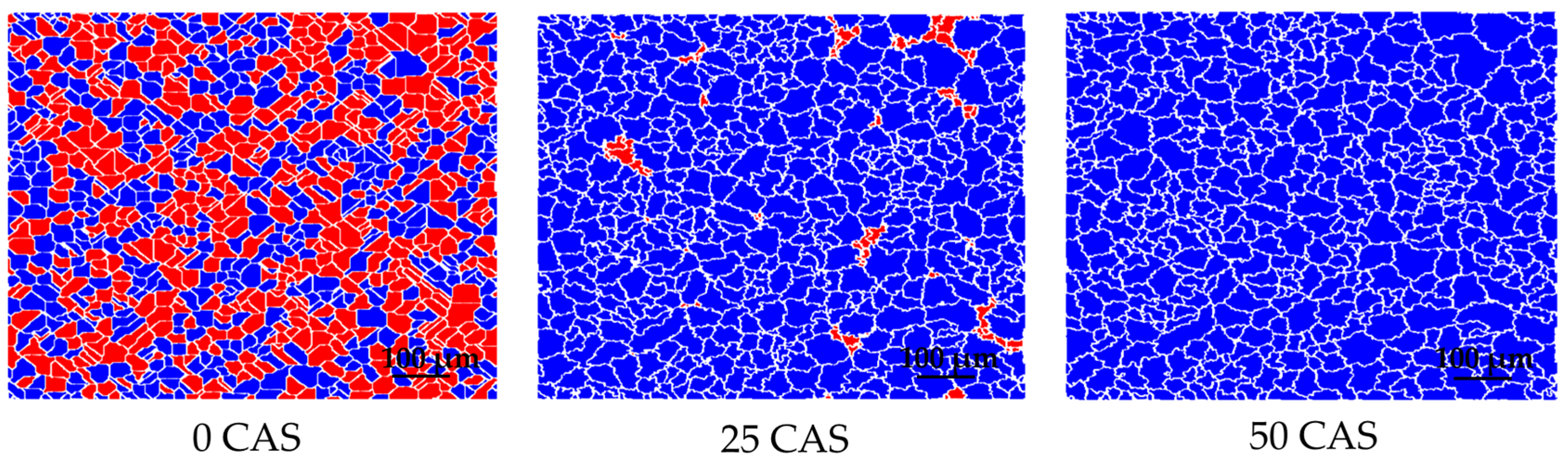
3.2. Microstructure Evolution during the Isothermal Heating

Figure 5 shows the microstructure of the grain growth at different temperatures and Figure 5 shows the microstructure of the grain growth at different temperatures and simulation time calculated by the CA model. The white closed boundary represents the grain boundary, and the interior of the grain is filled with color. Due to the unique orientation of each grain, the grain growth caused by the grain coalescence is avoided, which is inconsistent with the actual situation. Then the grain coarsening is dominated by diffusion at grain boundaries and consumption of smaller grains adjacent to larger grains. The previous studies indicate that if the simulation model of grain growth only considers the lowest energy principle, the calculated grain boundaries are smooth and straight [40]. As the CA model developed in this paper considers the effects of the thermodynamic driving mechanism, the lowest energy principle and curvature-driven mechanism on the grain growth, the homogeneously distributed grains have the polygonal shape with zigzag rather than smooth grain boundaries, which is consistent with the grain growth mechanism. Figure 5 suggests that the grain size increases as the CAS increases at a certain temperature, and the larger temperature leads to a larger average grain size at a certain CAS.

The value of $C$ is used to measure the grain boundary length calculated by Equation (8):

$$C={\displaystyle \sum _j^M(1-{\delta }_{s_i}{\delta }_{s_j})}\times \Delta x={\displaystyle \sum _j^M(1-{\delta }_{s_i}{\delta }_{s_j})}\times \Delta y$$

(8)

Moore neighborhood is adopted to compute the grain boundary length, hence the value of $M$ is 8. The other variables in this equation can be referred to in Equation (6). Figure 6 shows the distribution of two types of grains in the initial microstructure of 25Cr2Ni4MoV steel just reaching 1173 K. The initial Type II-Type II grain boundary length is 21,377, while the total length of Type I-Type I, Type I-Type II and Type II-Type I grain boundaries is 73,498. Therefore, the proportion of Type II-Type II grain boundaries is about 25%, indicating that different types of grain boundaries are uniformly distributed in the initial microstructure. As shown in Figure 6, the total grain boundary length decreases at the condition of 1173 K/25 CAS. The length of the Type II-Type II grain boundary was 79,066, and the ratio of the Type II-Type II grain boundary length to the total grain boundary length rapidly increased to 86.5%. The total length of the Type I-Type I, Type I-Type II, and Type II-Type I grain boundary rapidly decreased to 12,358, and correspondingly its proportion decreased to 13.5%. Although there is anisotropic grain boundary energy in the system at this time, the uniformly distributed grains exhibit normal grain growth. Figure 6 shows the Type I grain and the grain boundaries formed by the Type I grain basically disappear at 50 CAS, and there are mostly Type II-Type II grain boundaries in the system. Therefore, when the temperature is constant, with the extension of the simulation time, only the type of grain boundary with the lowest energy exists in the grain system. Hence, the system presents an isotropic grain growth. Moreover, the higher the temperature, the faster the grains enter the isotropic grain growth. When the temperature is not less than 1273 K and the simulation time is not less than 15 CAS, the anisotropic grain growth considering the anisotropic grain boundary energy disappears and 25Cr2Ni4MoV steel undergoes the isotropic grain growth. This is because the higher the temperature and the longer the holding time, the closer the material is to the equilibrium and homogenization state, and the more likely it is to achieve isotropic grain growth.

In this paper, Beck’s equation is used to calculate the relationship between the average grain size and the simulation time [13]. The grain growth kinetics can be expressed by:

$$\overline{D}=k_1{t}^n$$

(9)

where $\overline{D}$ is the average grain diameter, $t$ is the simulation time, $k_1$ is the constant and $n$ is the growth exponent. The research on the growth exponent has always been controversial. Different simulation methods [41,42,43] and experiments [44,45,46] can obtain different grain growth exponents. Many studies have pointed out that the growth exponent range is $0\le n\le 0.5$ [47,48,49]. When the influence of impurities and second phase particles on normal grain growth can be ignored, the grain growth exponent is usually 0.5. Figure 7 shows the relationship between the average grain diameter and the simulation time at different temperatures. Figure 8 shows the linear relationship between $\ln D$ and $\ln t$. The fitting results are basically consistent with the experimental results as shown in Figure 9. It is determined that the grain growth exponent simulated by the CA model is approximately 0.35 by taking the average slope value. It can be explained that more lattice points are occupied within the grain as the simulation time increases. Due to the strong randomness of the CA method, randomly selected lattice points are more likely to fall within the grain rather than at the grain boundary. Therefore, with the extension of the simulation time the possibility of achieving the grain growth through the grain boundary migration decreases, and the grain growth slows down, resulting in a growth exponent of less than 0.5.

One of the advantages of computer simulations is that the properties of a large number of individual grains can be monitored. Hence the kinetics of individual grains can be studied.

Hillert proposed the relationship between the growth rate of an individual grain and its size as shown in Equation (10) [50]:

$$dR/dt=-k_2\left(1/R-1/R_{cr}\right)$$

(10)

where $k_2$ is a positive coefficient, $R$ is the radius of a given grain. $R_{cr}$ is the critical grain radius. Generally, in two-dimensional systems, the critical radius is equal to the average grain radius ($R_a$).

Figure 10 shows the relationship between the average growth rates and the grain radii by analyzing the results of 2928 grains at different temperatures with different CAS. It is shown that the grains with radii larger than $R_{cr}$ will grow and those with radii less than $R_{cr}$ will shrink, which conforms to the Hillert equation well. However, each individual grain may not follow Hillert’s equation. It is clear that the plot shows a large fluctuation in the data, especially for grains close to the average grain size. Therefore, it is impossible to obtain a linear relationship between the average grain growth rate and the grain radii, which is different from previous research results [22].

As shown in Figure 11, the highest grain size frequency is 34.2% for grains ($1/R-1/R_{cr}=0.00344$) slightly smaller than the average grain size, followed by 32.5% for grains ($1/R-1/R_{cr}=-0.00358$) slightly larger than the average grain size. Apparently, the difference in frequency between these two types of grains is not significant. It indicates that when some grains grow, there will be a corresponding number of grains shrinking, so the grains have grown normally. The frequency of the grain size ($-0.00358\le 1/R-1/R_{cr}\le 0.00344$) near the average value is the highest. Meanwhile, the number of grains ($1/R-1/R_{cr}\le -0.021$) significantly larger than the average grain size is 0, and the number of grains ($1/R-1/R_{cr}\ge 0.067$) significantly smaller than the average grain size is also very small, which also indicates that the grain size distribution is relatively uniform. The growth rate of grains ($1/R-1/R_{cr}=-0.00358$) slightly larger than the average grain size is the highest, while the shrinking rate of grains ($1/R-1/R_{cr}=0.00344$) slightly smaller than the average grain size is the highest. The maximum grain shrinking rate is approximately six times the maximum grain growth rate. This is significantly different from abnormal growth, where the maximum grain growth rate is twice the maximum grain shrinking rate [27], indicating that a few grains have significant growth advantages. Figure 10 and Figure 11 also indicate that the normal grain growth calculated by the CA model is mainly achieved by the grains slightly larger than the average grain size swallowing grains slightly smaller than the average grain size, and the number of two types of grains that undergo significant growth and shrinkage is nearly equal.

Figure 12 shows that there are only a few grains with the grain size smaller than 4 or larger than 9. The 5-sided grains have the highest probability of occurrence nearly among all the topological classes, followed by 6-sided grains, and finally the 4-sided grains. The number of sides with the highest frequency has always been controversial. Some experimental and simulation models show that the value is 5 [51,52], while others indicate that the value is 6 or greater [22,41,53]. Studies have shown that the initial microstructure significantly affects the topology during grain growth [54,55]. Figure 12 shows the highest frequency in the initial microstructure is 5-sided grains, followed by 6-sided grains. This may promote the occurrence of the phenomenon that the frequency of the 5-sided grains rather than the 6-sided grains is the highest during the subsequent grain growth process.

As there are only few grains that have less than 4 sides or more than 9 sides, only the growth kinetics of grains with 4–9 sides were studied. As shown in Figure 13 the area change rate of all grains with a side number of not less than 6 is greater than 0, and the average area change rate of all 4-sided grains is less than 0. Therefore, grains with a side number not less than 6 are growing, while 4-sided grains are shrinking. The situation for 5-sided grains is complicated. Those grains can either grow or shrink as well as have zero growth rate depending on their sizes and their neighbor grains or local topology arrangements. As shown in Figure 14, by taking the average value of the results of all temperatures and step sizes, it is found that the average area change rate is less than 0 for grains with less than 6 sides, while the average area change rate is greater than 0 for grains with no less than 6 sides. However, the area change rate of the 5-sided grain rather than the 6-sided grain is closer to zero, which is inconsistent with the Mullins equation [56]. One of the reasons for this disagreement may be the fact that this equation comes purely from the mathematical requirement of space-filling, and surface tension constraints are not considered. Regardless of the number of sides, the total growth rate is larger than zero for all grains in the system.

Grain size distribution is widely used to study the uniformity of microstructure. Figure 15 shows the grain size distribution at 1523 K with different simulation times. The grain size distribution obeys logarithmic normal distribution at 400 CAS. With the extension of the simulation time, the grain size distribution is not very stable. This instability is mainly due to changes in the number of larger and smaller grains. For example, grains with $0<R/R_m<0.2$ appear at 400 CAS, 1000 CAS and 3000 CAS, while grains with this size disappear at 2000 CAS and 4000 CAS. Then a small number of grains with $R/R_m>2$ appear at 400 CAS and 1000 CAS, which disappear with the increase of the simulation time. The results of all different simulation steps indicate that the maximum frequency is at $R/R_m\approx 0.9\sim 0.1$, which means that most grain sizes are close to the average grain size. When $R/R_m$ approaches 0 or 2, the distribution frequency approaches 0, indicating that there are few grains of larger and smaller sizes than the average grain size and the grain size distribution is relatively uniform. Figure 15 shows that the cutoff positions for 400 CAS and 1000 CAS are 2.1, and the cutoff value for other simulation steps is 1.9. It is close to the cutoff value of 2–2.5 reported in most studies [57,58,59].

4. Conclusions

It is necessary to reveal the grain growth of 25Cr2Ni4MoV steel to optimize the manufacturing process design of the super-large nuclear-power rotor. The grain size of 25Cr2Ni4MoV steel reaches stability when the holding time exceeds 2 h. Then an improved isothermal grain growth model during the isothermal heating process was built by considering the steady-state grain size. Based on the isothermal grain growth model and the rule of additivity, a grain growth model for 25Cr2Ni4MoV steel during the continuous heating process was established. The prediction results of the model are basically consistent with the experimental results, indicating the grain growth models for a common heating process including continuous heating and isothermal heating have good predictability.

The CA model considering anisotropic grain boundary energy based on the thermodynamic driving mechanism, curvature-driven mechanism and the lowest energy principle has been established to simulate the grain growth during the isothermal heating process of 25Cr2Ni4MoV steel. The CA simulation shows that the grains have a polygonal shape with zigzag rather than smooth grain boundaries. Among the grains with different sides, 5-sided grains have the highest frequency, followed by 6-sided grains. The local growth kinetics shows that the relationship between the area change rate and the grain side is inconsistent with the Mullins equation, as the average area change rate of the 5-sided grains rather than the 6-sided grains is closer to zero.

The grain size distribution shows a maximum frequency of $R/R_m$ is 0.9–1.1. When $R/R_m$ approaches 0 or 2, the distribution frequency approaches 0, indicating the grain size distribution is relatively uniform. The kinetics of normal grain growth follows Beck’s equation and the growth exponent is 0.35, and the relationship between grain growth rates and grain radii is not linear. It is found that the normal grain growth of 25Cr2Ni4MoV steel is mainly achieved by the grains slightly larger than the average grain size swallowing grains slightly smaller than the average grain size, and the number of two types of grains that, respectively, experiencing significant growth and shrinkage is nearly equal.

The energy variance of the grain growth of 25Cr2Ni4MoV steel during the isothermal heating process is explained by the present CA model considering anisotropic grain boundary energy. The anisotropic grain growth of 25Cr2Ni4MoV steel considering anisotropic grain boundary energy mainly exists at the early stage of the isothermal heating process with lower temperatures, and the normal grain growth occurs under anisotropic grain boundary energy conditions. The anisotropic grain boundary energy disappears faster with the increasing temperature and holding time. According to the CA model, when the temperature is not less than 1273 K and the CAS is not less than 15 CAS, the normal grain growth containing only isotropic grain boundary energy occurs. The analysis of the morphology, energy variance, topology, grain growth kinetics and grain size distribution indicates that the normal grain growth of 25Cr2Ni4MoV steel can be simulated fairly well by the present CA model.

References

1. Chen, F.; Ren, F.C.; Cui, Z.S. Constitutive modeling for elevated temperature flow behavior of 30Cr2Ni4MoV ultra-super-critical rotor steel. J. Iron Steel Res. Int. 2014, 21, 521–526. [Google Scholar] [CrossRef]
2. Luo, L.; Huang, Y.; Weng, S.; Xuan, F.Z. Mechanism-related modelling of pit evaluation in the CrNiMoV steel in simulated environment of low pressure nuclear steam turbine. Mater. Des. 2016, 105, 240–250. [Google Scholar] [CrossRef]
3. Gong, H.; Guo, Z.; Liu, J.S. Growth behavior of austenite grain of forged 12%Cr ultra-supercritical rotor steel. Heat Treat. Met. 2017, 42, 215–219. [Google Scholar]
4. Li, W.; Liang, C.; Zhang, X. Numerical simulation of microstructure evolution of high-purity tantalum during rolling and annealing. Model Simul. Mater. Sci. 2022, 30, 035006. [Google Scholar] [CrossRef]
5. Salvalaglio, M.; Srolovitz, D.J.; Han, J. Disconnection-Mediated migration of interfaces in microstructures: Ⅱ. diffuse interfaces simulations. Acta Mater. 2022, 227, 117463. [Google Scholar] [CrossRef]
6. Liu, H.G.; Xu, X.; Zhang, J.; Liu, Z.C.; He, Y.; Zhao, W.H.; Liu, Z.Q. The state of the art for numerical simulations of the effect of the microstructure and its evolution in metal-cutting processes. Int. J. Mach. Tools Manuf. 2022, 177, 103890. [Google Scholar] [CrossRef]
7. Fang, X.S.; Wang, P.P.; Xi, T.T.; Sui, F.L.; Qiao, B. Analysis on upsetting and stretching process of 25Cr2NI4MoV steel for heavy forgings. J. Plast. Eng. 2022, 29, 47–55. [Google Scholar]
8. Ye, L.Y.; Zhai, Y.W.; Zhou, L.Y.; Wang, H.Z.; Jiang, P. The hot deformation behavior and 3D processing maps of 25Cr2Ni4MoV steel for a super-large nuclear-power rotor. J. Manuf. Process 2020, 59, 535–544. [Google Scholar] [CrossRef]
9. Ye, L.Y.; Zhai, Y.W.; Zhou, L.Y.; He, X.M. Study on static grain growth of 25Cr2Ni4MoV steel for super large nuclear power rotor. J. Plast. Eng. 2021, 28, 146–151. [Google Scholar]
10. Jiao, S.; Penning, J.; Leysen, F.; Houbaert, Y.; Aernoudt, E. The modeling of the grain growth in a continuous reheating process of a low carbon Si-Mn bearing TRIP steel. ISIJ Int. 2000, 40, 1035–1040. [Google Scholar] [CrossRef]
11. Anelli, E. Application of mathematical modelling to hot rolling and controlled cooling of wire rods and bars. ISIJ Int. 1992, 32, 440–449. [Google Scholar] [CrossRef]
12. Jiang, B.; Zhou, L.Y.; Wen, X.L.; Zhang, C.L.; Liu, Y.Z. Prediction model for the austenite grian growth in medium carbon alloy steel 42CrMo. Metall. Res. Technol. 2014, 111, 369–374. [Google Scholar]
13. Beck, P.A.; Holzworth, M.L.; Hu, H. Instantaneous rates of grain growth. Phys. Rev. 1948, 73, 526–527. [Google Scholar] [CrossRef]
14. Sellars, C.M.; Whiteman, J.A. Recrystallization and grain growth in hot rolling. Met. Sci. 1979, 13, 187–194. [Google Scholar] [CrossRef]
15. Devadas, C.; Samarasekera, I.V.; Hawbolt, E.B. The thermal and metallurgical state of steel strip duirng hot rolling: Part III: Microstructure evolution. Metall. Trans. A 1991, 22, 335–349. [Google Scholar] [CrossRef]
16. Kotan, H.; Darling, K.A. Isothermal annealing of a thermally stabilized Fe-based ferritic alloy. J. Mater. Eng. Perform. 2015, 24, 3271–3276. [Google Scholar] [CrossRef]
17. Jin, Q.L. Constitutive relation for huge forgings. J. Plast. Eng. 2012, 19, 1–10. [Google Scholar]
18. Xiong, F.Y.; Huang, C.Y.; Kafka, O.L.; Lian, Y.P.; Yan, W.T.; Chen, M.J.; Fang, D.N. Grain growth prediction in selective electron beam melting of Ti-6Al-4V with a cellular automaton method. Mater. Des. 2020, 199, 109410. [Google Scholar] [CrossRef]
19. Chen, Z.K.; Li, X.Y. Numerical simulations for microstructure evolution during metal additive manufacturing. Adv. Mech. 2022, 52, 398–407. [Google Scholar]
20. Wen, Z. Three-dimensional cellular automaton simulation of austenite grain growth of Fe-1C-1.5Cr alloy steel. J. Mater. Res. Technol. 2020, 9, 180–187. [Google Scholar]
21. Chen, F.; Zhu, H.J.; Li, J.H.; Cui, Z.S. Macro and micro simulation of microstructure evolution in discontinuous thermal deformation of large forgings parts. J. Plast. Eng. 2020, 27, 41–52. [Google Scholar]
22. He, Y.Z.; Ding, H.L.; Liu, L.F.; Shin, K.S. Computer simulation of 2D grain growth using a cellular automata model based on the lowest energy principle. Mater. Sci. Eng. A 2006, 429, 236–246. [Google Scholar] [CrossRef]
23. Suwa, Y.; Ushioda, K. Phase-field simulation of abnormal grain growth due to the existence of second-phase particles. ISIJ Int. 2022, 62, 577–585. [Google Scholar] [CrossRef]
24. Hu, J.F.; Wang, X.H.; Zhang, J.Z.; Luo, J.; Zhang, Z.J.; Shen, Z.J. A general mechanism of grain growth-I. Theory. J. Materiomics 2021, 7, 1007–1013. [Google Scholar] [CrossRef]
25. Zollner, D.; Sandim, H.R.Z. Abnormal grain growth in thin wires of commercially pure iron with anisotropic microstructure. J. Mater. Res. Technol. 2020, 9, 11099–11110. [Google Scholar]
26. Kinoshita, T.; Ohno, M. Phase-field simulation of abnormal grain growth during carburization in Nb-added steel. Comp. Mater. Sci. 2020, 177, 109558. [Google Scholar] [CrossRef]
27. Ye, L.Y.; Mei, B.Z.; Yu, L.M. Modeling of abnormal grain growth that considers anisotropic grain boundary energies by cellular automaton model. Metals 2022, 12, 1717. [Google Scholar] [CrossRef]
28. Mohapatra, S.; Prasad, R.; Jain, J. Temperature dependence of abnormal grain growth in pure magnesium. Mater. Lett. 2021, 283, 128851. [Google Scholar] [CrossRef]
29. Li, X.; Zhou, Q.; Chen, M.H.; Wang, X.F. Cellular automata simulation for grain growth based on anisotropic grain boundary mobility and grain boundary energy. Mater. Mech. Eng. 2012, 36, 82–92. [Google Scholar] [CrossRef]
30. Wang, H.; Zhang, J.S.; Zong, X.M.; Niu, X.F.; Xu, C.X.; Zhao, D.W. Computer simulation of grain growth with anisotropy grain boundary energy. Mater. Technol. 2014, 3, 44–46. [Google Scholar] [CrossRef]
31. Kotan, H.; Darling, K.A.; Saber, M.; Scattergood, R.O.; Koch, C.C. An in situ experimental study of grain growth in a nanocrystalline Fe91Ni8Zr1. J. Mater. Sci. 2013, 48, 2251–2257. [Google Scholar] [CrossRef] [Green Version]
32. Dake, J.M.; Krill, C.E. Sudden loss of thermal stability in Fe-based nanocrystalline alloys. Scr. Mater. 2012, 66, 390–393. [Google Scholar] [CrossRef]
33. Schuh, B.; Pippan, R.; Hohenwarter, A. Tailoring bimodal grain size structures in nanocrystalline compositionally complex alloys to improve ductility. Mater. Sci. Eng. A 2019, 748, 379–385. [Google Scholar] [CrossRef]
34. Rollett, A.D.; Srolovitz, D.J.; Anderson, M.P. Simulation and theory of abnormal grain growth-anisotropic grain boundary energies and mobilities. Acta Metall. 1989, 37, 1227–1240. [Google Scholar] [CrossRef] [Green Version]
35. Wang, M.; Yin, Y.J.; Zhou, J.X.; Nan, H.; Wang, T.; Li, W. Cellular automata simulation for high temperature austenite grain growth based on thermal activation theory and curvature-driven mechanism. Can. J. Phys. 2016, 94, 1353–1364. [Google Scholar] [CrossRef] [Green Version]
36. Liu, Y.X.; Ke, Z.J.; Li, R.H.; Song, J.Q.; Ruan, J.J. Study of grain growth in a Ni-based superalloy by experiments and cellular automaton model. Materials 2021, 14, 6922. [Google Scholar] [CrossRef]
37. Raghavan, S.; Sahay, S.S. Modeling the grain growth kinetics by cellular automaton. Mater. Sci. Eng. A 2007, 445, 203–209. [Google Scholar] [CrossRef]
38. Han, F.B.; Tang, B.; Kou, H.C.; Li, J.S.; Feng, Y. Cellular automata simulations of grain growth in the presence of second-phase particles. Model. Simul. Mater. Sci. Eng. 2015, 23, 065010. [Google Scholar] [CrossRef]
39. Doherty, R.D.; Huges, D.A.; Humphreys, F.J.; Jonas, J.J.; Jensen, D.J.; Kassner, M.E.; King, W.E.; McNElley, T.R.; McQueen, H.J.; Rollet, A.D. Current issues in recrystallization: A review. Mater. Sci. Eng. A 1997, 238, 219–274. [Google Scholar] [CrossRef] [Green Version]
40. Srolovitz, D.J.; Anderson, M.P.; Sahni, P.S. Computer simulation of grain growth—II. Grain size distribution, topology, and local dynamics. Acta Metall. 1984, 32, 793–802. [Google Scholar] [CrossRef]
41. Kim, B.N.; Hiraga, K.; Morita, K. Kinetics of normal grain growth depending on the size distribution of small grains. Mater. Trans. 2003, 44, 2239–2244. [Google Scholar] [CrossRef] [Green Version]
42. Yu, Q.; Esche, S.K. A new perspective on the normal grain growth exponent obtained in two-dimensional Monte Carlo simulations. Model. Simul. Mater. Sci. Eng. 2003, 11, 859–861. [Google Scholar] [CrossRef]
43. Zheng, Y.; Song, J.L. Cellular automata simulation of austenite grain growth for LZ50 steel. J. Plast. Eng. 2015, 22, 141–147. [Google Scholar]
44. Holmes, E.L.; Winegard, W.C. Grain growth in zone-refined tin. Acta Metall. 1959, 7, 411–414. [Google Scholar] [CrossRef]
45. Petrovic, V.; Ristic, M.M. Isochronal and isothermal grain growth during sintering of Cadmium Oxide. Metallography 1980, 13, 319–327. [Google Scholar] [CrossRef]
46. Ji, H.P.; Guo, B.F.; Liu, X.G.; Zhang, L.G.; Jin, M. Application of cellular automata in grain growth simulation of 316LN stainless steel. J. Yanshan Univ. 2013, 37, 389–395. [Google Scholar]
47. Anderson, M.P.; Grest, G.S. Computer simulation of normal grain growth in three dimensions. Philos. Mag. Part B 1989, 59, 293–329. [Google Scholar] [CrossRef]
48. Holm, E.A.; Zacharopoulos, N.; Srolovitz, D.J. Nonuniform and directional grain growth caused by grain boundary mobility variations. Acta Mater. 1997, 46, 953–964. [Google Scholar] [CrossRef]
49. Rhines, F.N.; Craig, K.R.; Dehoff, R.T. Mechanism of steady-state grain growth in aluminum. Metall. Trans. 1974, 5, 413–425. [Google Scholar] [CrossRef]
50. Hillert, M. On the theory of normal and abnormal grain growth. Acta Metall. 1965, 13, 227–238. [Google Scholar] [CrossRef]
51. Fan, D.; Geng, C.W.; Chen, L.Q. Computer simulation of topological evolution in 2-D grain growth using a continuum diffuse-interface field model. Acta Mater. 1997, 45, 1115–1126. [Google Scholar] [CrossRef]
52. Glazier, J.A.; Anderson, M.P.; Grest, G.S. Coarsening in the two-dimensional soap froth and the large-Q Potts model: A detailed comparison. Philos. Mag. B Phys. Condens. Matter 1990, 62, 615–645. [Google Scholar]
53. Yu, Q.; Esche, S.K. Modeling of grain growth kinetics with Read-Shockley grain boundary energy by a modified Monte Carlo algorithm. Mater. Lett. 2002, 56, 47–52. [Google Scholar] [CrossRef]
54. Gao, J.B.; Wei, M.; Zhang, L.J.; Du, Y.; Liu, Z.M.; Huang, B.Y. Effect of different initial structures on the simulation of microstructure evolution during normal grain growth via phase-field modeling. Metall. Mater. Trans. A Phys. Metall. Mater. Sci. 2018, 49, 6442–6456. [Google Scholar] [CrossRef]
55. Li, J.; Huang, J.; Jia, T. Effect of initial microstructure on austenite transformation and grain growth behavior of 20CrMnTi steel during pseudo-carburizing process. Heat Treat. Met. 2020, 45, 157–162. [Google Scholar]
56. Mullins, W.W. Two-dimensional motion of idealized grain boundaries. J. Appl. Phys. 1956, 27, 900–904. [Google Scholar] [CrossRef]
57. Xia, Z.Y.; Chen, R.C.; Hong, C.; Zheng, Z.Z.; Li, J.J. Cellular automata simulation of grain growth during heat preservation for 300M steel. J. Plast. Eng. 2018, 25, 73–79. [Google Scholar]
58. Song, X.; Liu, G.; Nanju, G. Re-analysis on grain size distribution during normal grain growth based on monte carlo simulation. Scr. Mater. 2000, 43, 355–359. [Google Scholar]
59. Jin, Z.Y.; Yu, D.H.; Wu, X.T. Simulation of grain growth behavior of hot-extruded pure magnesium by cellular automata. J. Plast. Eng. 2016, 23, 209–215. [Google Scholar]
Figure 1. The relationship between A C 1 temperature, A C 3 temperature, the homogeneous temperature and the heating rate of 25Cr2Ni4MoV steel.
Metals 13 01072 g001
Figure 2. The flowchart of the calculation procedure of the grain size in the continuous heating process.
Metals 13 01072 g002
Figure 3. The comparison of the experimental and calculated austenite grain size.
Metals 13 01072 g003
Figure 4. The flowchart of the CA model for austenite grain growth in the isothermal heating process.
Metals 13 01072 g004
Figure 5. Microstructure evolution at different temperatures with different simulation time. (a) Microstructure evolution at 1173 K with different simulation time (CAS is equal to the number of program cycles divided by the grid size, and the grid size is 500 × 500 ). (b) Microstructure evolution at 1373 K with different simulation time. (c) Microstructure evolution at 1523 K with different simulation time.
Metals 13 01072 g005aMetals 13 01072 g005b
Figure 6. The distribution of two types of grains at 1173 K with different time (The red filled area represents Type I grains, while the blue filled area represents Type II grains).
Metals 13 01072 g006
Figure 7. The relationship between the average grain diameter and the simulation time.
Metals 13 01072 g007
Figure 8. The relation between average grain diameter ( ln D ¯ ) and time ( ln t ) during grain growth.
Metals 13 01072 g008
Figure 9. The comparison of the experimental and fitting grain size for grain growth.
Metals 13 01072 g009
Figure 10. Average data for grain growth rate d R / d t in grain size ( 1 / R 1 / R c r ) space. The data were averaged with the interval Δ ( 1 / R 1 / R c r ) = 0.01 .
Metals 13 01072 g010
Figure 11. The distribution of grain size ( 1 / R 1 / R c r ).
Metals 13 01072 g011
Figure 12. The distribution of the grain side ( n ) at different temperatures.
Metals 13 01072 g012
Figure 13. The relationship between the growth rate ( d A / d t , A is the grain area of all the grains with the same number of grain side) and the simulation time at different grain sides ( n ).
Metals 13 01072 g013
Figure 14. The dependence of the average growth rate ( d A n / d t ) on number of grain side ( n ).
Metals 13 01072 g014
Figure 15. The grain size distribution at 1523 K with different simulation time.
Metals 13 01072 g015