Dynamic Modeling and Stability Prediction of Robot Milling Considering the Influence of Force-Induced Deformation on Regenerative Effect and Process Damping

Abstract

Undesirable chatter is one of the key problems that restrict the improvement of robot milling quality and efficiency. The prediction of chatter stability, which is used to guide the selection of process parameters, is an effective method to avoid chatter in robot milling. Due to the weak stiffness of the robot, deformation caused by milling forces becomes an unavoidable problem, which will change the tool–workpiece contact area and affect the stability prediction. However, it is often simplified and neglected. In this paper, a multipoint contact dynamic model of robot milling is established, which considers the influence of force-induced deformation on the regenerative effect and process damping. The tool–workpiece contact area is discretized into a finite number of nodes along the axial direction so that the force and deformation at each node can be calculated separately. The different contact forms of the tool–workpiece under different process parameters are discussed in different cases, and the interaction process between cutting force and force-induced deformation is analyzed in detail. An iterative strategy is used to calculate the deformation of each node and the result of the tool–workpiece contact boundary. Finally, chatter stability of robot milling is predicted by a fully discrete method. Robot milling experiments were carried out to verify the predicted results. The results show that force-induced deformation is an important factor improving the stability prediction accuracy of robot milling, and a more accurate prediction result can be obtained by simultaneously considering force-induced deformation and process damping.

1. Introduction

Industrial robots are desired to be applied in the machining of large complex parts due to the advantages of low cost and high efficiency [1,2,3,4]. Previous research has shown that robot machining can save significant costs and provide greater flexibility compared to CNC machine tools [5,6,7]. However, the machining chatter caused by the low stiffness of the robot, which leads to the rapid wear of the tool and the deterioration of the machining quality, is one of the main problems restricting the application of robots to high-load processing (especially milling) [8,9,10]. Therefore, the chatter problem of robot milling deserves special attention. Research shows that the prediction of the stable lobe diagram (SLD) can guide the selection of process parameters, and it is an effective method to avoid chatter [11]. Therefore, several methods for predicting SLD have been developed.

Over the past three decades, many methods have been proposed for predicting SLD [12], such as zero-order approximation (ZOA) [13,14,15], multi-frequency method (MFM) [16,17], semi-discretization method (SDM) [18,19] and full-discretization method (FDM) [20]. Based on the above methods, many scholars have predicted the SLD of robot milling. Mousavi et al. [21,22] established the robot dynamics model by the multi-body dynamics method, and then based on the regenerative chatter theory, the robot kinematic redundancy was used as a function variable to obtain the SLD. Gonul et al. [23] identified the dynamic parameters of the robot milling system under different postures, and the SLD of robot milling was predicted by the frequency domain method. Cordes et al. [24] established the structural dynamics model of the robot milling system, and SLD was predicted by the frequency domain method and SDM method. Mejri et al. [25] used the single frequency method to predict the SLD of robot milling and studied the influence law of the posture change on the robot milling stability. The above studies on robot milling chatter focus on the use of accurate SLD prediction algorithms, and are less concerned with the accuracy of robot milling dynamics modeling.

Research shows that in addition to adopting accurate SLD prediction algorithms, much effort is also needed to construct an accurate milling dynamic model to improve the prediction accuracy of SLD [26]. Xin et al. [27] found that robot milling chatter is affected by tool point low-frequency vibration, which is caused by robot structure mode, and established the stability prediction model considering the tool point low-frequency vibration caused by robot structure mode. The experimental results show that considering the low frequency vibration of the robot can improve the prediction accuracy of SLD at low milling speed. Li et al. [28] established a two-degree-of-freedom robot milling dynamics model considering the effect of structure mode coupling, which can obtain a more accurate SLD for robot milling. Mohammadi et al. [29] took the nonlinear cutting force caused by the axial vibration of the robot into the milling dynamics model, which improved the prediction accuracy of SLD. Wang et al. [30] established a multiple degrees of freedom dynamic equation simultaneously considering the robot mode and tool mode, which improved the prediction accuracy of SLD in robot milling at a low tool rotation speed. In conclusion, the construction of a more accurate milling dynamics model can effectively improve the prediction accuracy of SLD for robot milling. When studying machining chatter in CNC machining centers, some studies have shown that force-induced deformation can cause the actual radial cutting depth to be different from the nominal one, which can lead to a change in milling stability. For example, Sun et al. [31] studied the effect of force-induced deformation on the milling stability in the machining center, and constructed a dynamics model in milling thin-walled part considering force-induced deformation effect, which can improve the prediction accuracy of SLD. Considering the series structure characteristic of the robot, the flexible characteristics of robot joints will inevitably cause force-induced deformation in the milling process, and its influence on the stability of robot milling cannot be ignored.

In order to further consider the robot milling deformation factor in the chatter stability prediction model, an iterative calculation strategy for milling deformation is proposed in this paper. This strategy takes into account the different contact states between tool and workpiece, which realizes the calculation of milling deformation under different process parameters. Furthermore, a multipoint contact dynamic model considering regeneration effect and process damping is constructed, and the calculated milling deformation is taken into account. A fully discrete method is applied to predict the SLD of robot milling and the stability prediction results show that compared with the traditional model, the predicted stability area is further expanded by considering milling deformation and process damping. Especially at the peak of SLD, the expansion is larger. For example, when the spindle speed is 8200 rpm, compared with the traditional model, the stability boundary is increased by 25% after considering deformation and process damping. The predicted expansion region is also verified as the stable region by the experiment, which shows the correctness of the model. The research provides theoretical guidance for the stability prediction of robot milling.

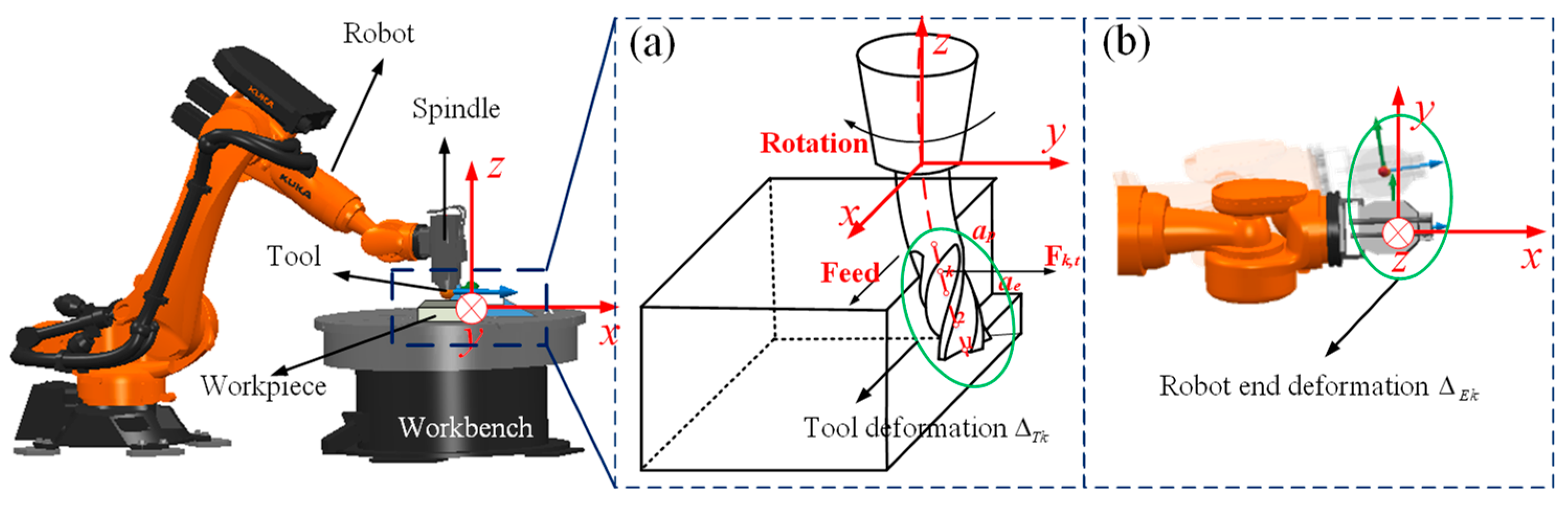
2. Analysis of Force-Induced Deformation in Robot Milling

In the milling process, the robot milling system (KUKA, Augsburg, Germany) is usually considered as the flexible part, while the workpiece is considered as the rigid part. Therefore, the force-induced deformation of robot milling can be divided into two parts: tool deflection deformation and robot joint deformation. Schematic Figure 1 shows the deformation principle in the process of robot milling with an end mill. Figure 1a shows the variation of tool deformation along the tool axis due to the influence of tool deflection. The tool is divided into m elements along the axis, and the deformation of each element node can be calculated separately [31,32,33,34], which can be expressed as follows:

$${\Delta }_{\mathrm{T}}(k,n)=\{\begin{array}{cc}\frac{{\mathit{F}}_n\cdot {(l-z_k)}^2}{6EI}(2l-3z_n+z_k)& z_n<z_k<l\\ \frac{{\mathit{F}}_n\cdot {(l-z_n)}^2}{6EI}(2l-3z_k+z_n)& 0<z_k<z_n\end{array}$$

(1)

$${\Delta }_{\mathrm{T}k}={\displaystyle \sum _{n=1}^{m+1}{\Delta }_{\mathrm{T}}(k,n)}$$

(2)

in which ${\mathbf{\Delta }}_{\mathrm{T}}\left(k,n\right)$ represents the deformation of the k-th node caused by the force on the n-th node and ${\mathbf{\Delta }}_{\mathrm{T}k}$ represents the total tool deflection deformation at node k, F_n represents the force on the n-th node, l represents overhang length of tool, z_k represents the distance between the k-th node and the free end of the tool, E represents Young’s modulus of the tool and I represents area moment of inertia.

The deformation of robot joints can be transformed into the deformation of robot end by matrix transformation, as shown in Figure 1b. ${\mathbf{\Delta }}_{\mathrm{E}k}$ represents the deformation of the robot end at axial element node k, which can be calculated as follow:

$${\Delta }_{\mathrm{E}k}={\mathit{J}}_{\mathrm{c}}{{\mathit{K}}_{\mathrm{q}}}^{-1}{{\mathit{J}}_{\mathrm{e}}}^{\mathit{T}}\mathit{F}$$

(3)

where J_c is the velocity Jacobian matrix of the robot, and ${{\mathit{J}}_e}^{\mathit{T}}$ is the force Jacobian matrix of the robot. The robot Jacobian matrix can be derived from a robot kinematic model by using the method proposed by [35]. ${\mathit{K}}_{\mathrm{q}}$ is the diagonal stiffness matrix in the joint coordinate system, which is identified by static payload experiment. F is the resultant force of each element in the milling process.

Therefore, the total deformation of robot milling at axial element node k can be expressed as:

$${\Delta }_{\mathrm{R}k}={\Delta }_{\mathrm{T}k}+{\Delta }_{\mathrm{E}k}$$

(4)

where ${\Delta }_{\mathrm{R}k}$ represents the total deformation of the robot milling system at axial element node k.

3. Dynamic Modeling of Robot Milling

3.1. Multipoint Contact Dynamic Equation

According to the deformation analysis of the robot milling system, the force-induced deformation is calculated at each node along the axial direction of the tool–workpiece contact area. Therefore, the dynamics model of robot milling is considered as a multipoint contact dynamic model, which can simultaneously consider force-induced deformation in the milling stability. The multipoint contact dynamic model can be formulated in physical space as:

$$\mathit{M}\ddot{\mathit{Q}}+\mathit{C}\dot{\mathit{Q}}+\mathit{K}\mathit{Q}=\mathit{F}(t)$$

(5)

where M, C and K stand for 2 (m + 1) × 2(m + 1) dimensional physical mass, damping and stiffness matrices of the robot milling system, $\mathit{F}\left(t\right)$ is the 2 (m + 1) × 1 dimensional cutting force vector. The milling force can be expressed as Equation (6) [31].

$$\mathit{F}(t)={\left[\begin{array}{ccccc}{\mathit{F}}_1(t)& \cdots & {\mathit{F}}_k(t)& \cdots & {\mathit{F}}_{m+1}(t)\end{array}\right]}^T$$

(6)

in which ${\mathit{F}}_k\left(t\right)$ represents the contact force at any node k. In this study, the two degrees of freedom (x-direction and y-direction) are considered at different nodes during side milling as shown in Figure 2. Therefore, the milling force of each node k can be expressed as:

$${\mathit{F}}_k(t)={\left[\begin{array}{cc}{F}_{k,x}(t)& F_{k,y}(t)\end{array}\right]}^T$$

(7)

3.2. Tool–Workpiece Interaction Force

The milling force of each node can be decomposed into static force, process damping force and regenerative dynamic force unit, which can be expressed as follow:

$${\mathit{F}}_k(t)={\displaystyle \sum _{j=1}^N\left[{\mathit{F}}_{j,k}^{\mathrm{s}}(t)+{\mathit{F}}_{j,k}^{\mathrm{c}}(t)+{\mathit{F}}_{j,k}^{\mathrm{d}}(t)\right]}$$

(8)

where N is the number of the tool teeth, and the upper corner subscripts s, c and d represent static, process damping and regenerative dynamic, respectively. The static cutting force causes deformation; process damping force and dynamic milling force affect milling stability [31,36]. ${\mathit{F}}_k\left(t\right)$ can be further decomposed in the x and y directions, as shown in Figure 2. It can be expressed as follow:

$${\mathit{F}}_{j,k}(t)=g_{j,k}^{\mathrm{n}}\left[\begin{array}{c}{F}_{j,k,x}(t)\\ F_{j,k,y}(t)\end{array}\right]=g_{j,k}^{\mathrm{n}}\left[\begin{array}{cc}\sin {\phi }_{j,k}(t)& -\cos {\phi }_{j,k}(t)\\ \cos {\phi }_{j,k}(t)& \sin {\phi }_{j,k}(t)\end{array}\right]\left[\begin{array}{c}{F}_{j,k,t}(t)\\ F_{j,k,r}(t)\end{array}\right]$$

(9)

where ${\phi }_{j,k}\left(t\right)$ represents the engagement angle on the k-th axial node of the j-th tooth between the tool and the workpiece at time t. It can be expressed as:

$${\phi }_{j,k}(t)=\frac{2\pi \Omega }{60}t-(j-1)\frac{2\pi }{N}-k\Delta \varphi$$

(10)

$$\Delta \varphi =\frac{dz\tan \beta }{R}$$

(11)

where $\Omega$ is the rotation speed of the tool, and R is the radius of the tool. dz is the height of the discrete axial element, which can be calculated by $dz=\frac{a_p}{m}$ [31]. $g_{j,k}^{\mathrm{n}}$ is the nominal judgment equation of the milling process, which determines whether the j-th tool tooth participates in cutting.

$$g_{j,k}^{\mathrm{n}}=\{\begin{array}{cc}1& {\phi }_{\mathrm{en},k}^{\mathrm{n}}\le {\phi }_{j,k}(t)\le {\phi }_{\mathrm{ex},k}^{\mathrm{n}}\\ 0& \mathrm{otherwise}\end{array}$$

(12)

in which ${\phi }_{\mathrm{en},k}^{\mathrm{n}}$ and ${\phi }_{\mathrm{ex},k}^{\mathrm{n}}$ represent the nominal entry angle and exit angle of the tool–workpiece contact area, respectively. $F_{j,k,t}\left(t\right)$ and $F_{j,k,r}\left(t\right)$ represent the tangential and radial milling forces on the k-th axial node of the j-th tooth at time t, which can also be decomposed into static force, process damping force and regenerative dynamic force unit. The static force and regenerative dynamic force can be expressed as follows:

$$\{\begin{array}{c}{F}_{j,k,t}^{\mathrm{s}}(t)=g_{j,k}^{\mathrm{n}}\left[K_{\mathrm{tc}}{h}_{j,k}^{\mathrm{s}}(t)+K_{\mathrm{te}}\right]dz\\ F_{j,k,r}^{\mathrm{s}}(t)=g_{j,k}^{\mathrm{n}}\left[K_{\mathrm{rc}}{h}_{j,k}^{\mathrm{s}}(t)+K_{\mathrm{re}}\right]dz\end{array}$$

(13)

$$\{\begin{array}{c}{F}_{j,k,t}^{\mathrm{d}}(t)=g_{j,k}^{\mathrm{n}}\left[K_{\mathrm{tc}}{h}_{j,k}^{\mathrm{d}}(t)\right]dz\\ F_{j,k,r}^{\mathrm{d}}(t)=g_{j,k}^{\mathrm{n}}\left[K_{\mathrm{rc}}{h}_{j,k}^{\mathrm{d}}(t)\right]dz\end{array}$$

(14)

where $K_{\mathrm{tc}}$ and $K_{\mathrm{rc}}$ represent the milling force coefficient contributed by shear effect, $K_{\mathrm{te}}$ and $K_{\mathrm{re}}$ represent the milling force coefficient contributed by plough effect. $h_{j,k}^{\mathrm{s}}\left(t\right)$ and $h_{j,k}^{\mathrm{d}}\left(t\right)$ represent the static and dynamic instantaneous undeformed cutting thickness, which can be approximated as:

$$h_{j,k}^{\mathrm{s}}(t)=f_z\cos {\phi }_{j,k}(t)$$

(15)

$$h_{j,k}^{\mathrm{d}}(t)=\Delta x_{j,k}(t)\cos {\phi }_{j,k}(t)-\Delta y_{j,k}(t)\sin {\phi }_{j,k}(t)$$

(16)

in which $f_z$ is the feed per tooth. Δx_j,k(t) and Δy_j,k(t) are the dynamic displacements of the tool in the x and y directions caused by the regeneration effect. They can be expressed as Equation (17):

$$\{\begin{array}{c}\Delta x_{j,k}(t)=x_{j,k}(t)-x_{j,k}(t-T)\\ \Delta y_{j,k}(t)=y_{j,k}(t)-y_{j,k}(t-T)\end{array}$$

(17)

In this study, the process damping force is established as the equivalent linear viscous damper model proposed by Ahmadi et al. in [36], as shown in Equation (18):

$$\left[\begin{array}{c}{F}_{j,k,t}^{\mathrm{c}}(t)\\ F_{j,k,r}^{\mathrm{c}}(t)\end{array}\right]=g_{j,k}^{\mathrm{n}}{C}_{\mathrm{eq}}\left[\begin{array}{c}\mu \\ 1\end{array}\right]\left[\begin{array}{c}\cos {\phi }_{j,k}(t)-\sin {\phi }_{j,k}(t)\end{array}\right]\left[\begin{array}{c}{\dot{x}}_{j,k}(t)\\ {\dot{y}}_{j,k}(t)\end{array}\right]$$

(18)

where $\mu$ is the Coulomb friction coefficient, which is 0.3. $C_{\mathrm{eq}}$ is the term related to the indentation force, which can be expressed as:

$$C_{\mathrm{eq}}=\frac{K_{sp}{w}^{2}dz}{4v}$$

(19)

where $K_{sp}$ is the indentation force coefficient, which is set as 1.5 × 10¹⁴ N/m³ according to Ref [37], $w$ is the wear band width of cutting edge, which is 40 μm according to the measurement results of the 3D laserscanning microscope (VK-X100, Keyence Co., Ltd., Osaka, Japan), and $v$ is the tangential velocity of the tool, which can be calculated by $v=\frac{2\pi R\Omega }{60}$.

4. Calculation Method of Force-Induced Deformation

4.1. Effect of Force-Induced Deformation on Robot Milling Stability

The effect of force-induced deformation on milling process is shown in Figure 3. The deformation of the robot milling system along the y-direction will lead to the reduction of the radial cutting depth, which will lead to the change of the entry angle [31,32], as shown in Figure 3a. The nominal entry angle ${\phi }_{\mathrm{en},k}^{\mathrm{n}}$ in Equation (12) will increase, which will lead to the reduction of the tool–workpiece contact area. Therefore, the judgment equation of the cutting process ${\mathrm{g}}_{j,k}^{\mathrm{n}}$ will change to the following:

$$g_{j,k}^a=\{\begin{array}{cc}1& {\phi }_{\mathrm{en},k}^a\le {\phi }_{j,k}(t)\le {\phi }_{\mathrm{ex},k}^a\\ 0& \mathrm{otherwise}\end{array}$$

(20)

where the upper corner subscript a represents the actual milling process considering force-induced deformation. It can be seen that the change of ${\mathrm{g}}_{j,k}$ will affect the robot milling dynamics in Equation (9), which will affect the prediction result of the SLD.

In addition, deformation will also lead to the change of static cutting thickness, which will lead to the change of static cutting force, as shown in Figure 3b. It is worth noting that although the change of static force will not directly affect the prediction result of SLD, it will influence the calculation result of the force induced-deformation and thus indirectly affect the prediction of SLD. The static cutting thickness considering deformation is calculated as follows:

$$h_{j,k}^{s,a}(t)=\left[f_z-(R\cos {\phi }_{en,k}^n-R\cos {\phi }_{en,k}^a)\right]\cos {\phi }_{j,k}(t)$$

(21)

4.2. Iterative Strategy for Calculating Force-Induced Deformation

Previous studies have shown that the relationship between force and deformation is a highly complex interactive process, as shown in

Table 1. The complex interactive process of force and deformation.

No.	Force	Deformation	Radial Cutting Depth
1	-	Increase ↑	Decrease ↓
2	Decrease ↓	Decrease ↓	Increase ↑
3	Increase ↑	Increase ↑	Decrease ↓
…	…	…	…
l	-	-	-

[31,32]. When the deformation is caused by the cutting force, the radial cutting depth decreases, which will lead to the reduction of the cutting force. The reduction of cutting force will reduce the deformation, which will lead to the increase of radial cutting depth and thereby increase the cutting force. It can be seen that the deformation caused by the force will go through an iterative process and finally reach a stable value [33].

In the calculation of the actual deformation, the iterative idea studied in [31] is selected and extended. In this section, force-induced deformation is calculated based on the assumption that only one tooth is involved in the material removal at the same time, which is consistent in previous studies [31,32]. Due to the helical angle of the tool, different axial cutting depths will lead to two kinds of tool–workpiece contact states at a given radial cutting depth, as shown in Figure 4.

In Figure 4, BD represents the initial entry boundary; AC represents the initial exit boundary, which can be named initial surface generation line [32]. The orange dotted line GF represents the critical value of the axial cutting depth for the two contact states, which can be calculated by the following equation:

$$a_{p\lim }=R\left[\frac{\pi }{2}-\arcsin (1-\frac{a_{e,k}^n}{R})\right]\cot (\beta )$$

(22)

If the upper edge of the chip is the blue line A’B’, this means the axial cutting depth is less than the critical value aplim, which is defined as Case 1. The tool–workpiece contact line is shown as blue dashed line E’P; this indicates that when all the nodes on the cutting edge participate in cutting, the tool tip point P has not reached the initial surface generation line AC [32]. In this case, the actual entry angle of each node on the tool can be calculated by the following iterative method.

Figure 5 shows the unfolding plane of the tool–workpiece contact zone. The solid red line $E_1^{0}P$ represents the tool–workpiece contact line when the tool tip point P initially reaches the surface generated line A’C [31,32,33]. The deformation of the axial node at k = 1 is calculated from here; namely, the number of iterations K = 1. As the iteration progresses, the initial contact line $E_1^{0}P$ gradually approaches its actual position $E_1^{l}P$. At this time, the initial entry angle can be expressed as:

$${\phi }_{en,k}^{(0)}(K)=\frac{\pi }{2}-\arccos (1-\frac{a_{e,k}^n}{R})$$

(23)

where the initial entry angle of the first iteration is calculated by the radial cutting depth in the undeformed state. It is worth noting that after the cutting edge passes through point B’, the contact length between the cutting edge and the workpiece does not change with the generation of deformation, as shown in Figure 5. This is because the cutting edge beyond the upper boundary of the workpiece does not participate in the cutting. However, the iterative process of deformation calculation still needs to be carried out, which is different from the previous research conclusions [31,32]. This is because when deformation occurs, the change of static cutting thickness will cause the change of cutting force, as shown in Equation (21). Then, the iteration begins until the radial cutting depth reaches a stable value. Subsequently, the number of tool–workpiece contact nodes and the actual entry angle is calculated as follows:

$$N{d}_k^{(l)}(K)=m+2-K$$

(24)

where l represents the number of iteration steps at the K-th iteration. At this point, the engagement angle between the tool and the workpiece at node 1 is π/2; then, the engagement angle at any node k can be expressed as follows:

$${\phi }_{j,k}^{(l)}(K)=\frac{\pi }{2}-(k-1)\Delta \varphi$$

(25)

After the number of tool–workpiece contact nodes and the tool–workpiece engagement angle at each node are obtained, the initial cutting force of each cutting element can be calculated through the cutting force Equations (9)–(16). It is assumed that the cutting force of each axial element is equally distributed between the upper and lower nodes [38,39]. Then, the initial deformation of each node can be calculated by Equations (1)–(4), and the final deformation can be calculated by iterative strategy, as shown in Equation (26):

$$a_{e,k}^{(l)}(K)=a_{e,k}^n-{\Delta }_{Y,\mathrm{R}k}^{(l)}(K)$$

(26)

where $a_{e,k}^n$ represent the nominal radial cutting depth on the k-th node of the tool–workpiece contact area. ${\mathsf{\Delta }}_{Y,\mathrm{R}k}$ represents total deformation on the k-th node in y-direction.

At this time, the actual entry angle at axial node 1 can be calculated as follows:

$${\phi }_{en,k}^{(l)}(K)=\frac{\pi }{2}-\arccos (1-\frac{a_{e,k}^{(l)}(K)}{R})$$

(27)

In addition, Equation (21) will also change with the variation of deformation, and its iterative calculation method is expressed as follows:

$$h_k^{(l-1)}(K)=\left[f_z-(R\cos {\phi }_{en,k}^{(0)}(K)-R\cos {\phi }_{en,k}^{(l-1)}(K))\right]\cos {\phi }_k$$

(28)

Finally, Equation (28) is put into the calculation model of cutting force (Equations (9)–(15)), and then Equation (27) can be quantitatively solved. Here, a convergence condition needs to be set to determine whether to terminate the iterative calculation, and the convergence condition is shown as follows:

$$\left|a_{e,k}^{(l)}(K)-a_{e,k}^{(l-1)}(K)\right|\le \epsilon$$

(29)

in which ε is set to 10⁻⁶ mm in this study [31].

The above iteration will be stopped if the inequality 29 is true. Then, the tool–workpiece contact line changes to $E_1^{l}P$, and the first iteration convergence surface generation line is generated as the green dashed line in Figure 5. Then, the tool rotation $\mathsf{\Delta }\varphi$ angle enters the second iteration K = 2.

When the axial cutting depth is greater than the critical value a_plim, the tool–workpiece contact line is shown as the purple line EP in Figure 4. This indicates that when the tip point P reaches the initial surface generation line AC, the nodes on the cutting edge, which should participate in the cutting, are not yet fully in contact with the workpiece. In this case, the unfolding plane of the tool–workpiece contact zone can be shown as in Figure 6. The solid red line $E_1^{0}P$ represents the tool–workpiece contact line, which represents the deformation of the axial node at k = 1 and is calculated from here. In this case, the initial entry angle at this position is consistent with Equation (23).

In this case, the number of contact nodes between the tool and workpiece along the axial direction is no longer calculated by Equation (24), and it needs to be expressed in the following form:

$$N{d}_k^{(0)}(K)=floor(\frac{{\phi }_{ex,k}^a-{\phi }_{en,k}^{(0)}(K)}{\Delta \varphi })+1\begin{array}{cc}& if\begin{array}{cc}& \frac{{\phi }_{ex,k}^a-{\phi }_{en,k}^{(0)}(K)}{\Delta \varphi }\notin N_{+}\end{array}\end{array}$$

(30)

where the floor () function represents the value in parentheses as the nearest integer that is smaller than itself [31].

When the iteration starts, each iteration will make the tool–workpiece contact line closer to its actual position $E_1^{l}P$ until the iteration converges. After that, the tool rotates its angle to start the next iteration. As the deformation occurs, the initial entry angle changes, and the tool–workpiece contact line gradually approaches the real contact line $E_1^{l}P$. It can be clearly seen from Figure 6 that the length of the contact line $E_1^{l}P$ is less than $E_1^{0}P$, which indicates that the number of tool–workpiece contact nodes will decrease with the generation of deformation. Therefore, Equation (30) should also be introduced into the iterative steps and converted into the following form:

$$N{d}_k^{(l)}(K)=floor(\frac{{\phi }_{ex,k}^a-{\phi }_{en,k}^{(l-1)}(K)}{\Delta \varphi })+1\begin{array}{cc}& if\begin{array}{cc}& \frac{{\phi }_{ex,k}^a-{\phi }_{en,k}^{(l-1)}(K)}{\Delta \varphi }\notin N_{+}\end{array}\end{array}$$

(31)

By combining Equations (30) and (31) into the iterative algorithm (Equations (25)–(29)), the actual radial cut depth and entry angle of different nodes can be calculated.

When the cutting edge passes through point B, the number of tool–workpiece contact nodes will not change with the generation of deformation, which is shown by the purple line $E_{m-2}^{0}P$ in Figure 6. At this time, the deformation calculation process is consistent with Case 1.

4.3. Calculation Flow of Force-Induced Deformation

To clarify the above iteration strategy of deformation calculation, a logic block diagram is presented to explain the deformation calculation process as shown in Figure 7. The specific calculation process is summarized as follows:

Step 1:

Input the initial conditions such as joint stiffness matrix of the robot milling system, milling process parameters, structure parameters of the tool, material parameters of the tool and workpiece, and the tool–workpiece contact state is determined based on Equation (22).

Step 2:

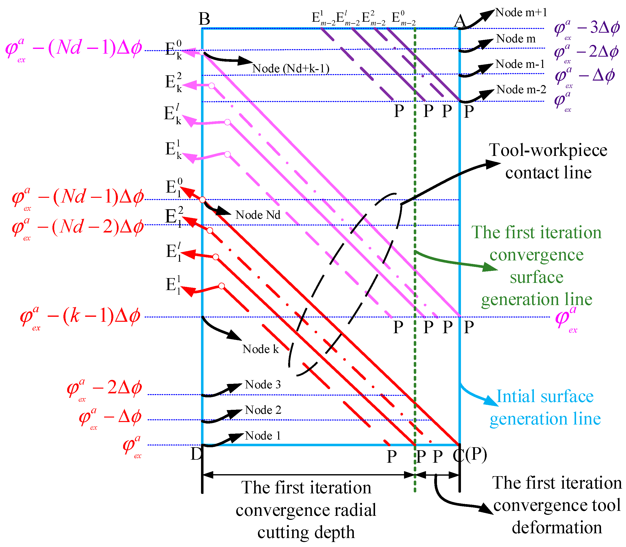
The initial entry angle and the number of nodes in contact are calculated. If the tool–workpiece contact is as in Case 1, the number of contact nodes along the axis is calculated using Equation (24). If the tool–workpiece contact is as in Case 2, the number of contact nodes along the axis is calculated using Equation (30).

Step 3:

Equations (11) and (25) are used to calculate the engagement angle of each node, so that the contact force of each node can be obtained based on Equations (9)–(15).

Step 4:

According to the calculated node cutting force, the initial deformation of each node can be calculated by Equations (1)–(4). Furthermore, the deformation and entry angle of each iteration step are updated according to Equations (26)–(28).

Step 5:

According to Equation (29), whether the current iteration converges or not is judged. If the current iteration converges, the continuation of the current iteration is stopped. The tool rotates Δϕ to enter the next iteration, and steps 1 to 4 are repeated until all nodes are calculated.

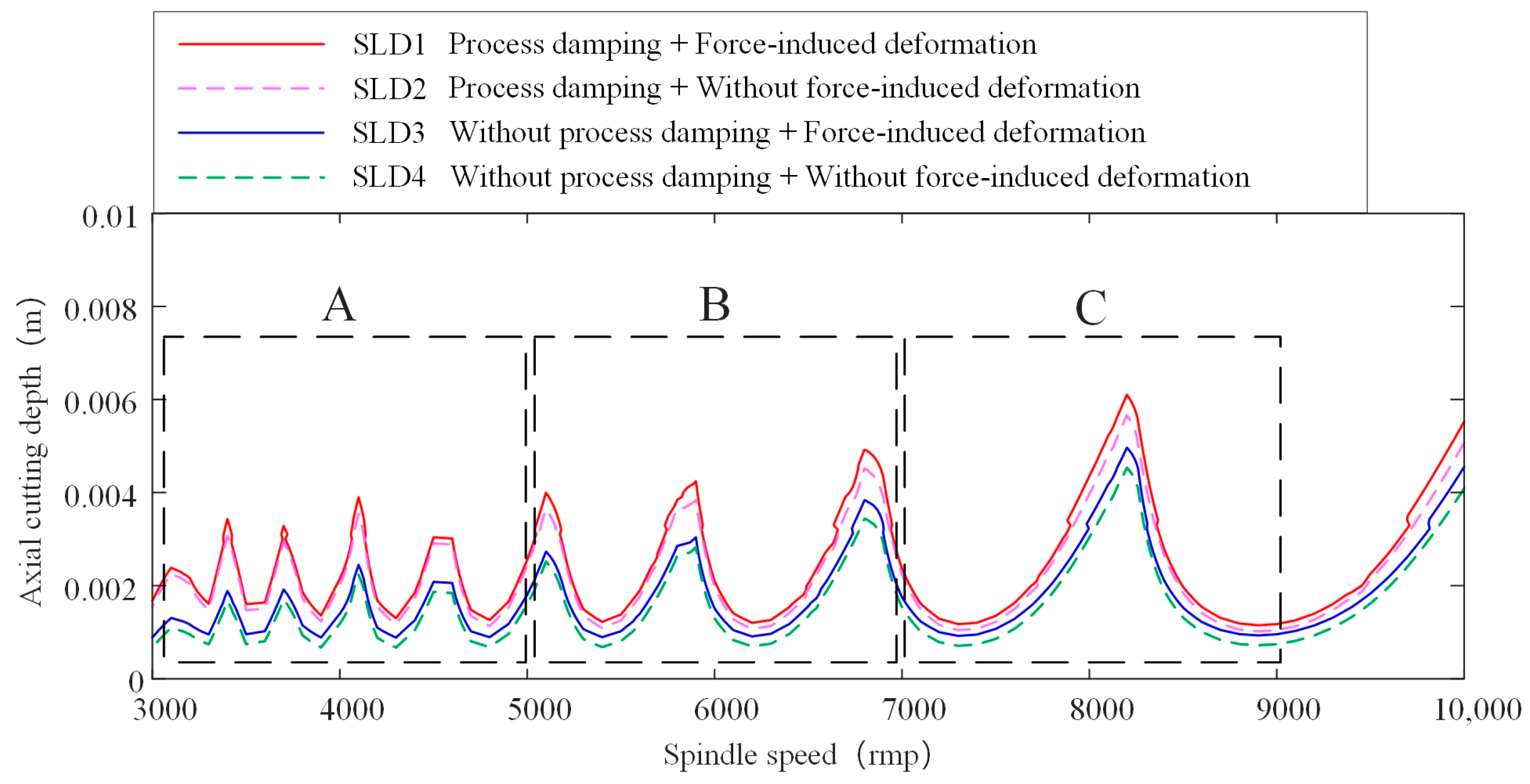
5. Solution of Stability Lobe Diagram

In order to take the multipoint contact dynamics and force-induced deformation effects into account simultaneously in the process of solving the stability lobe diagram (SLD), a full discrete method is presented based on the method proposed in [37]. By coordinate transformation, Equation (5) is converted from physical space to modal space as follows:

$${\mathit{M}}_q\ddot{\mathit{q}}(t)+{\mathit{C}}_q\dot{\mathit{q}}(t)+{\mathit{K}}_q\mathit{q}(t)={\mathbf{\psi }}^T\mathit{F}(t)$$

(32)

where $\mathit{q}\left(t\right)$ represents the displacement vector in the modal space, whose size is $2S\times 1$. ${\mathit{M}}_q$, ${\mathit{C}}_q$ and ${\mathit{K}}_q$ are the modal mass, damping and stiffness matrices of the robot milling system, respectively, which can be expressed as follows:

$${\mathit{M}}_q=\left[\mathit{I}\right]{\mathit{C}}_q=\left[2\mathbf{\xi }\mathbf{\omega }\right]{\mathit{K}}_q=\left[{\mathbf{\omega }}^2\right]$$

(33)

in which I is the diagonal identity matrix, $\mathbf{\xi }$ and $\mathbf{\omega }$ are damping ratio and natural frequency matrices, which are diagonal matrices with $2S\times 2S$ dimensions.

$$\xi ={\left[\begin{array}{ccccccc}{\xi }_{S,1}^x& & & & & & 0\\ & {\xi }_{S,1}^y& & & & & \\ & & {\xi }_{S,2}^x& & & & \\ & & & {\xi }_{S,2}^y& & & \\ & & & & \ddots & & \\ & & & & & {\xi }_{S,S}^x& \\ 0& & & & & & {\xi }_{S,S}^y\end{array}\right]}_{2S\times 2S}\omega ={\left[\begin{array}{ccccccc}{\omega }_{S,1}^x& & & & & & 0\\ & {\omega }_{S,1}^y& & & & & \\ & & {\omega }_{S,2}^x& & & & \\ & & & {\omega }_{S,2}^y& & & \\ & & & & \ddots & & \\ & & & & & {\omega }_{S,S}^x& \\ 0& & & & & & {\omega }_{S,S}^y\end{array}\right]}_{2S\times 2S}$$

(34)

in which S represents the number of dominant modes. $\mathbf{\psi }$ is the mass normalized mode shape matrix in the dominant mode with size $2\left(m+1\right)\times 2S$, which can be expressed as Equation (35):

$$\psi ={\left[\begin{array}{ccccccc}{\psi }_{S,1,1}^{x,x}& {\psi }_{S,1,1}^{y,x}& {\psi }_{S,2,1}^{x,x}& {\psi }_{S,2,1}^{y,x}& \cdots & {\psi }_{S,S,1}^{x,x}& {\psi }_{S,S,1}^{y,x}\\ {\psi }_{S,1,1}^{x,y}& {\psi }_{S,1,1}^{y,y}& {\psi }_{S,2,1}^{x,y}& {\psi }_{S,2,1}^{y,y}& \cdots & {\psi }_{S,S,1}^{x,y}& {\psi }_{S,S,1}^{y,y}\\ {\psi }_{S,1,2}^{x,x}& {\psi }_{S,1,2}^{y,x}& {\psi }_{S,2,2}^{x,x}& {\psi }_{S,2,2}^{y,x}& \cdots & {\psi }_{S,S,2}^{x,x}& {\psi }_{S,S,2}^{y,x}\\ {\psi }_{S,1,2}^{x,y}& {\psi }_{S,1,2}^{y,y}& {\psi }_{S,2,2}^{x,y}& {\psi }_{S,2,2}^{y,y}& \cdots & {\psi }_{S,S,2}^{x,y}& {\psi }_{S,S,2}^{y,y}\\ ⋮& ⋮& ⋮& ⋮& \cdots & ⋮& ⋮\\ {\psi }_{S,1,m+1}^{x,x}& {\psi }_{S,1,m+1}^{y,x}& {\psi }_{S,2,m+1}^{x,x}& {\psi }_{S,2,m+1}^{y,x}& \cdots & {\psi }_{S,S,m+1}^{x,x}& {\psi }_{S,S,m+1}^{y,x}\\ {\psi }_{S,1,m+1}^{x,y}& {\psi }_{S,1,m+1}^{y,y}& {\psi }_{S,2,m+1}^{x,y}& {\psi }_{S,2,m+1}^{y,y}& \cdots & {\psi }_{S,S,m+1}^{x,y}& {\psi }_{S,S,m+1}^{y,y}\end{array}\right]}_{2(m+1)\times 2S}$$

(35)

where ${\psi }_{S,u,k}^{o,p}$ represents the mode shape displacement of the k axial node in the p direction under the dominant mode of the u order when the main vibration is in the o direction. When o and p are in different directions, it represents the structural modal coupling effect of the tool due to the helical flute structure. It is worth noting that when the coupling effect of tool structure modes is not considered, the mode displacement of the cross modes in the matrix is considered to be 0.

The expression of cutting force in Equation (32) is shown as follows:

$$\mathit{F}(t)={\mathit{F}}^{\mathrm{s}}(t)+{\mathit{C}}_{\mathrm{p}}(t)\dot{\mathit{q}}(t)+\mathit{H}(t)[\mathit{q}(t)-\mathit{q}(t-T)]$$

(36)

where the static forces ${\mathit{F}}^{\mathrm{s}}\left(t\right)$ can be neglected in the calculation of stability [31]. $\mathit{H}\left(t\right)$ and ${\mathit{C}}_{\mathrm{p}}\left(t\right)$ represent the coefficient matrix of the regeneration term and process damping term, which can be expressed as follows:

$$\mathit{H}(t)=\left[\begin{array}{ccccc}{h}_{xx,1}& h_{xy,1}& & & \\ h_{yx,1}& h_{yy,1}& & & \\ & & \ddots & & \\ & & & h_{xx,m+1}& h_{xy,m+1}\\ & & & h_{yx,m+1}& h_{yy,m+1}\end{array}\right]\mathbf{\psi }\mathrm{and}\{\begin{array}{l}{h}_{xx,k}={\displaystyle \sum _{j=1}^N{g}_{j,k}^a(K_{tc}SC-K_{rc}{C}^2)dz}\hfill \\ h_{xy,k}={\displaystyle \sum _{j=1}^N{g}_{j,k}^a(-K_{tc}{S}^2+K_{rc}SC)dz}\hfill \\ h_{yx,k}={\displaystyle \sum _{j=1}^N{g}_{j,k}^a(K_{tc}{C}^2+K_{rc}SC)dz}\hfill \\ h_{yy,k}={\displaystyle \sum _{j=1}^N{g}_{j,k}^a(-K_{tc}SC-K_{rc}{S}^2)dz}\hfill \end{array}$$

(37)

$${\mathit{C}}_p(t)=\left[\begin{array}{ccccc}{c}_{p,xx,1}& c_{p,xy,1}& & & \\ c_{p,yx,1}& c_{p,yy,1}& & & \\ & & \ddots & & \\ & & & c_{p,xx,m+1}& c_{p,xy,m+1}\\ & & & c_{p,yx,m+1}& c_{p,yy,m+1}\end{array}\right]\mathbf{\psi }\mathrm{and}\{\begin{array}{c}{c}_{p,xx,k}={\displaystyle \sum _{j=1}^N{C}_{eq}{g}_{j,k}^a(\mu SC-C^2)}\\ c_{p,xy,k}={\displaystyle \sum _{j=1}^N{C}_{eq}{g}_{j,k}^a(-\mu S^2+SC)}\\ c_{p,yx,k}={\displaystyle \sum _{j=1}^N{C}_{eq}{g}_{j,k}^a(\mu C^2+SC)}\\ c_{p,yy,k}={\displaystyle \sum _{j=1}^N{C}_{eq}{g}_{j,k}^a(-\mu SC-S^2)}\end{array}$$

(38)

Using the method proposed in [25], the state transition matrix of the robot milling system over a tooth pass period T can be obtained, and the stability of the robot milling can be determined according to the Floquet theory [40,41].

6. Experimental Verification

In order to verify the chatter stability prediction effect of the above method, milling experiments were carried out on a KUKA KR600 robot. The verification experiments mainly consisted of four steps: robot joint stiffness identification, milling force coefficients identification, dynamic parameters identification and robot milling experiment verification. The first two steps were used to calculate the force-induced deformation of the robot milling system; the second and third steps were used to provide the required parameters for the SLD solution. Robot milling experiments were performed to verify the accuracy of the predicted SLD. The details of each step are elaborated as follows.

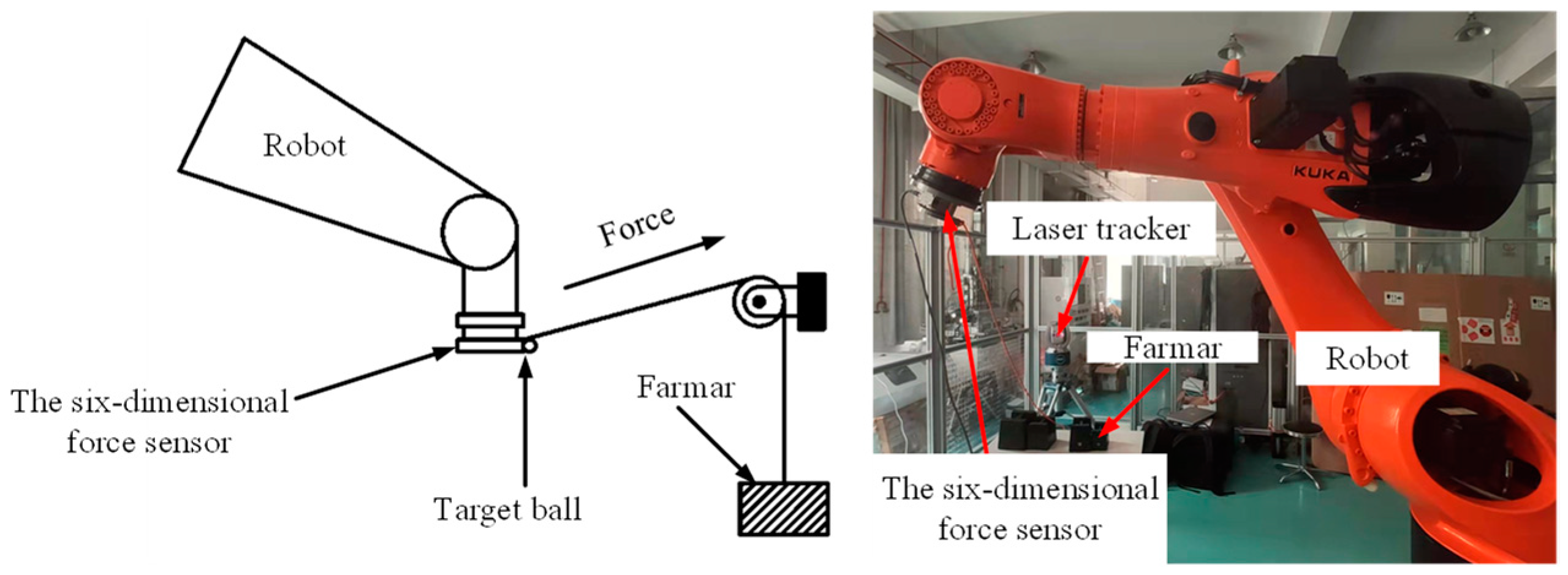
6.1. Robot Joint Stiffness Identification

Through the calculation principle of joint stiffness proposed in [42], the joint stiffness of the robot was calculated by measuring the displacement generated by corresponding external force at the end of the robot. Specifically, a load was applied at a certain point on the robot flange, the displacement deviation between the loaded state and the no-load state was compared, and the load mass and the force application direction were changed several times. Finally, the least squares method was used to fit the stiffness value of each joint of the robot.

According to the above steps, the laser tracker (API Co., Ltd., Rockwell City, IA, USA) was used to measure displacement deviation under load and no-load conditions. The six-dimensional force sensor (ATI Co., Ltd., Taipei, Taiwan) was used to measure the magnitude and direction of the applied external force. The experimental principle and test process are shown in Figure 8. During the experiments, we selected eight groups of different robot postures, respectively, measured the coordinates of the end target ball under no-load, 30 kg load and 50 kg load, respectively, calculated the displacement variable before and after loading, and used the six-dimensional force sensor to measure the corresponding external force. We repeated the measurement twice at each selected posture, and recorded the coordinates of the force point at the end of the robot and the measurement point in the base coordinate system to calculate the Jacobian matrix of the two points. Finally, the joint stiffness could be calculated as:

$${\mathit{K}}_{\mathrm{q}}=\mathrm{diag}[6.082\times {10}^6,6.816\times {10}^6,3.842\times {10}^6,2.926\times {10}^6,1.635\times {10}^6,2.479\times {10}^6] \mathrm{N}·\mathrm{m}/\mathrm{rad}$$

6.2. Milling Force Coefficient Identification

The milling force coefficient identification experiments were carried out on 5A06 aluminum alloy, adopting the slot milling method with variable process parameters as shown in Figure 9. A 3-tooth cemented carbide end mill with 45° helix angle was used, and the milling force was measured by a dynamometer (KISTLER 9257B) during the milling experiments. By averaging the cutting forces in the x and y directions under different milling parameters, the milling force coefficients were finally calculated as follows:

$$\{\begin{array}{c}{K}_{\mathrm{tc}}=855.00 \mathrm{N}/{\mathrm{mm}}^2\\ K_{\mathrm{rc}}=270.93 \mathrm{N}/{\mathrm{mm}}^2\\ K_{\mathrm{t}\mathrm{e}}=15.64 \mathrm{N}/\mathrm{mm}\\ K_{\mathrm{re}}=14.167 \mathrm{N}/\mathrm{mm}\end{array}$$

(39)

6.3. Tool Dynamic Parameters Identification

The dynamic parameters of the tool in the robot milling system were identified by the EMA hammer test. A hammer equipped with a YD-5T quartz sensor was selected to obtain the excitation signal, and an eddy current sensor was used to obtain the vibration response signal. During the hammer test, the overhang length of the tool was 61 mm, and the poses of the robot were selected to be consistent with the machining process, which were −71.73°, −68.62°, 110.51°, 35.54°, −47.68°, −204.68°, as shown in Figure 10. Considering the degrees of freedom of the robot milling dynamics model, four points with different distances from the free end of the tool were selected for the hammer test in feed (x) and normal (y) directions, which were defined as follows: (1) in feed direction, P1_x, P2_x, P3_x and P4_x were located at 3, 12, 24, 36 mm away from the free end of the tool; (2) in radial direction, P1_y, P2_y, P3_y and P4_y were located at 3, 12, 24, 36 mm away from the free end of the tool, as shown in Figure 10. The eddy current sensor was always installed at P1_x and P1_y positions; the modal parameters are identified and given in

Table 2. Dynamic parameter identification results.

Direction	Natural Frequency (Hz)	Damping Ratio (%)	Normalized Mode Shapes ( $1/\sqrt{\mathbf{kg}}$)
x	2060.49	2.37	P1x: 3.232 P2x: 2.264 P3x: 1.738 P4x: 1.075
y	2045.24	2.07	P1y: 4.119 P2y: 3.347 P3y: 2.315 P4y: 1.755

.

6.4. Milling Experiment Verification

The force-induced deformation of a robot milling system can be obtained by numerical simulation based on the parameters identified by the above experiments. Taking the deformation of node (k = 1) at the free end of the tool as an example, the variation law of deformation with axial cutting depth is shown in Figure 11a. It can be seen that the deformation of node 1 gradually increases with the increase of axial cutting depth, because the cutting force increases with the increase of axial cutting depth. Figure 11b shows the change law of entry angle of node 1 with axial cutting depth. It increases with the increase of axial cutting depth. It is worth noting that when the axial cutting depth reaches the limit value of Equation (22), the deformation of node 1 will no longer increase. This is because when the axial cutting depth exceeds the critical value, the tool–workpiece contact state changes to that in Case (2), and the number of tool–workpiece contact nodes no longer increases; as shown in Figure 6, the length of $E_1^{0}P$ does not change as BD increase.

When the radial cutting depth is 4 mm and the feed speed is 600 mm/min, SLDs considering different factors are predicted as shown in Figure 12. Some sets of milling tests at different speeds are selected in regions A, B and C in the figure to verify the accuracy of the SLDs, as shown in Figure 13. The stability limit of a certain speed is determined by the milling method with increasing axial cutting depth, as shown in Figure 14a. Acceleration sensor is used to determine whether chatter occurs during milling. The experiment process is shown in Figure 14b.

In Figure 13, SLD1 and SLD2 are the prediction results of chatter stability before and after considering force-induced deformation, which simultaneously consider regeneration effect and process damping. Obvious deviation can be found between the two SLDs, especially at the crest of the SLD. According to the prediction results, the region between the two SLDs is predicted as a chatter region by SLD2, but according to the experimental results, this region is judged to be the stable region, and the result is consistent with the prediction result of SLD1. This indicates that considering force-induced deformation will make the prediction of SLD more accurate. The comparison results of SLD3 and SLD4 also prove the above conclusion. In addition, SLD1 and SLD4 are the prediction results of chatter stability before and after considering process damping and force-induced deformation. As can be seen from Figure 13, more significant deviation is observed when process damping is taken into account. The experimental results show that the prediction result of SLD can be greatly improved when both process damping and force-induced deformation are considered. In order not to lose generality, three groups of acceleration signals at different spindle speeds (3600 rpm, 7200 rpm and 8000 rpm) were analyzed. The acceleration signals are illustrated in Figure 15, Figure 16 and Figure 17, and the frequency spectrum generated by fast Fourier transformation (FFT) of the acceleration signals are given in the same figure. It can be clearly seen in the spectrum that when the processing is in the stable stage, all the components of the spectrum are spindle frequency, tooth passing frequencies and their harmonics. When the processing is in the chatter stage, the chatter frequencies are observed on the spectrum, which are different from spindle frequency, tooth passing frequencies and their harmonics.

In conclusion, compared with the traditional model, the predicted stability region after considering the milling deformation will be expanded. The predicted expanded stability region was verified as the stability region by robot milling experiments. This shows that compared with the traditional model, the established dynamic model considering milling deformation can predict the robot milling stability more accurately. This is due to the fact that traditional models have ignored the factor of deformation in robot milling and considered the tool workpiece contact area as constant during milling process. However, through the deformation analysis of the robot milling system, it can be seen that the milling deformation will cause the dynamic change of the tool–workpiece contact area and the increase of the cutting angle boundary, which has a direct influence on the milling stability prediction. Therefore, the milling deformation is considered in the robot milling dynamics model in this paper, which can reflect the actual machining process more accurately, and a more accurate prediction results can be obtained.

7. Conclusions

This paper focuses on the influence of deformation on chatter stability during robot milling. A dynamic model of robot milling considering milling deformation is established and the SLD is predicted based on the model. The results are as follows:

(1) The influence mechanism of milling deformation on robot milling stability is analyzed. The results show that the milling deformation will reduce the tool–workpiece contact area and increase the cutting angle boundary, which will affect the milling stability.

(2) An iterative calculation strategy for milling deformation is proposed. This strategy takes into account the different contact states between tool and workpiece, which realizes the calculation of milling deformation under different process parameters. The results show that the milling deformation varies with the spindle speed and the axial cutting depth. When the spindle speed is 10,000 rpm, the maximum deformation can exceed 0.09 mm, causing the cutting angle boundary to increase by more than 1°.

(3) A multipoint contact dynamic model of robot milling is established, which considers the influence of milling deformation on regenerative effect and process damping. A fully discrete method is applied to predict the SLD of robot milling and the stability prediction results show that compared with the traditional model, the predicted stability area is further expanded by considering milling deformation and process damping. The predicted expanded stability region is verified as the stability region by robot milling experiments. These show that compared with the traditional model, the established dynamic model considering milling deformation can predict the robot milling stability more accurately.

References

1. Liao, Z.; Li, J.; Xie, H.; Wang, Q.; Zhou, X. Region-based tool path generation for robot milling of freeform surfaces with stiffness optimization. Robot. Comput. Integr. Manuf. 2020, 64, 101953. [Google Scholar] [CrossRef]
2. Zhu, D.; Feng, X.; Xu, X.; Yang, Z.; Ding, H. Robot grinding of complex components: A step towards efficient and intelligent machining—Challenges, solutions, and applications. Robot. Comput. Integr. Manuf. 2020, 65, 101908. [Google Scholar] [CrossRef]
3. Zhu, Z.; Tang, X.; Chen, C.; Peng, F.; Wu, J. High precision and efficiency robot milling of complex parts: Challenges, approaches and trends. Chin. J. Aeronaut. 2022, 35, 22–46. [Google Scholar] [CrossRef]
4. Chen, Q.; Zhang, C.; Hu, T.; Zhou, Y.; Ni, H.; Xue, X. Posture optimization in robotic machining based on comprehensive deformation index considering spindle weight and cutting force. Robot. Comput. Integr. Manuf. 2021, 74, 102290. [Google Scholar] [CrossRef]
5. Lin, J.; Ye, C.; Yang, J.; Zhao, H.; Ding, H.; Luo, M. Contour error-based optimization of the end-effector pose of a 6 degree-of-freedom serial robot in milling operation. Robot. Comput. Integr. Manuf. 2021, 73, 102257. [Google Scholar] [CrossRef]
6. Huynh, H.; Assadi, H.; Dambly, V.; Rivière-Lorphèvre, E.; Verlinden, O. Direct method for updating flexible multibody systems applied to a milling robot. Robot. Comput. Integr. Manuf. 2020, 68, 102049. [Google Scholar] [CrossRef]
7. Maamar, L. Pose-dependent modal behavior of a milling robot in service. Int. J. Adv. Manuf. Technol. 2020, 107, 527–533. [Google Scholar] [CrossRef]
8. Yuan, L.; Pan, Z.; Ding, D.; Sun, S.; Li, W. A Review on Chatter in Robotic Machining Process Regarding Both Regenerative and Mode Coupling Mechanism. IEEE/ASME Trans. Mechatron. 2018, 23, 2240–2251. [Google Scholar] [CrossRef]
9. Tunc, T.; Gonul, B. Effect of quasi-static motion on the dynamics and stability of robotic milling. CIRP Ann. 2021, 70, 305–308. [Google Scholar] [CrossRef]
10. Nguyen, V.; Johnson, J.; Melkote, S. Active vibration suppression in robotic milling using optimal control. Int. J. Mach. Tools Manuf. 2020, 152, 103541. [Google Scholar] [CrossRef]
11. Faassen, R.P.H.; van de Wouw, N.; Oosterling, J.A.J.; Nijmeijer, H. Prediction of regenerative chatter by modelling and analysis of high-speed milling. Int. J. Mach. Tools. Manuf. 2003, 43, 1437–1446. [Google Scholar] [CrossRef]
12. Zhu, L.; Liu, C. Recent progress of chatter prediction, detection and suppression in milling. Mech. Syst. Signal Process. 2020, 143, 106840. [Google Scholar] [CrossRef]
13. Altintaş, Y.; Budak, E. Analytical Prediction of Stability Lobes in Milling. CIRP Ann. 1995, 44, 357–362. [Google Scholar] [CrossRef]
14. Budak, E. Mechanics and Dynamics of Milling Thin Walled Structures; University of British Columbia: Vancouver, BC, Canada, 1994. [Google Scholar]
15. Eksioglu, C.; Kilic, Z.M.; Altintas, Y. Discrete-Time Prediction of Chatter Stability, Cutting Forces, and Surface Location Errors in Flexible Milling Systems. J. Manuf. Sci. Eng. 2012, 134, 061006. [Google Scholar] [CrossRef]
16. Merdol, S.D.; Altintas, Y. Multi Frequency Solution of Chatter Stability for Low Immersion Milling. J. Manuf. Sci. Eng. 2004, 126, 459–466. [Google Scholar] [CrossRef]
17. Budak, E.; Altintas¸, Y. Analytical Prediction of Chatter Stability in Milling—Part I: General Formulation. J. Dyn. Syst. Meas. Control 1998, 120, 22–30. [Google Scholar] [CrossRef]
18. Insperger, T.; Stépán, G. Updated semi-discretization method for periodic delay-differential equations with discrete delay. Int. J. Numer. Methods Eng. 2004, 61, 117–141. [Google Scholar] [CrossRef]
19. Insperger, T. Full-discretization and semi-discretization for milling stability prediction: Some comments. Int. J. Mach. Tools Manuf. 2010, 50, 658–662. [Google Scholar] [CrossRef]
20. Ding, Y.; Zhu, L.; Zhang, X.; Ding, H. A full-discretization method for prediction of milling stability. Int. J. Mach. Tools Manuf. 2010, 50, 502–509. [Google Scholar] [CrossRef]
21. Mousavi, S.; Gagnol, V.; Bouzgarrou, B.C.; Ray, P. Stability optimization in robotic milling through the control of functional redundancies. Robot. Comput. Integr. Manuf. 2018, 50, 181–192. [Google Scholar] [CrossRef]
22. Mousavi, S.; Gagnol, V.; Bouzgarrou, B.C.; Ray, P. Control of a Multi Degrees Functional Redundancies Robotic Cell for Optimization of the Machining Stability. Procedia CIRP 2017, 58, 269–274. [Google Scholar] [CrossRef]
23. Gonul, B.; Sapmaz, O.F.; Tunc, L.T. Improved stable conditions in robotic milling by kinematic redundancy. Procedia CIRP 2019, 82, 485–490. [Google Scholar] [CrossRef]
24. Cordes, M.; Hintze, W.; Altintas, Y. Chatter stability in robotic milling. Robot. Comput. Integr. Manuf. 2019, 55, 11–18. [Google Scholar] [CrossRef]
25. Mejri, S.; Gagnol, V.; Le, T.-P.; Sabourin, L.; Ray, P.; Paultre, P. Dynamic characterization of machining robot and stability analysis. Int. J. Adv. Manuf. Technol. 2016, 82, 351–359. [Google Scholar] [CrossRef]
26. Quintana, G.; Ciurana, J. Chatter in machining processes: A review. Int. J. Mach. Tools Manuf. 2011, 51, 363–376. [Google Scholar] [CrossRef]
27. Xin, S.; Peng, F.; Tang, X.; Yan, R.; Li, Z.; Wu, J. Research on the influence of robot structural mode on regenerative chatter in milling and analysis of stability boundary improvement domain. Int. J. Mach. Tools Manuf. 2022, 179, 103918. [Google Scholar] [CrossRef]
28. Li, J.; Li, B.; Shen, N.; Qian, H.; Guo, Z. Effect of the cutter path and the workpiece clamping position on the stability of the robotic milling system. Int. J. Adv. Manuf. Technol. 2017, 89, 2919–2933. [Google Scholar] [CrossRef]
29. Mohammadi, Y.; Ahmadi, K. Effect of axial vibrations on regenerative chatter in robotic milling. Procedia CIRP 2019, 82, 503–508. [Google Scholar] [CrossRef]
30. Wang, R.; Li, F.; Niu, J.; Sun, Y. Prediction of pose-dependent modal properties and stability limits in robotic ball-end milling. Robot. Comput. Integr. Manuf. 2022, 75, 102307. [Google Scholar] [CrossRef]
31. Sun, Y.; Jiang, S. Predictive modeling of chatter stability considering force-induced deformation effect in milling thin-walled parts. Int. J. Mach. Tools Manuf. 2018, 135, 38–52. [Google Scholar] [CrossRef]
32. Kang, Y.-G.; Wang, Z.-Q. Two efficient iterative algorithms for error prediction in peripheral milling of thin-walled workpieces considering the in-cutting chip. Int. J. Mach. Tools Manuf. 2013, 73, 55–61. [Google Scholar] [CrossRef]
33. Wan, M.; Zhang, W.; Qin, G.; Wang, Z.-P. Strategies for error prediction and error control in peripheral milling of thin-walled workpiece. Int. J. Mach. Tools Manuf. 2008, 48, 1366–1374. [Google Scholar] [CrossRef]
34. Li, Z.-L.; Tuysuz, O.; Zhu, L.-M.; Altintas, Y. Surface form error prediction in five-axis flank milling of thin-walled parts. Int. J. Mach. Tools Manuf. 2018, 128, 21–32. [Google Scholar] [CrossRef]
35. Whitney, D.E. The Mathematics of Coordinated Control of Prosthetic Arms and Manipulators. J. Dyn. Syst. Meas. Control 1972, 94, 303–309. [Google Scholar] [CrossRef]
36. Ahmadi, K.; Ismail, F. Stability lobes in milling including process damping and utilizing Multi-Frequency and Semi-Discretization Methods. Int. J. Mach. Tools Manuf. 2012, 54–55, 46–54. [Google Scholar] [CrossRef]
37. Ji, Y.; Wang, X.; Liu, Z.; Wang, H.; Jiao, L.; Zhang, L.; Tao, H. Milling stability prediction with simultaneously considering the multiplefactors coupling effects—Regenerative effect, mode coupling, and process damping. Int. J. Adv. Manuf. Technol. 2018, 97, 2509–2527. [Google Scholar] [CrossRef]
38. Budak, E.; Altintas, Y. Peripheral milling conditions for improved dimensional accuracy. Int. J. Mach. Tools Manuf. 1994, 34, 907–918. [Google Scholar] [CrossRef]
39. Wan, M.; Zhang, W.; Qiu, K.; Gao, T.; Yang, Y. Numerical Prediction of Static Form Errors in Peripheral Milling of Thin-Walled Workpieces with Irregular Meshes. J. Manuf. Sci. Eng. 2005, 127, 13–22. [Google Scholar] [CrossRef]
40. Lakshmikantham, V.; Trigiante, D. Theory of Difference Equations, Numerical Methods and Applications; Academic Press: London, UK, 1988. [Google Scholar]
41. Kolmanovskii, V.B.; Nosov, V.R. Stability of Functional Differential Equations; Academic Press: London, UK, 1986. [Google Scholar]
42. Liang, Z.; Shi, G.; Du, Y.; Ye, Y.; Ji, Y.; Chen, S.; Qiu, T.; Liu, Z.; Zhou, T.; Wang, X. Research on Tooltip Frequency Response Prediction of Robot Milling System Considering the Characteristics of spindle-toolholder interface. China Mech. Eng. 2022, 34, 2. [Google Scholar]
Figure 1. The deformation principle in the process of the robot milling. (a) Tool deformation; (b) Robot deformation.
Metals 13 00974 g001
Figure 2. Two degrees of freedom milling dynamics model.
Metals 13 00974 g002
Figure 3. The effect of force-induced deformation on milling process. (a) Change in entry angle due to deformation; (b) Change in cutting thickness due to deformation.
Metals 13 00974 g003
Figure 4. The tool–workpiece contact state.
Metals 13 00974 g004
Figure 5. Deformation iterative calculation process in Case 1.
Metals 13 00974 g005
Figure 6. Deformation iterative calculation process in Case 2.
Metals 13 00974 g006
Figure 7. Deformation calculation algorithm logic diagram.
Metals 13 00974 g007
Figure 8. Principle and experiment of robot joint stiffness identification.
Metals 13 00974 g008
Figure 9. The milling force identification experiment.
Metals 13 00974 g009
Figure 10. Tool dynamic parameters identification.
Metals 13 00974 g010
Figure 11. The variation law of deformation with axial cutting depth (the spindle speed is 10,000 r/min, radial cutting depth is 4 mm and the feed speed is 600 mm/min). (a) Radial cutting depth variation; (b) Entry angle variation.
Metals 13 00974 g011
Figure 12. SLD considering different factors.
Metals 13 00974 g012
Figure 13. Experimental verification results.
Metals 13 00974 g013
Figure 14. Milling test (a): milling with variable cutting depth (b): robot milling process.
Metals 13 00974 g014
Figure 15. Acceleration signal at 3600 r/min: (a) original signal; (b) stable signal frequency spectrum; (c) chatter signal frequency spectrum.
Metals 13 00974 g015
Figure 16. Acceleration signal at 7200 r/min: (a) original signal; (b) stable signal frequency spectrum; (c) chatter signal frequency spectrum.
Metals 13 00974 g016
Figure 17. Acceleration signal at 8000 r/min: (a) original signal; (b) stable signal frequency spectrum; (c) chatter signal frequency spectrum.
Metals 13 00974 g017