Influencing Factors of the Specific Total Loss of Non-Oriented Electrical Steels Processed by Laser Cutting

Abstract

Specific total loss is one of the most important evaluation indexes for the magnetic properties of non-oriented electrical steel sheets. The aim of this study is to investigate the influencing mechanisms of laser cutting parameters as well as the sample characteristics on the specific total loss of thin non-oriented electrical steel sheets processed by laser cutting using a machine learning method. Eight input parameters were finally considered; namely, silicon and manganese contents, thickness of the steel sheets, laser nozzle diameter, laser power, cutting speed, the pressure of process gas, and laser defocus, while one output parameter, the specific total loss, was evaluated. It was found that the specific total loss was positively correlated with the sample thickness, but negatively correlated with silicon and manganese contents, the process gas pressure and laser nozzle diameter. In addition, laser power and cutting speed exhibit complicated non-linear relationships with the specific total loss.

1. Introduction

Non-oriented electrical steel is an important soft magnetic material that is mainly utilized as core laminations for motors, transformers and generators. Low specific total loss and high magnetic induction intensify are typical of non-oriented electrical steels with excellent magnetic properties [1,2,3,4]. Specific total loss refers to the consumed electric energy per unit mass as the iron core manufactured with electrical steel is axially magnetized to a specific magnetic induction intensify at a certain frequency, which can be obtained from the magnetic measurements on the Epstein frame or by using the single sheet tester method. Specific total loss is also named as iron loss for short, with the unit W/kg. The non-oriented electrical steel is generally required to have low iron loss, which can not only save the electric energy, but also enhance the life of the motor and transformer [2]. At present, high-grade non-oriented electrical steel strips (sheets) are mainly manufactured by traditional machining methods such as mechanic shearing and punching. The plastic and elastic stresses as well as the shear deformation induced by mechanical shearing could result in the deterioration in magnetic properties of the electrical steels [5,6] and the efficiency of the core [7,8,9,10]. Meanwhile, laser cutting as an alternative to mechanic shearing has been gradually utilized in industry due to its ultra-flexibility of cutting conditions, high quality product, quick setup, non-mechanical contact between the workpiece and the tool, and the small size of the heat affected zone (HAZ) [11,12].

Nevertheless, some researchers have pointed out that laser cutting may further deteriorate the specific total loss of non-oriented electrical steel compared with traditional mechanic shearing [9,10]. To date, a lot of research has been carried out to investigate the effects of laser cutting parameters on the cut edge quality of electrical steel sheets [13,14,15,16,17,18,19,20,21]. It is generally accepted that the local microstructure, crystallographic texture, chemical composition, inclusion fraction as well as the stress state near the cut edge could be altered in the melting and solidification process induced by laser cutting [16,17,18]. The magnetic properties loss induced by mechanic shearing can be simply attributed to elastic and plastic deformation [22], whereas the quantitative study of the mechanisms influencing laser cutting parameters on the magnetic quality loss is difficult due to the large number of variables related to laser cutting (such as laser nozzle diameter, laser power, laser cutting speed, laser pulse frequency, laser defocus, process gas pressure, duty cycle, Kerf width, et cetera), the varying types of electrical steels (varying chemical composition and geometry) and the limited size of the heat affected zone near the cut edge [19,20,21]. In fact, for a new type of non-oriented electrical steel, many trial experiments need to be designed to determine the appropriate laser cutting parameter combination to guarantee the magnetic properties by taking the samples processed by traditional mechanic shearing as reference. Therefore, in industry, a simulation model to assist laser cutting parameter optimization is highly needed.

Because the mechanisms behind laser cutting are very complicated and process dependent [23,24], establishing the complicated non-linear relationship between laser cutting process parameters and the mechanic and magnetic properties has become a real challenging [25]. Recently, artificial intelligence methods have been utilized in the prediction of Kerf width [12,13,26,27,28], roughness quantification [29], and the size of the heat affected zone related to laser cutting [30]. Specifically, artificial neural network (ANN), random vector functional link network (RVFL), support vector regression (SVR), and Deep neural network (DNN) combined with genetic algorithm (GA) have been applied to predict laser cutting qualities based on laser process parameters [24,31,32,33]. However, to our knowledge, work related to the specific total loss analysis and prediction for non-oriented electrical steel processed by laser cutting using artificial intelligence methods has not been reported.

Although the combination abundance of the laser cutting parameters and the material characteristics result in time-consuming optimization procedures [34], the authors found that more attention should be given to laser power, the density and thickness of the steel sheet, laser cutting speed, laser defocus, process gas pressure, and laser nozzle diameter. In this work, the specific total loss index P_1.0/50 was utilized to the evaluate the magnetic properties of non-oriented electoral steel, and a popular machine learning method especially suitable to small datasets was chosen to train the model, correlating the laser cutting parameters to the specific total loss, with the aim to investigate the influencing mechanisms of material characteristics and laser cutting parameters on the magnetic properties of non-oriented electrical steel, and guide the design of laser cutting parameters.

2. Experiment

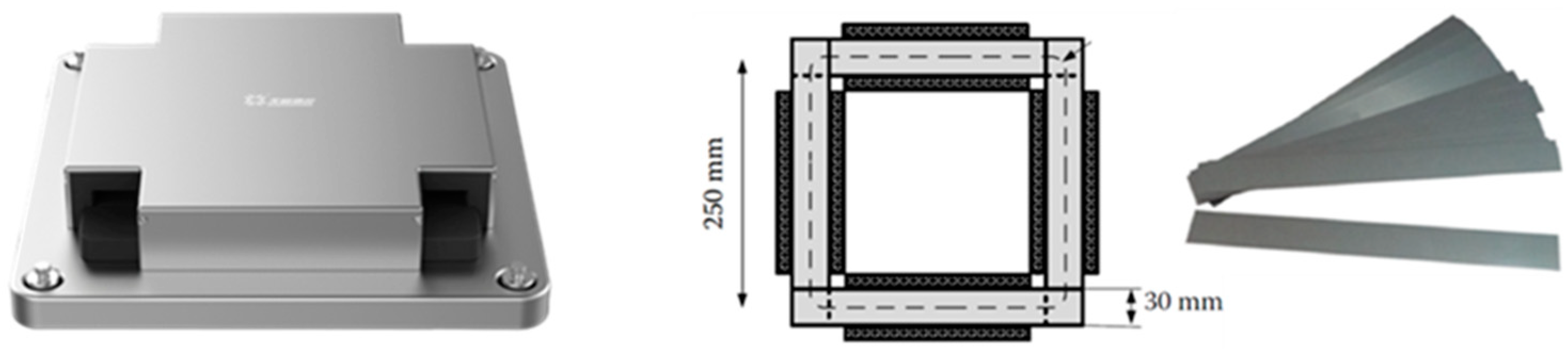
2.1. Experimental Methods and Data Collection

Six types of non-oriented electrical steel sheets were prepared in this work. The main chemical compositions as well as other physical quantities of these steels are shown in

Table 1. Nominal density, averaged chemical composition and resistivity.

No.	Density, g/cm3	w (Si), %	w (Al), %	w (Mn), %	Resistivity, μΩ·cm
1	7.60	3.328	0.971	0.218	64.19
2	7.65	2.582	0.493	0.481	49.35
3	7.70	1.815	0.353	0.282	38.87
4	7.75	1.556	0.321	0.599	35.54
5	7.80	1.114	0.135	0.410	28.07
6	7.85	0.617	0.059	0.232	21.48

. The nominal density of these steels was increased from 7.60 to 7.85 g/cm³ with an interval of 0.05 g/cm³, which was achieved by decreasing the Si and Al content. Specifically, Si content was decreased from 3.328 to 0.617 wt%, and correspondingly the Al content was decreased from 0.971 to 0.059 wt%, which was designed on purpose. Mass density decreased with the increasing Si content but the resistivity increased with increasing Si content, varying from 21.48 to 64.19 μΩ·cm. There was no obvious changing rule for Mn content. Before the featuring engineering, all five parameters were initially considered as the variables to train the machine learning model.

In this work, a pulsed YLR-2000 fiber laser emitting at 1.07 μm laser wavelength with a frequency of 5000 Hz was used in all the experiments. All these steel sheets with varying thickness were cut into the plate shape with the length of 320 mm and width of 30 mm. The compensation for the width loss induced by laser cutting kerf was set as 0.11 mm. The compensation for the width loss induced by laser cutting kerf was set as 0.11 mm. N₂ was chosen as the process gas, which was ejected from the nozzle and coaxial with the laser beam. Laser cutting height was set as 1 mm. The other varying parameters related to the laser cutting are laser nozzle diameter (‘nozzle diameter’, mm), cutting speed (m/min), laser power (W), process gas pressure (‘gas pressure’, MPa) and laser defocus (mm) as well as steel sheet thickness (‘thickness’, mm). These variables as well as the five material characteristics mentioned above were initially introduced in the machine learning model as the input. P_1.0/50 was chosen as the evaluation index of the magnetic properties. Here, P_1.0/50 represents the specific total loss measured at the frequency of 50 Hz with the maximum magnetic induction intensity of 1.0 T. The magnetic properties were measured using Epstein frame method (Figure 1) according to the national standard IEC 60404-2 “Magnetic materials-Part 2: Methods of measurement of the magnetic properties of electrical steel strip and sheet by means of an Epstein frame” [35]. 16 samples (8 pieces parallel and 8 pieces normal to the rolling direction) were needed for one round of magnetic properties measurement. 350 items were obtained in the original dataset by varying the type of steel and laser cutting parameter combinations. The magnetic domain structure was revealed by means of the Fe₃O₄ magnetic fluid method. Fe₃O₄ magnetic fluid was dripped on the interested surface of the prepared samples placed horizontally, and finally, after air drying, the optical observation was made on an optical metallographic microscope (ZEISS AX10). The cut edge was also directly observed using a scanning electron microscope (SEM, FEI Quanta FEG450).

2.2. Machine Leaning Algorithm

In the present work, an improved version of Gradient Boosting method [36,37], LightGBM, which demonstrates better training speed and prediction accuracy, was chosen as the machine learning algorithm. LightGBM is based on Gradient boosting and decision trees (GBDT) as well as XGBoost (eXtream gradient boosting). LightGBM yields better training speed and prediction accuracy by using improved measures such as histogram-based algorithms, which bucket the continuous values of features (attributes) into discrete bins, as shown in Figure 2a. Meanwhile, gradient-based one-side sampling (GOSS) is utilized in LightGBM for data sampling to deal with the problem of larger dataset, and exclusive feature bundling (EFB) is utilized for feature sampling to deal with the problem of larger numbers of features and to improve the efficiency of model training. Leaf-wise tree growth is implemented in LightGBM, wherein the leaf with maximum loss is selected to grow, and therefore the number of leaves at each level is not always the same, as shown in Figure 2b. Leaf-wise tree growth helps achieve a lower loss. In addition, the maximum depth (max-depth) of the tree can be set in the LightGBM model to limit the number of layers to control the complexity in the case of overfitting. It was reported that the learning time of LightGBM was 20 times shorter than that of the conventional GBDT algorithm with the same accuracy [36]. The performance of LightGBM has been proven in many studies [36,37,38,39,40,41] and in several famous data science competition platforms, such as Kaggle, Datacastle, and Data fountain.

2.3. Partial Dependence Plot (PDP)

In this work, PDP was utilized to explore the relationship between the features and specific total loss. The PDP plot shows the influence of the selected features (here, steel chemical composition, sample geometry, and laser cutting parameters) on the predicted results while marginalizing the other features. The partial dependence function for regression can be defined as

$${\stackrel{\wedge }{f}}_{xs}(x_S)=E_{xC}\left[\stackrel{}{\stackrel{\wedge }{f}\left[(x_S,x_C)\right]}\right]={\displaystyle \int \stackrel{}{\stackrel{\wedge }{f}(x_S,x_C)}}dP(x_C)$$

(1)

where x_S is the set of the features for which the partial dependence function should be plotted and x_C are the other features utilized in the machine learning model. Features x_S and the set x_C together make up the total feature space. By marginalizing over the features in set x_C, a function that depends on the features in x_S is obtained.

2.4. Statistical Evaluation Metrics (RMSE, MAE, EV, R²)

Four evaluation metrics are utilized in the present work, and the first one is Root-Mean-Square-Error (RMSE), which provides an absolute value for the average discrepancy between the predicted and experimental values. It is defined as

$$RMSE(y,\stackrel{\wedge }{y})=\sqrt{\frac{1}{n_{samples}}{\displaystyle \sum _{i=0}^{n_{samples}}{(y_i-\stackrel{\wedge }{y_i})}^2}}$$

(2)

Mean-Absolute-Error (MAE) is defined as

$$MAE(y,\stackrel{\wedge }{y})=\frac{1}{n_{samples}}{\displaystyle \sum _{i=0}^{n_{samples}}\left|y_i-\stackrel{\wedge }{y_i}\right|}$$

(3)

RMSE is more sensitive to outliers than MAE. The explained variation (EV) measures the proportion to which a statistical model accounts for the variation of a given dataset.

$$EV(y,\stackrel{\wedge }{y})=1-\frac{Var\{y-\stackrel{\wedge }{y}\}}{Var(y)}$$

(4)

The coefficient of determination (R²) is always a value between 0 and 1, and is estimated over the sampling size n_samples, where 1 represents a perfect agreement between the model and experiments. It is defined as

$$R^2(y,\stackrel{\wedge }{y})=1-\frac{{\displaystyle {\sum }_{i=0}^{n_{samples}-1}{(y_i-\stackrel{\wedge }{y_i})}^2}}{{\displaystyle {\sum }_{i=0}^{n_{samples}-1}{(y_i-{\overline{y}}_i)}^2}} \mathrm{and} \overline{y}=\frac{1}{n_{samples}}{\displaystyle \sum _0^{n_{samples}-1}{y}_i}\overline{y}=\frac{1}{n_{samples}}{\displaystyle \sum _0^{n_{samples}-1}{y}_i}$$

(5)

where $\stackrel{\wedge }{y_i}$ is the value of the i-th prediction, and y_i is the corresponding measured value.

3. Results and Discussion

3.1. Data Analysis

Figure 3 shows information on the dataset prepared for machine learning. It is clear that the distribution of values for each feature is not even. In the near future, this dataset could be enhanced. Items with small specific total loss outnumber the items with higher specific total loss. There is a clear gap between these two groups. Figure 4a demonstrates the correlation coefficients between the features. It is clear that steel density and resistivity exhibit strong correlation to Si content, i.e., 0.99 and 0.99, respectively. Meanwhile, Si also exhibits a strong correlation coefficient of 0.94 with Al, which is designed on purpose, as introduced above. Deleting the highly correlated features could speed up training and simplify the trained model, avoid over-fitting, and improve the generalization ability of the trained model. Therefore, in this work, Si remains the input feature because both density and resistivity of non-oriented electrical steels are highly dependent on Si content. Figure 4b demonstrates the correlation coefficients after feature engineering. It is clear that no strong correlation exists between any two of the remaining features. Finally, eight features (Si and Mn content, laser nozzle diameter, cutting speed, laser power, process gas pressure, laser defocus, and steel sheet thickness) were chosen as the input variables to train the machine learning model.

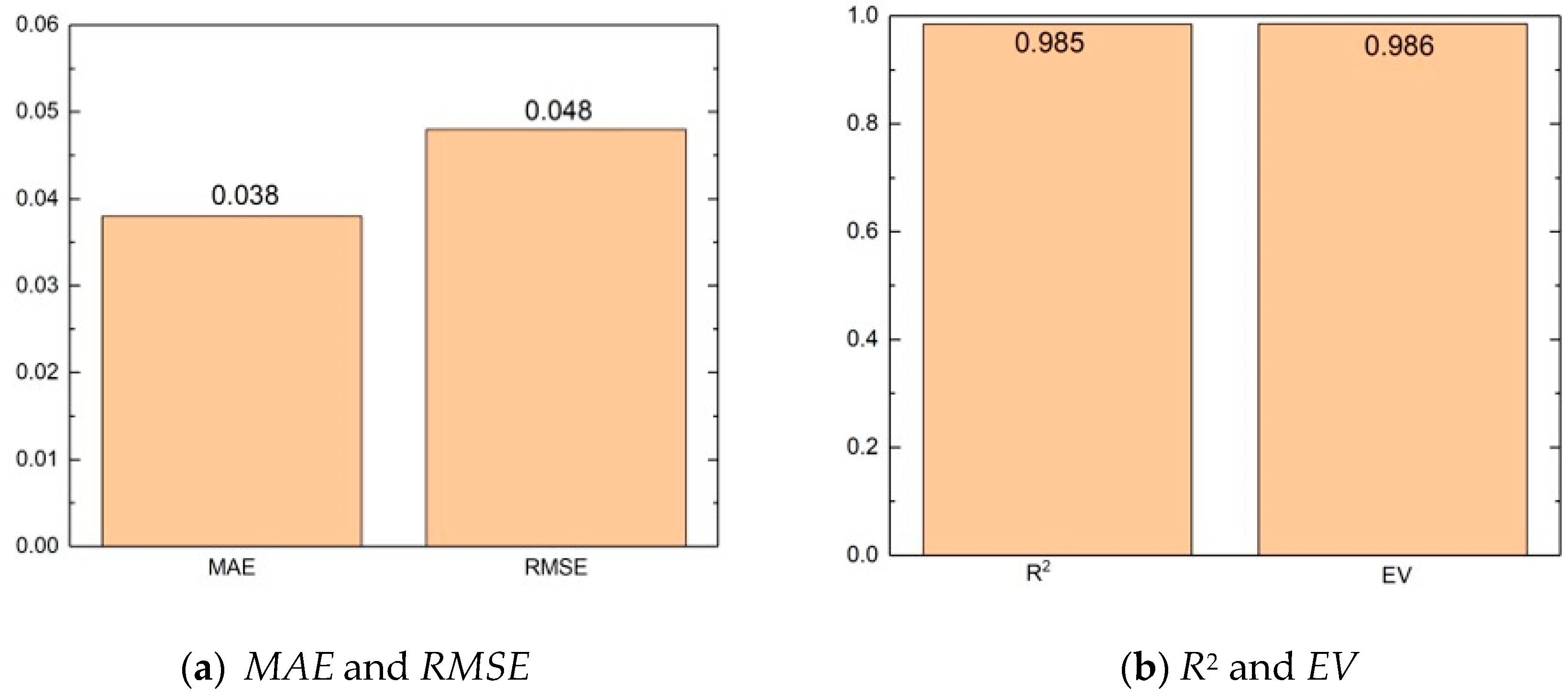
3.2. Performance of the Trained Model

Figure 5 shows the performance of the trained machine learning model. In this figure, the X-axis represents the experimental specific total loss and the Y-axis presents the predicted ones. It is clear that the correlation between the features and the specific total loss are fitted well by the LightGBM algorithm. Figure 6 further demonstrates that the fitted model exhibited low error and higher fitting score. The lower MAE and RMSE, the better the trained model. In this work, the MAE of 0.038 and RMSE of 0.048 are much smaller compared with the experimental specific total loss (varying in the range of 1.0 to 2.5 W/Kg), which indicates that the training error is small. Here, R² is a statistical measure of how close the data is to the fitted regression line. In general, for R², the closer to one, the better the model fits the dataset. For EV, the closer to one, the better the change in variance of the dependent variable can be explained by the independent variable. In this work, both R² (0.985) and EV (0.986) approach one, which indicates that the trained mode fits the dataset well. Figure 7 shows that laser power is considered the most important feature in the trained model, followed by the Si content, laser defocus, and cutting speed. Nozzle diameter is considered the least important feature, followed by the sample thickness and Mn content.

Figure 8c (PDP plot) demonstrates that only sample thickness is totally positively correlated with the specific total loss. Si and Mn content, laser nozzle diameter, Laser defocus, and process pressure are all negatively correlated with the specific total loss. Meanwhile, the specifical total loss could be significantly decreased with increasing Si content. Laser power and cutting speed exhibit a complicated non-linear relationship with the specific total loss, which indicates that it is difficult to predict the specific total loss by using a general fitting method. Specifically, the specific total loss firstly decreased with cutting speed and laser power, and then increased with further increases in cutting speed and laser power. However, the trained model can be utilized to predict the specifical total loss of the new given steel sheet to assist in optimizing the laser cutting parameters.

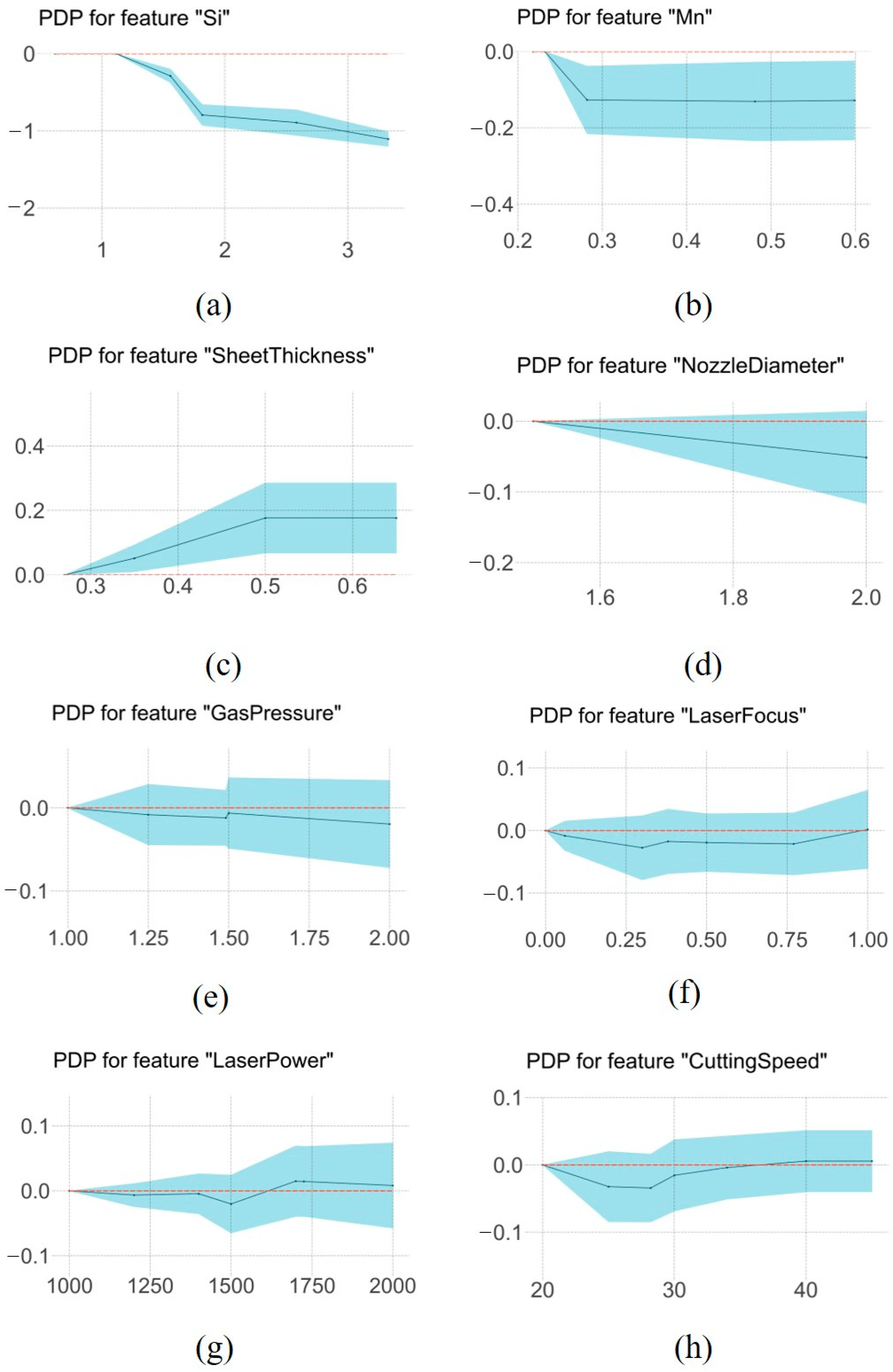
3.3. Effects of the Sample Characteristics on the Specific Total Loss

Generally speaking, the specific total loss of ferromagnetic materials is mainly composed of the hysteresis loss (P_h), eddy current loss (P_e), and residual loss (P_r). Based on the Bertotti model, the formula describing the dependence of energy loss on magnetic induction and frequency for non-oriented steel sheet takes the following form [42,43]

$$P_{tot}=P_h+P_c+P_{exc}=c_h{B}_m^{2}f+c_e{B}_m^2{f}^2+c_{exc}{B}_m^{1.5}{f}^{1.5}$$

(6)

$$c_h=2s/\mu \rho$$

(7)

$$c_e={\pi }^2\sigma d^2/6\rho$$

(8)

$$c_{exc}=8\sqrt{\sigma GS{V}_0}$$

(9)

$$s=\frac{\rho }{2B_{max}^2}\underset{f\to 0}{\lim }{\mu }_{f=0}\frac{P_{tot}}{f}$$

(10)

where P_tot is the total power loss per unit mass (W/Kg); B_m is the mean magnetic flux density throughout the sample (T); B_max is the maximum magnetic induction intensity (T); f is field frequency (Hz); c_h, c_e and c_exc are material-dependent coefficients; µ is magnetic permeability; s is defined as the quasi-static loop shape factor; ρ is mass density, σ is electrical conductivity; d is the sample thickness of the tested material cut as a strip; G is the damping parameter equal to 0.1356; S is the sheet cross-section area; and V₀ is the model parameter that characterizes the distribution of the internal coercive fields. The hysteresis loss (P_h) is proportional to the area of the static hysteresis loop of the investigated material, depending on the energy required for the magnetization. The residual loss is generally believed to be caused by the movement of the domain wall, which cannot be accurately quantified at present [44,45]. This will not be discussed in the present work due to its limited contribution to the specific total loss of non-oriented electrical steels.

In this work, the frequency of 50 Hz and the maximum magnetic induction intensity of 1.0 T (B_max) are fixed for all the tests. The eddy current loss is then proportional to the electrical conductivity and the square of the specimen thickness, and inversely proportional to the mass density [42,43]. As shown in Figure 8c, the specific total loss increased with the sample thickness. Meanwhile, as shown in Table 1, the electrical conductivity (the reciprocal of resistivity) gradually increased as the mass density increased from 7.60 to 7.85 g/cm³, which is consistent with Figure 8a. However, the dependence of eddy current loss on the mass density cannot be observed, since the specific total loss increased with the mass density, as shown in Figure 8a. In the one side, the change in amplitude of the resistivity is larger than that of mass density; in the other side, the hysteresis loss (P_h) contributes more to the specific total loss than the eddy current loss (P_e). Meanwhile, the mass density does not explicitly appear in the calculation of the final hysteresis loss because it vanishes by substituting s (Equation (10)) into c_h (Equation (7)). It is certain that the hysteresis loss (P_h) is inversely proportional to the magnetic permeability, which is dependent on the main chemical composition, crystal texture, inclusions, internal stress, grain size, sample thickness, and surface state, and can be significantly influenced by the laser cutting and mechanic shearing processes.

Silicon could decrease the AC core loss, hysteresis loss, classical eddy current loss, and apparent eddy current loss through the combined effects of grain coarsening, texture improvement, and increases in electrical resistivity [46]. Figure 9 shows the typical hysteresis curves at the maximum magnetic induction intensity of 1.0 T for the samples processed by laser cutting with the same processing parameters. It is clear that the hysteresis loss (P_h), i.e., the area of the hysteresis loop, decreased with the increasing Si content, which increased the resistivity and decreased the mass density. As Al varied in the range from 0.53 to 9.65 wt% in low silicon Fe-Al based non-oriented electrical steel, magnetic flux density and permeability tended to decrease as Al content increased, and in particular, as Al increased, P_h increased but P_e and P_exc decreased [43]. In this work, the effect of Al could be compromised by Si variance.

3.4. Effects of the Laser Cutting Parameters on the Specific Total Loss

In review of this modeling study on experimental investigations of CO₂ laser cutting quality, it is concluded that the main quality characteristics are the heat affected zone (HAZ) size, surface roughness, kerf width, and waviness of the cut edge as well as dross formation [47]. In this work, the main concern is the heat affected zone (HAZ) width and cut edge roughness induced by laser cutting, which could significantly influence the specific total loss. It is reported that the specific total loss can be significantly increased by the altered magnetic domain in HAZ induced by the laser cutting process as well as the residual stress [23]. Generally, an increase in cutting speed and a decrease in laser power result in a decrease in the width of the HAZ. However, it is also found that when using high laser power, the HAZ is extended with increasing cutting speed, which depends on both laser operation parameters and material properties [48].

In the literature, it was also reported that laser power, pulse frequency, and cutting speed significantly affected the cutting qualities, and cutting speed showed the greatest influence on the roundness of the cut edge, with higher cutting speeds producing larger roundness values [24], which could increase the specific total loss. For laser power, there is a critical value. With laser power smaller than the critical value, the cut edge roughness increases with laser power, but as laser power exceeds the critical value, cut edge roughness decreases with increasing laser power [49]. Therefore, as shown in Figure 8g,h, laser power and cutting speed demonstrated complicated effects on the specific total loss. In addition, Figure 10 demonstrates that the roundness of the cut edge is also influenced by the chemical compositions of the non-oriented electrical steels. As shown in this figure, with the same laser cutting parameter combination, 7.70-type non-oriented electrical steel showed the smallest roundness, followed by the 7.80-type non-oriented electrical steel. 7.65-type non-oriented electrical steels exhibited the largest roughness. The relationship between the roughness of the cut edge and the steel density (or silicon content in this work) is also not linear.

Figure 11 shows the magnetic domain structure in the matrix and near the cut edge of the 7.70-type and 7.80 non-oriented electrical steels. The paralleled strips represent the magnetic domain structure. It is clear that for both steels there are obvious magnetic domains in the matrix, as shown in Figure 11a,c. Meanwhile, the magnetic domains near the cut edge (HAZ region is included in this region) are significantly altered by the laser cutting process (See Figure 11 b,d), which could significantly decrease the specifical total loss of the non-oriented electrical steels processed by laser cutting. Meanwhile, it is found that the width of the magnetic domain is decreased with increasing Si content, which also contributes the difference in the specific total loss between the steels with different Si contents.

4. Conclusions

In this work, a machine learning method was utilized to investigate the mechanisms through which laser cutting parameters as well as sample characteristics influence the specific total loss of non-oriented electrical steel processed by laser cutting, which has been considered as the promising alternative to traditional mechanic shearing. The following conclusions can be drawn.

(1) The resistivity of the non-oriented electrical steel decreases with increasing Si content, and the permeability increases with increasing Si content, which decreases the specific total loss.

(2) Specific total loss is positively correlated with sample density and thickness, but negatively correlated with Mn content, laser nozzle diameter, laser defocus, and process gas pressure.

(3) Laser power and cutting speed exhibit complicated non-linear relationships with the specific total loss. As cutting speed approaches a larger value, its influence on specific total loss turns to be positive. The effects of laser power and cutting speed on specific total loss depend on their effects on the roughness of the cut edge, the width of the HAZ and the magnetic domain structure in HAZ.

(4) For actual laser cutting of non-oriented electrical steel, there needs to be a reduction in the specific total loss as much as possible in order to ensure processing quality and efficiency. Machine learning algorithms suitable for small datasets are promising tools to investigate non-linear correlations between the material parameters/processing parameters and the magnetic properties of the steels. For optimizing the laser cutting parameters of the given non-oriented electrical steel, the trained model can be utilized to predict the specific total loss to reduce the number of manual tests.

References

1. An, L.Z.; Wang, Y.P.; Wang, G.D.; Liu, H.T. CoMParative study on microstructure and texture evolution of low silicon non-oriented electrical steels along one-stage and two-stage cold rolling processes. J. Magn. Magn. Mater. 2023, 567, 170358. [Google Scholar] [CrossRef]
2. He, Q.; Zhu, C.; Liu, Y.; Yan, W.; Wan, X.; Li, G. Effect of annealing temperature on the properties of phosphorus micro-alloyed non-oriented electrical steels. J. Mater. Res. Technol. 2023, 23, 4454–4465. [Google Scholar] [CrossRef]
3. Chen, D.M.; Wang, G.D.; Liu, H.T. Effects of slab reheating temperature and hot rolling process on microstructure, texture and magnetic properties of 0.4% Si non-oriented electrical steel. Mater. Chem. Phy. 2023, 298, 127419. [Google Scholar] [CrossRef]
4. Leuning, N.; Schauerte, B.; Hameyer, K. Interrelation of mechanical properties and magneto-mechanical coupling of non-oriented electrical steel. J. Magn. Magn. Mater. 2023, 567, 170322. [Google Scholar] [CrossRef]
5. Loisos, G.; Moses, A.J. Effect of mechanical and Nd: YAG laser cutting on magnetic flux distribution near the cut edge of non-oriented steels. J. Mater. Process. Technol. 2005, 161, 151–155. [Google Scholar] [CrossRef]
6. Siebert, R.; Schneider, J.; Beyer, E. Laser cutting and mechanical cutting of electrical steels and its effect on the magnetic properties. IEEE Trans. Magn. 2014, 50, 2001904. [Google Scholar] [CrossRef]
7. Rygal, R.; Moses, A.; Derebasi, N.; Schneider, J.; Schoppa, A. Influence of cutting stress on magnetic field and flux density distribution in non-oriented electrical steels. J. Magn. Magn. Mater. 2000, 215, 687–689. [Google Scholar] [CrossRef]
8. Schoppa, A.; Schneider, J.; Wuppermann, C.D. Influence of the manufacturing process on the magnetic properties of non-oriented electrical steels. J. Magn. Magn. Mater. 2000, 215, 74–78. [Google Scholar] [CrossRef]
9. Senda, K.; Ishida, M.; Nakasu, Y.; Yagi, M. Influence of shearing process on domain structure and magnetic properties of non-oriented electrical steel. J. Magn. Magn. Mater. 2006, 304, e513–e515. [Google Scholar] [CrossRef]
10. Fujisaki, K.; Hirayama, R.; Kawachi, T.; Satou, S.; Kaidou, C.; Yabumoto, M.; Kubota, T. Motor core iron loss analysis evaluating shrink fitting and stamping by finite-element method. IEEE Trans. Magn. 2007, 43, 1950–1954. [Google Scholar] [CrossRef]
11. Yilbas, B.S. Laser cutting quality assessment and thermal efficiency analysis. J. Mater. Process. Technol. 2004, 155, 2106–2115. [Google Scholar] [CrossRef]
12. Nguyen, D.T.; Ho, J.R.; Tung, P.C.; Lin, C.K. Prediction of Kerf Width in Laser Cutting of Thin Non-Oriented Electrical Steel Sheets Using Convolutional Neural Network. Mathematics 2021, 9, 2261. [Google Scholar] [CrossRef]
13. Shi, W.M.; Liu, J.; Li, C.Y. Effect of Cutting Techniques on the Structure and Magnetic Properties of a High-grade Non--oriented Electrical Steel. J. Wuhan Univ. Technol. Mater. Sci. 2014, 29, 12. [Google Scholar] [CrossRef]
14. Naumoski, H.; Riedmüller, B.; Minkow, A.; Herr, U. Investigation of the influence of different cutting procedures on the global and local magnetic properties of non-oriented electrical steel. J. Magn. Magn. Mater. 2015, 392, 126–133. [Google Scholar] [CrossRef]
15. Bali, M.; Muetze, A. Modeling the Effect of Cutting on the Magnetic Properties of Electrical Steel Sheets. IEEE Trans. Ind. Electron. 2017, 64, 2547–2556. [Google Scholar] [CrossRef]
16. Saleem, A.; Alatawneh, N.; Rahman, T.; Lowther, D.A.; Chromik, R.R. Effects of laser cutting on microstructure and magnetic properties of non-orientation electrical steel laminations. IEEE Trans. Magn. 2020, 56, 3029256. [Google Scholar] [CrossRef]
17. Belhadj, A.; Baudouin, P.; Breaban, F.; Deffontaine, A.; Dewulf, M.; Houbaert, Y. Effect of laser cutting on microstructure and on magnetic properties of grain non-oriented electrical steels. J. Magn. Magn. Mater. 2003, 256, 20–31. [Google Scholar] [CrossRef]
18. Hofmann, M.; Naumoski, H.; Herr, U.; Herzog, H.G. Magnetic properties of electrical steel sheets in respect of cutting: Micromagnetic analysis and macromagnetic modeling. IEEE Trans. Magn. 2016, 52, 2000114. [Google Scholar] [CrossRef]
19. Bali, M.; Muetze, A. The Degradation Depth of Non-grain Oriented Electrical Steel Sheets of Electric Machines Due to Mechanical and Laser Cutting: A State-of-the-Art Review. IEEE Trans. Ind. Appl. 2019, 55, 366–375. [Google Scholar] [CrossRef]
20. Puch, V.; Ková, F.; Falat, L.; Petryshynets, I.; Vytykáová., S. The effects of CO2 laser and thulium-doped fiber laser scribing on magnetic domains structure coercivity and nanohardness of Fe-3.2 Si grain-oriented electrical steel sheets. Kov. Mater. 2018, 56, 389–395. [Google Scholar]
21. Paltanea, G.; Manescu Paltanea, V.; Gavrila, H.; Nemoianu, I.V.; Andrei, P.C.; Ciuceanu, R.M. Application of orientation distribution functions’ theory in the case of grain-oriented steels cut through classical and non-conventional technologies. Int. J. Appl. Electromagn. Mech. 2019, 61 (Suppl. S1), S131–S139. [Google Scholar] [CrossRef]
22. Araujo, E.; Schneider, J.; Verbeken, K.; Pasquarella, G.; Houbaert, Y. Dimensional effects on magnetic properties of Fe-Si steels due to laser and mechanical cutting. IEEE Trans. Magn. 2010, 46, 213–216. [Google Scholar] [CrossRef] [Green Version]
23. Nguyen, T.H.; Lin, C.K.; Tung, P.C.; Van, C.N.; Ho, J.R. An extreme learning machine for predicting kerf waviness and heat affected zone in pulsed laser cutting of thin non-oriented silicon steel. Opt. Lasers Eng. 2020, 134, 106244. [Google Scholar] [CrossRef]
24. Rohman, M.N.; Ho, J.R.; Tung, P.C.; Tsui, H.P.; Lin, C.K. Prediction and optimization of geometrical quality for pulsed laser cutting of non-oriented electrical steel sheet. Opt. Laser Technol. 2022, 149, 107847. [Google Scholar] [CrossRef]
25. Chaki, S.; Bose, D.; Bathe, R.N. Multi-objective optimization of pulsed Nd: YAG laser cutting process using entropy-based ANN-PSO model. Lasers. Manuf. Mater. Process. 2020, 7, 88–110. [Google Scholar] [CrossRef]
26. Hossain, A.; Hossain, A.; Nukman, Y.; Hassan, M.A.; Harizam, M.Z.; Sifullah, A.M.; Parandoush, P. A fuzzy logic-based prediction model for kerf width in laser beam machining. Mater. Manuf. Process. 2016, 31, 679–684. [Google Scholar] [CrossRef]
27. Pandey, A.K.; Dubey, A.K. Fuzzy expert system for prediction of kerf qualities in pulsed laser cutting of titanium alloy sheet. Mach. Sci. Technol. 2013, 17, 545–574. [Google Scholar] [CrossRef]
28. Klancnik, S.; Begic-Hajdarevic, D.; Paulic, M.; Ficko, M.; Cekic, A.; Husic, M.C. Prediction of laser cut quality for Tungsten alloy using the neural network method. Stroj. Vestn. J. Mech. Eng. 2015, 61, 714–720. [Google Scholar] [CrossRef]
29. Levichev, N.; García, A.T.; Kardan, M.; Cattrysse, D.; Duflou, J.R. Experimental validation of a machine learning algorithm for roughness quantification in laser cutting. Procedia CIRP 2022, 113, 564–569. [Google Scholar] [CrossRef]
30. Anicic, O.; Jović, S.; Skrijelj, H.; Nedić, B. Prediction of laser cutting heat affected zone by extreme learning machine. Opt. Lasers Eng. 2017, 88, 1–4. [Google Scholar] [CrossRef]
31. Vagheesan, S.; Govindarajalu, J. Hybrid neural network particle swarm optimization algorithm and neural network genetic algorithm for the optimization of quality characteristics during CO2 laser cutting of aluminium alloy. J. Braz. Soc. Mech. Sci. Eng. 2019, 41, 328. [Google Scholar] [CrossRef]
32. Elsheikh, A.H.; Shehabeldeen, T.A.; Zhou, J.; Showaib, E.; Abd Elaziz, M. Prediction of laser cutting parameters for polymethylmethacrylate sheets using random vector functional link network integrated with equilibrium optimizer. J. Intell. Manuf. 2021, 32, 1377–1388. [Google Scholar] [CrossRef]
33. Lazov, L.; Nikolic, V.; Jovic, S.; Milovancevic, M.; Deneva, H.; Teirumenieka, E. Evaluation of laser cutting process with auxiliary gas pressure by soft computing approach. Infrared. Phys. Technol. 2018, 91, 137–141. [Google Scholar] [CrossRef]
34. Rohman, M.N.; Ho, J.R.; Tung, P.C.; Lin, C.T.; Lin, C.K. Prediction and optimization of dross formation in laser cutting of electrical steel sheet in different environments. J. Mater. Res. Technol. 2022, 18, 1977–1990. [Google Scholar] [CrossRef]
35. IEC-60404-2-2010; Magnetic Materials-Part 2: Methods of Measurement of the Magnetic Properties of Electrical Steel Strip and Sheet by Means of an Epstein Frame. International Electro Technical Commission: Geneva, Switzerland, 1998.
36. Ke, G.L.; Meng, Q.; Finley, T.; Wang, T.F.; Chen, W.; Ma, W.D.; Ye, Q.W.; Liu, T.Y. LightGBM: A highly efficient gradient boosting decision tree. Neural Inf. Process. Syst. 2017, 31, 3149–3157. [Google Scholar]
37. Rahaman, M.; Mu, W.Z.; Odqvist, J.; Hedstrom, P. Machine Learning to Predict the Martensite Start Temperature in Steels. Metall. Mater. Trans. A 2019, 50, 2081–2091. [Google Scholar] [CrossRef] [Green Version]
38. Yan, F.; Song, K.; Liu, Y.; Chen, S.W.; Chen, J.Y. Predictions and mechanism analyses of the fatigue strength of steel based on machine learning. J. Mater. Sci. 2020, 55, 15334–15349. [Google Scholar] [CrossRef]
39. Hao, X.C.; Zhang, Z.P.; Xu, Q.Q.; Huan, G.L.; Wang, K. Prediction of f-CaO content in cement clinker: A novel prediction method based on LightGBM and Bayesian optimization. Chemom. Intell. Lab. Syst. 2022, 220, 104461. [Google Scholar] [CrossRef]
40. Liu, Y.N.; Yu, Z.M.; Chen, C.; Han, Y.; Yu, B. Prediction of protein crotonylation sites through LightGBM classifier based on SMOTE and elastic net. Anal. Biochem. 2020, 609, 113903. [Google Scholar] [CrossRef]
41. Chen, C.; Zhang, Q.M.; Ma, Q.; Yu, B. LightGBM-PPI: Predicting protein-protein interactions through LightGBM with multi-information fusion. Chemom. Intell. Lab. Syst. 2019, 191, 54–64. [Google Scholar] [CrossRef]
42. Szczyglowski, J. Use of quasi-static loops of magnetic hysteresis in loss prediction in non-oriented electrical steels. Phys. B Condens. Matter 2020, 580, 411812. [Google Scholar] [CrossRef]
43. Hong, J.W.; Choi, H.S.; Lee, S.; Kim, J.K.; Koo, Y.M. Effect of Al content on magnetic properties of Fe-Al Non-oriented electrical steel. J. Magn. Magn. Mater. 2017, 439, 343–348. [Google Scholar] [CrossRef]
44. Tumansk, S. Handbook of Magnetic Measurements; China Machine Press: Beijing, China, 2013. [Google Scholar]
45. Weimin, M.; Ping, Y. Material Science Principles on Electrical Steels; Higher Education Press: Beijing, China, 2012. [Google Scholar]
46. Hou, C.K. Effect of silicon on the loss separation and permeability of laminated steels. J. Magn. Magn. Mater. 1996, 162, 280–290. [Google Scholar] [CrossRef]
47. Radovanovic, M.; Madic, M. Experimental investigations of CO2 laser cut quality: A review. Nonconvent. Technol. Rev. 2011, 4, 8. [Google Scholar]
48. Rajaram, N.; Sheikh-Ahmad, J.; Cheraghi, S.H. CO2 laser cut quality of 4130 steel. Int. J. Mach. Tools. Manuf. 2003, 43, 351–358. [Google Scholar] [CrossRef]
49. Muhammad, N.; Whitehead, D.; Boor, A.; Li, L. CoMParison of dry and wet fiber laser profile cutting of thin 316L stainless steel tubes for medical device applications. J. Mater. Process Technol. 2010, 210, 2261–2267. [Google Scholar] [CrossRef]
Figure 1. Setup and schematic diagram of the 25 cm Epstein tester and sample geometry.
Metals 13 00595 g001
Figure 2. Schematic illustrations of (a) histogram-based algorithms and (b) the LightGBM algorithm model training strategy.
Metals 13 00595 g002
Figure 3. Data distribution of the collected dataset. The X-axis is the value range of the specific feature and the Y-axis shows the accumulative number of the samples at each value of the features. Units: sample density, g/cm3; laser nozzle diameter (NozzleDiameter, mm); cutting speed (CuttingSpeed, m/min); laser power (LaserPower, W); process gas pressure (GasPressure, MPa); laser defocus (LaserDefocus, mm), the steel sheet thickness (Thickness, mm); Si, Al and Mn, wt%; resistivity, μΩ·cm and the specific total loss (SpecificTotalLoss, W/kg).
Metals 13 00595 g003
Figure 4. Pearson correlation coefficient between the features (a) before and (b) after feature engineering. If the correlation coefficient between two features is greater than 0.9, it is determined that there is a strong correlation between them, and only one of the two features can remain.
Metals 13 00595 g004aMetals 13 00595 g004b
Figure 5. The training performance based on the original dataset. The X-axis represents the experimental specific total loss and the Y-axis presents the predicted ones. The closer these solid circles to the diagonal, the smaller the difference between the predicted value and the experimental value.
Metals 13 00595 g005
Figure 6. Quality metrics to evaluate the performance of the trained model.
Metals 13 00595 g006
Figure 7. The feature importance ranking in the fitted model, calculated by counting the number of split nodes with the specific feature as the reference.
Metals 13 00595 g007
Figure 8. The influence of the features on the specifical total loss. Partial dependence of specific total loss on (a) Si content, (b) Mn content, (c) steel sheet thickness, (d) laser nozzle diameter, (e) the pressure of the process gas, (f) laser defocus, (g) laser power and (h) laser cutting speed. The X-axis represents the value range of the features, while the Y-axis represents the change of the predicted specific total loss with the increasing value of the interested features. Units for X-axis: Density, g/cm3; LaserDiameter, mm; CuttingSpeed, m/min; LaserPower, W; GasPressure, MPa; LaserDefocus, mm, Thickness, mm; Si, Al and Mn, wt% and Resistivity, μΩ·cm, and Units for Y-axis: SpecificTotalLoss, W/kg. The confidence interval is shaded in blue for each figure.
Metals 13 00595 g008
Figure 9. Hysteresis curves at the magnetic induction intensity of 1.0 T for the samples processed by laser cutting.
Metals 13 00595 g009
Figure 10. SEM micrographs of cut edge of the non-oriented electrical steels cut under the same process parameters.
Metals 13 00595 g010
Figure 11. The magnetic domain structure near and away from the cut edge. (a,b) and (c,d) for 7.70-type and 7.80-type non-oriented electrical steel, respectively.
Metals 13 00595 g011