Buckling Analysis of Thin-Walled Circular Shells under Local Axial Compression using Vector Form Intrinsic Finite Element Method

Abstract

The buckling failure of thin-walled circular shells under local axial compression is common in engineering. This study uses the vector form intrinsic finite element (VFIFE) method to investigate the buckling behavior of thin-walled circular shells under local axial compression by introducing a multilinear hardening model, taking into account geometric and material nonlinearity. A buckling analysis program based on the VFIFE method was developed and verified by comparison with experimental results. The buckling mode and postbuckling behavior of thin-walled circular shells were studied by using the verified program. The results show that the VFIFE method with a multilinear hardening model can accurately calculate the buckling load of local axially compressed thin-walled circular shells, and effectively simulate the buckling development process, which offers great advantages in predicting the postbuckling of structures.

1. Introduction

As a basic structural unit, a thin-walled circular shell has strong functionality and is simple to process which is widely used in aerospace, marine engineering, civil engineering, and other fields [1,2,3,4]. Thin-walled circular shells are prone to buckling failure under axial loading, and this kind of buckling is essentially the buckling of thin-shell structures. The whole buckling process involves geometric nonlinearity, material nonlinearity, and contact nonlinearity, and its buckling behavior is difficult to predict. To accurately predict the buckling behavior of thin-shell structures, Horrigmoe et al. [5] deduced the buckling analysis of thin-shell structures under the condition of linear elasticity in the early stage, Combescure [6] studied the buckling behavior of thin-shell structures with elastoplastic constitutive equations while considering large deformations. Spagnoli [7] deduced the postbuckling behavior of linear elastic conical shells. Abambres [8] used generalized beam theory(GBT) to predict steel pipe buckling and compared the results with the finite element calculation. Kadkhodayan [9] predicted the buckling of a thin-walled shell under uniform and linearly varying inplane loading by incremental theory. In practical engineering, the stress of thin-walled circular shells is mainly subject to axial pressure and is very prone to uneven force phenomenon [10,11]. Jiao et al. [12,13] studied the influence of local axial compression of different degrees on the buckling load and buckling mode of thin-walled circular shells through experiments and the finite element method (FEM). Hossein Nassiraei et al. [14], based on the FEM, conducted and analyzed a total of 138 collar plates with strengthened and unstrengthened tubular X-joints, and a theoretical equation was proposed based on the yield volume model to predict the ultimate capacity of the X-connections strengthened with collar plates under brace compression, Then, the formula was confirmed by the acceptance criteria of the UK Department of Energy [15]. Wu et al. [16] used modified couple stress theory to study the buckling and postbuckling of symmetric functionally graded microplate lying on a nonlinear elastic foundation. Liu et al. [17] studied the buckling of hydroformed toroidal pressure hulls with octagonal cross sections. Peng et al. [18] studied the numerical and experimental buckling and postbuckling analyses of sphere-segmented toroidal shell subject to external pressure.

In the process of buckling, the materials of thin-walled circular shells will undergo a transition from the elastic stage to the plastic stage. The stress–strain relationship in the plastic stage is complex, and it is difficult to accurately simulate the complete stress–strain relationship of materials. Generally, the hardening stage during plastic is commonly simplified as ideal elastoplasticity, the bilinear hardening model [19,20,21], the power hardening model [22,23], and the Ramberg–Osgood model [24,25,26]. Different hardening models have different characteristics, among which is ideal elastoplasticity, which will not harden after the material enters the plastic stage, and the stress–strain curve is parallel to the strain axis. The bilinear hardening model simplifies the constitutive curve into two broken lines, and the stress–strain curve in the hardening stage is a broken line with a fixed slope. In the power hardening model, the stress–strain curve in the hardening stage of the material is a power curve. The Ramberg–Osgood model simulates the stress–strain curve as a power curve for the material as a whole. The above four models all simplify the full elastoplastic curve into a finite polyline or curve, which is not accurate enough to describe the stress–strain relationship of the entire elastoplastic stage. To describe the stress–strain relationship in the entire elastoplastic stage more accurately, this paper uses a multilinear hardening model, that is, a model based on the incremental elastic-plastic flow law, where the constitutive curve after the material enters the plastic stage is discretized into multiple points, and then each point is connected with a straight line.

FEM is often used to predict the structural buckling behavior of elastic-plastic materials [27,28,29]. Structural buckling is a large deformation problem, and the FEM needs to constantly update the element stiffness matrix and boundary conditions to solve this kind of problem, which makes the calculation complicated. For the elastic-plasticity of materials, only the above four simplified hardening models can be used in most cases, so compatibility with the multilinear hardening method of constantly updating the tangent modulus of the constitutive is difficult. Additionally, the thin-shell structure will collapse after local buckling, resulting in a large degree of displacement of the structure. In this case, the simple statics problem-solving error of the FEM is so large that the small deformation assumption is no longer applicable. Statics and dynamics are often combined to deal with such geometric nonlinear problems, although Shih et al. pointed out that if the FEM calculation of rigid body displacement is much larger than the pure deformation, this may lead to unstable results [30]. Due to the deficiency of the FEM in analyzing large deformation and displacement problems such as the local axial buckling of thin-shell structures, the VFIFE is used for simulation analysis.

VFIFE is an innovative method developed based on vector mechanics and the finite particle method, which was first proposed by Ting et al. [30,31,32]. The VFIFE discretizes the structure into particles, calculates the displacement within the path element through Newton’s second law, and then calculates the pure deformation and internal force of the structure through the inverse motion. The VFIFE does not need to solve the complex stiffness matrix and has its geometric nonlinearity, so it has a great advantage in dealing with large deformation and large displacement. Currently, the VFIFE has been developed into a beam element [33], membrane element [34], plate element [35], solid element [36], etc. Wu et al. [37] introduced the Cowper–Symonds (C-S) viscoplastic constitutive model into the VFIFE, and Wang formed the shell element by linear superposition of the plate element and membrane element [38].

Due to the characteristics of dynamic analysis, compared with the FEM which can only calculate the structural modes through the singular matrix method, the VFIFE can directly predict the development of postbuckling of the structure and has a great advantage over the FEM in predicting the postbuckling behavior of the structure. The method of predicting structural buckling by VFIFE was originally derived by Wang [39,40], who calculated the buckling of a thin-shell structure under linear elasticity by force-control and displacement-control methods, respectively, then compared the calculated results with the classical linear elastic buckling derivation and ABAQUS software, which verified that the calculation accuracy of the buckling of a thin-shell structure by VFIFE with the displacement-control method was higher. Xu et al. introduced the von Mises yield criterion to correctly predict the local buckling of buried pipelines subjected to reverse fault motion [41]. Yu et al. [42] discussed the buckling of subsea pipelines with integral buckle arrestors and then introduced soil springs to study the buckling failure of buried subsea pipelines under reverse fault displacement [43]. The above research enriches the content of VFIFE and demonstrates its advantages.

This paper, based on the vector form intrinsic finite thin-shell element, simulates the buckling of a thin-walled circular shell under local axial compression, calculates the tensile internal force of the thin-shell element using the constant strain triangle membrane element (CST) and the bending internal force of the thin-shell element using the discrete Kirchhoff triangle thin-plate element (DKT), and the two elements are linearly superimposed to form a complete shell element. Geometric nonlinearity and material nonlinearity are considered in the buckling process of the structure. The multilinear hardening model was applied to the triangular shell element, and the corresponding tangent modulus is found according to the equivalent von Mises stress calculated in each calculation step to carry out the elastoplastic calculation. The Fortran calculation program for the vector form intrinsic finite thin-shell element and circular tube buckling was compiled and OpenMP [44] technology was used to improve the calculation efficiency. The simulation results were compared with existing experiments to verify the reliability of the analysis method and program. Then, the postbuckling process of the thin-walled circular shell was analyzed, and the reliability of thin-shell structure buckling was verified by the introduction of a multilinear hardening model, which provides a new and reliable idea for the buckling analysis of a thin-shell structure.

2. Analysis Model

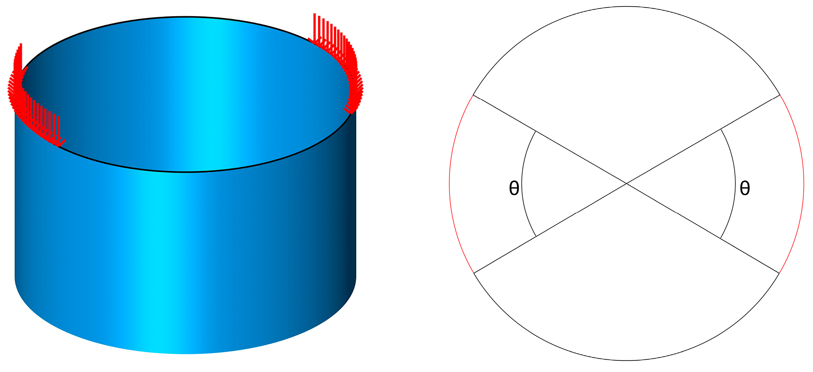
2.1. Circular Tube under Localized Axial Compression Loads

The research object of this paper is a thin-walled circular shell under axial compression loads. Figure 1 is a schematic diagram of a thin-walled circular shell under local axial compression loads. The left figure is a three-dimensional diagram of the circular tube, with red arrows representing the local axial compression loads exerted on the end face of the circular tube in a certain angle range. On the right are a top-down view of the circular tube, the black areas where it is not stressed, and the red areas representing the axial compression loads at an axial pressure angle of $2\times \theta$, which simulates the experiment in reference [12], by adding a convex flange with a certain angle to the top of the cylindrical shell, the specimen was subjected to the axial compression buckling test system.

The tube has a thickness of 1.2 mm, a diameter of 1000 mm, and a height of 600 mm, and is made of DC01 cold-rolled steel with an elastic modulus of 206 GPa and a yield strength of 158.7 MPa.

2.2. Governing Equations

Different from the FEM, the VFIFE discretizes the structure into finite particles to describe the deformation and motion of the structure under loads, and the mass (moment of inertia) of each particle is the point at which the structure is concentrated after equivalence. The motion of a particle is described by Newton’s second law:

$$M\ddot{\mathit{x}}+cM\dot{\mathit{x}}=F$$

(1)

$$I\ddot{\mathit{\theta }}+c_{\theta }I\dot{\mathit{\theta }}=F_{\theta }$$

(2)

where $M$ and $I$ are the mass and moment of the inertia matrix of the particle, $\ddot{\mathit{x}}$ and $\ddot{\mathit{\theta }}$ are the acceleration and angular acceleration of the particle, $\dot{\mathit{x}}$ and $\dot{\mathit{\theta }}$ are the velocity and angular velocity of the particle, and $F$ and $F_{\theta }$ are the resultant force and the external force on the particle. The damping of the particle on translational and rotational degrees of freedom are $c$ and $c_{\theta }$, and generally, the particle is damped the same in all directions.

Refer to the derivation of existing scholars, substituting Equations (1) and (2) into the central difference method, the particle motion formula can be obtained as follows:

$${\mathit{x}}_{n+1}=c_1(\frac{\Delta t^2}{\mathit{m}})F_n+2c_1{\mathit{x}}_n-c_2{\mathit{x}}_{n-1}$$

(3)

$${\mathit{\theta }}_{n+1}=c_1\Delta t^2{I}^{-1}{F}_{\theta n}+2c_1{\mathit{\theta }}_n-c_2{\mathit{\theta }}_{n-1}$$

(4)

where ${\mathit{x}}_n$ and ${\theta }_n$ are the position vector and the corner vector of the particle at step n, $F_n$ and $F_{\theta n}$ are the resultant force and resultant moment of the particle at step n, $\Delta t$ is the time step of a single loading step, and $c_1$ and $c_2$ are the constants associated with damping.

2.3. Internal Force

Unlike the FEM, which solves the internal force by solving linear equations, the VFIFE solves the internal force by decomposing the element displacement into the rigid body displacement and solving the internal force by using pure deformation through the virtual work principle.

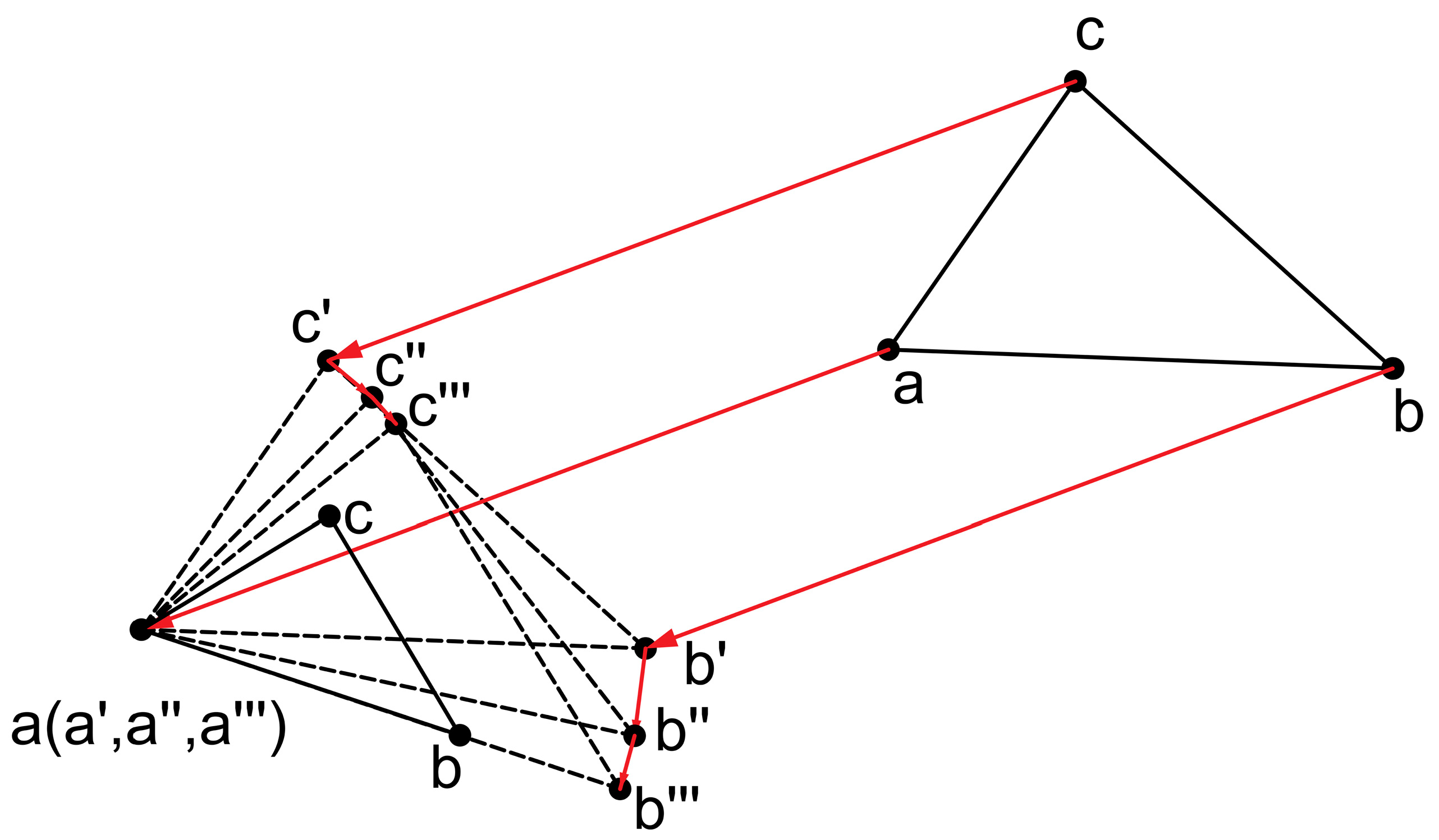
2.3.1. Inverse Motion

VFIFE solves the pure deformation of the structure by inverse motion. The inverse motion of a shell element is represented in Figure 2:

The inverse motion in space undergoes rigid body translation (abc→a’b’c’), out of the plane to inplane (a’b’c’→a’’b’’c’’), and rotation inplane (a’’b’’c’’→a’’’b’’’c’’’), and finally, the pure deformation of each particle on the element is obtained:

$$\left\{\begin{array}{l}\Delta {\mathit{\eta }}_{\mathrm{a}}^{\mathrm{d}}=0,\Delta {\mathit{\eta }}_i^{\mathrm{d}}=(u_i-u_a)+\Delta {\mathit{\eta }}_{i-op}^r+\Delta {\mathit{\eta }}_{i-ip}^r,i=b,c\\ \Delta {\mathit{\eta }}_{\theta i}^{\mathrm{d}}=u_{\theta i}+\Delta {\mathit{\eta }}_{\theta i-op}^r+\Delta {\mathit{\eta }}_{\theta i-ip}^r,i=a,b,c\end{array}\right.$$

(5)

where $\Delta {\mathit{\eta }}_i^{\mathrm{d}}$ and $\Delta {\mathit{\eta }}_{\theta i}^{\mathrm{d}}$ represent the pure deformation line displacement and angular displacement of the particle, $\Delta {\mathit{\eta }}_{i-op}^r$ and $\Delta {\mathit{\eta }}_{\theta i-op}^r$ represent the pure deformation line and angular displacements out of the plane, and $\Delta {\mathit{\eta }}_{i-ip}^r$ and $\Delta {\mathit{\eta }}_{\theta i-ip}^r$ represent the pure deformation line and angular displacements in the plane.

2.3.2. Solution of Internal Force

The internal force calculation on VFIFE is based on pure deformation by the virtual work principle. Through the virtual work principle, the internal forces at each node of the shell element can be obtained by linear superposition of the bending internal forces obtained by the DKT thin plate element and the tensile and compressive internal forces obtained by the CST membrane element. The internal forces are solved by the following formula:

$${{\displaystyle \sum _i\delta ({\widehat{\mathit{u}}}_i)}}^{\mathrm{T}}{\widehat{f}}_i+{{\displaystyle \sum _i\delta ({\widehat{\mathit{u}}}_{\theta i})}}^{\mathrm{T}}{\widehat{f}}_{\theta i}={\displaystyle \underset{\mathrm{V}}{\int }\delta {(\Delta {\widehat{\mathit{\epsilon }}}_m)}^{\mathrm{T}}{\widehat{\mathit{\sigma }}}_{m}dV}+{\displaystyle \underset{\mathrm{V}}{\int }\delta {(\Delta {\widehat{\mathit{\epsilon }}}_p)}^{\mathrm{T}}{\widehat{\mathit{\sigma }}}_{p}dV}$$

(6)

where $\Delta \widehat{\mathit{\epsilon }}$ and $\widehat{\mathit{\sigma }}$ represent the strain increment and stress of the node, respectively, and m stands for the membrane element and p for the plate element.

2.4. Determination of Buckling

This paper determines whether the structure is buckling according to the axial–force-displacement relationship. Before the structure buckling, the axial force gradually increases with the increase of displacement, with the two having a linear relationship. When the structure buckles, the axial force at the buckling point will decrease with the increase of displacement, and the axial force at the buckling point is considered as the buckling load of the structure. Due to the dynamic characteristics of the process of VFIFE analysis, the method of gradually increasing the axial force needs to wait until the result converges, which is not effective for the prediction of buckling. Therefore, the method of imposing forced displacement on the structure is adopted to push back the axial force of the structure, to draw the axial-force–displacement relationship curve of the buckling process. Formula (7) is the calculation formula of the axial force in reverse derivation:

$$\left\{\begin{array}{c}{\mathit{f}}_n^{ext}=\frac{1}{c_1\Delta t^2}M({\mathit{x}}_{n+1}+c_2{\mathit{x}}_{n-1}-2c_1{\mathit{x}}_n)-{\mathit{f}}_n^{\mathrm{int}}\\ {\mathit{f}}_{\theta n}^{ext}=\frac{1}{c_1\Delta t^2}M({\mathit{\theta }}_{n+1}+c_2{\mathit{\theta }}_{n-1}-2c_1{\mathit{\theta }}_n)-{\mathit{f}}_{\theta n}^{\mathrm{int}}\end{array}\right.$$

(7)

where ${\mathit{f}}_n^{ext}$ and ${\mathit{f}}_{\theta n}^{ext}$ represent the external force and moment of the particle at loading step n, and ${\mathit{f}}_n^{\mathrm{int}}$ and ${\mathit{f}}_{\theta n}^{\mathrm{int}}$ represent the internal force and internal moment of the particle at loading step n.

2.5. Nonlinearity

2.5.1. Geometric Nonlinearity

Based on Newton’s second law, VFIFE discretizes the structure into a finite number of particles to describe the deformation and motion state of the structure. The state of the structure is related to the velocity and acceleration direction of the particles under the force. The motion state of the points in the path element can be clearly described, so it is not necessary to correct the geometric nonlinearity of a structure with a large deformation and a large displacement.

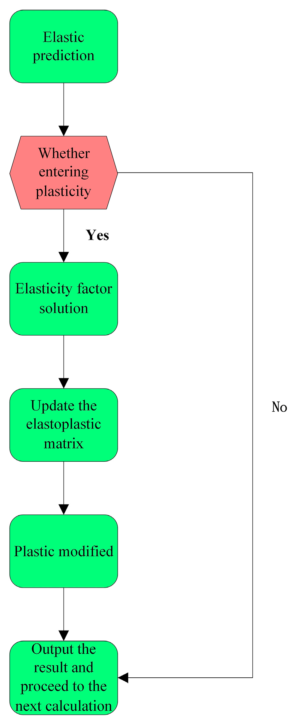
2.5.2. Material Nonlinearity

When the deformation is small, the material will recover its original state after the load is removed, so this stage belongs to the elastic stage of the material. When the deformation exceeds the range of elastic deformation, it will produce permanent deformation from which the material cannot recover. However, the stress–strain relationship of the material in the plastic stage is relatively complex, and the plasticity of the material in the numerical simulation is a material nonlinear problem, which requires a separate method to describe.

In the existing VFIFE study, there is only the bilinear hardening model and the power hardening model, which cannot accurately simulate the elastoplasticity of the materials. In order to accurately describe the strain state of the element under different stress states, a multilinear hardening model was used to discretize the material constitutive curve into multiple points, and the points were connected into broken lines. The elastic-plastic matrix under the state was updated according to the stress state of different load steps to accurately predict the elastic-plastic stress–strain of the material.

The von Mises yield criterion was used to judge whether it was plastic or not, and each integration layer is considered as a plane stress state while integrating according to thickness. When the stress satisfies the following formula,

$$F=\overline{\sigma }-{\sigma }_s^2=0$$

(8)

The material is considered to have reached the yield point, if F > 0, and the material enters the plastic stage. Equation (8), $\overline{\sigma }$ is equivalent to von Mises stress, and ${\sigma }_{\mathrm{s}}$ is the yield limit;

At time t, the strain increment $\Delta \mathit{\epsilon }$ can be calculated according to the existing node displacement. Assuming that the increment step is elastic, the stress increment can be calculated according to the existing strain increment, and the elastic predicted stress at a time $t+\Delta t$ can be calculated by superimposing the stress at time t, as shown in Equation (9),

$${}^{t+\Delta t}\mathit{\sigma }^{pr}={}^t\mathit{\sigma }+D_{\mathrm{e}}\Delta \mathit{\epsilon }$$

(9)

where ${}^{t+\Delta t}\mathit{\sigma }^{pr}$ represents elastic predictive stress at the time $t+\Delta t$, ${}^t\mathit{\sigma }$ represents the stress at time t, and $D_{\mathrm{e}}$ represents the elastic matrix;

The equivalent treatment of elastic predicted stress solved by the elastic prediction method is introduced into the von Mises yield formula. If the result is greater than zero, the node is in an elastic state and continues to be solved according to linear elasticity. If the result is less than zero, it means that it has entered a plastic state. Here, the elastic factor m, which is the proportion of elasticity at the integration point, is introduced. The solution of m is:

$$\mathrm{m}=(-a_1+\sqrt{a_1{}^2+4a_0{a}_2})/2a_2$$

(10)

where, for isotropic hardening materials, $a_0$ is the von Mises yield function at time t. Therefore, $a_1$ and $a_2$ are obtained by the following formula:

$$\left\{\begin{array}{l}{a}_1={\mathbf{S}}^{\mathrm{T}}\Delta \mathbf{S}\\ a_2=\frac{1}{2}\Delta {\mathbf{S}}^{\mathrm{T}}\Delta \mathbf{S}\end{array}\right.$$

(11)

where $\mathbf{S}$ presents the tensor of deviation stress at time t and $\Delta \mathbf{S}$ represents the increment of deviation stress at time t, and the superscript T stands for matrix transpose.

It should be noted that the m value calculated here should be greater than zero and less than one. If it is not in this interval, all the values are set as plastic, that is, m = 0;

The update of and material hardening modulus of the elastic-plastic matrix are closely related, and the mathematic expression of the hardening modulus is:

$${\mathit{E}}_p=\frac{\mathrm{E}{\mathrm{E}}_{\mathrm{t}}}{\mathrm{E}-{\mathrm{E}}_{\mathrm{t}}}$$

(12)

where ${\mathrm{E}}_{\mathrm{t}}$ represents the tangent modulus, which is the slope of the tangent at the point corresponding to the constitutive curve of the material under this stress state. The multilinear hardening model in this paper simplifies the constitutive curve of materials into multiple broken lines, and the tangent modulus is taken as the slope of the corresponding interval broken line on the simplified constitutive curve where the stress is at time $t-\Delta t$. At the same time, according to the flow rule of isotropic hardening, the hardening of materials can only go outward along the circular tangent line of von Mises stress, not inward, and the slope of the actual constitutive curve will be less than zero when it reaches tensile strength, and therefore, in this paper, the tangent modulus of the part with a slope less than zero in the constitutive curve is taken as 1000, which can not only ensure the continuous hardening of the material but also keep a small error with the actual material.

After solving the hardening modulus, the elastic-plastic matrix can be updated. The plastic matrix is calculated as follows:

$${\mathbf{D}}_{\mathrm{p}}=\frac{\mathrm{E}}{\mathrm{B}(1-v^2)}\left[\begin{array}{ccc}{({\mathrm{s}}_{\mathrm{x}}+v{\mathrm{s}}_{\mathrm{y}})}^2& ({\mathrm{s}}_{\mathrm{x}}+v{\mathrm{s}}_{\mathrm{y}})({\mathrm{s}}_{\mathrm{y}}+v{\mathrm{s}}_{\mathrm{x}})& (1-v)({\mathrm{s}}_{\mathrm{x}}+v{\mathrm{s}}_{\mathrm{y}}){\mathsf{\tau }}_{\mathrm{x}\mathrm{y}}\\ ({\mathrm{s}}_{\mathrm{x}}+v{\mathrm{s}}_{\mathrm{y}})({\mathrm{s}}_{\mathrm{y}}+v{\mathrm{s}}_{\mathrm{x}})& {({\mathrm{s}}_{\mathrm{y}}+v{\mathrm{s}}_{\mathrm{x}})}^2& (1-v)({\mathrm{s}}_{\mathrm{y}}+v{\mathrm{s}}_{\mathrm{x}}){\mathsf{\tau }}_{\mathrm{x}\mathrm{y}}\\ (1-v)({\mathrm{s}}_{\mathrm{x}}+v{\mathrm{s}}_{\mathrm{y}}){\mathsf{\tau }}_{\mathrm{x}\mathrm{y}}& (1-v)({\mathrm{s}}_{\mathrm{y}}+v{\mathrm{s}}_{\mathrm{x}}){\mathsf{\tau }}_{\mathrm{x}\mathrm{y}}& {(1-v)}^2{\mathsf{\tau }}_{\mathrm{x}\mathrm{y}}{}^2\end{array}\right]$$

(13)

where,

$$\mathrm{B}={\mathrm{s}}_{\mathrm{x}}{}^2+{\mathrm{s}}_{\mathrm{y}}{}^2+2\nu {\mathrm{s}}_{\mathrm{x}}{\mathrm{s}}_{\mathrm{y}}+2(1-\nu ){\mathsf{\tau }}_{\mathrm{x}\mathrm{y}}{}^2+\frac{2(1-\nu ){\mathrm{E}}_p{\sigma }_{\mathrm{s}}}{9\mathrm{G}}$$

(14)

In the formula, G is the shear modulus and ${\mathrm{s}}_{\mathrm{x}}$ and ${\mathrm{s}}_{\mathrm{y}}$ is the deviation stress.

After the plastic matrix is calculated, the elastic-plastic matrix can be calculated:

$${\mathbf{D}}_{ep}={\mathbf{D}}_e-{\mathbf{D}}_p$$

(15)

First, calculate the plastic strain increment according to the strain increment

$$\Delta {\mathit{\epsilon }}_p=(1-\mathrm{m})\Delta \mathit{\epsilon }$$

(16)

Finally, the plastic stress is calculated:

$${}^{\mathrm{t}+\Delta \mathrm{t}}\mathit{\sigma }={}^{\mathrm{t}}\mathit{\sigma }+{\mathrm{m}}^{\mathrm{t}+\Delta \mathrm{t}}{\mathit{\sigma }}^{pr}+{\mathbf{D}}_{ep}\Delta {\mathit{\epsilon }}_p$$

(17)

Based on the VFIFE principles, the buckling program of the thin-shell structure is compiled, and the model data, boundary conditions, and loads are input into the calculation program. In each analysis step, the element displacement and internal force are calculated first, and then the equivalent stress and strain are calculated and introduced into the subprogram of the multilinear hardening model. First, the elastic prediction is carried out to determine whether the plastic stage has been entered, and if it has entered into the plastic stage, plastic correction is required. Finally, the next analysis step is carried out. The program flow of each elastic-plastic incremental step is shown in Figure 3.

3. Model Verification and Parameter Setting

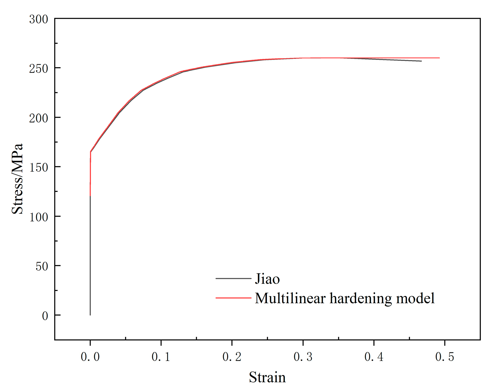
3.1. Multilinear Hardening Model Verification

To verify the feasibility of the multilinear hardening model, the axial tensile process of cold-rolled steel was simulated by an analysis program, and the simulated stress–strain curve was compared with the experimental stress–strain curve. The simulation material selected was DC01 cold rolled steel, with an elastic modulus of E = 206 GPa, a yield strength of ${\sigma }_s$ = 158.7 MPa, and an established specimen model, as shown in Figure 4. The simulation results were compared with the tensile test results [12]. To simulate the situation close to the test, the bottom of the specimen was fixed, and the top of the specimen was restricted except for the degree of freedom in the tensile direction. A forced upward displacement was applied to the top of the specimen. The stress–strain curve drawn by taking the equivalent stress–strain of the central node of the specimen was compared with the test results, as shown in Figure 5.

It can be seen from the above comparison results that the simulation results are in good agreement with the experimental results, which proves that the multilinear hardening model introduced in this paper can accurately predict the stress value of the material under a given strain in the VFIFE.

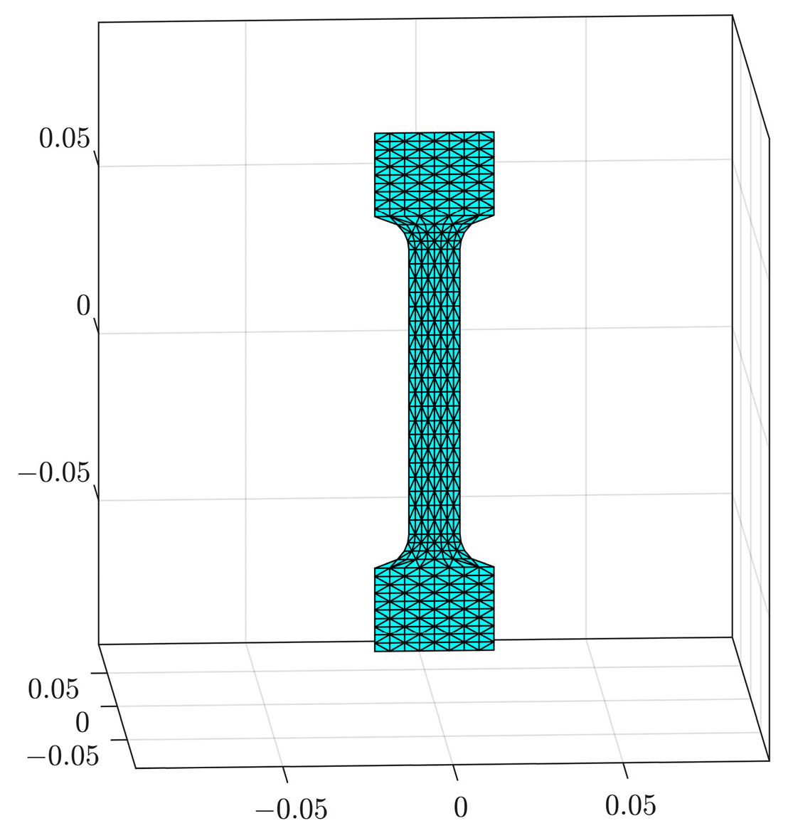
3.2. Calculation Parameters

Based on the above description, the buckling behavior of a circular tube under local axial compression is simulated by the VFIFE method. The axial compression of the structure is derived by applying the forced displacement, that is, a fixed constraint is applied to the bottom node of the tube, and a forced axial displacement is applied to the top node, limiting the other degrees of freedom except the forced axial displacement. The time step is $\Delta t=1\times 10^{-6}\mathrm{s}$. The multilinear hardening model is adopted. The material of the tube is DC01 cold-rolled steel, and the material parameters are set according to the test in Section 3.1.

A triangular shell element is adopted for the circular tube model. As shown in Figure 6, the element is discretized into three mass points distributed at the element nodes. Each triangular element is an isosceles right triangle.

Based on the analysis of the buckling load of a thin-walled circular shell under a 2 × 90° local axial compression load under different mesh sizes, the appropriate mesh is determined. The simulation calculation refers to the experimental setting of Jiao [12], with triangular meshes with side lengths of 20 mm, 30 mm, 40 mm, and 50 mm were analyzed respectively, loaded at 2 mm/s. The simulation and experimental errors obtained are shown in

Table 1. Buckling loads and errors were calculated from the mesh of different sizes.

Meshing Size/mm	Buckling Load/kN	Error/%
50	272.7	5.50
40	263.6	2.24
30	258.6	0.35
20	258.1	0.15

.

In the experiment, the first buckling load is 257.7 kN, as can be seen in Table 1, when the mesh size is 30 mm, the calculation error becomes small and the margin of error decreases slightly as the mesh size decreases, so the mesh size in this paper is 30 mm.

The forced displacement of the top node needs to be loaded at a certain speed, and the loading speed will affect the calculation results. The axial force–displacement curves at different speeds are analyzed, the optimal loading speed is selected by comparison., and the loading angle is 2 × 90°, with a triangular shell element, and the length of the right angle side of the element is 30 mm, loaded the top displacement at the speeds of 30 mm/s, 10 mm/s, 2 mm/s, and 1 mm/s, respectively, and the calculated displacement axial force curve is shown in Figure 7.

In the experiment, the first buckling load is 257.7 kN, and the first buckling load loaded at 30 mm/s is 265.6 kN, with an error of 3.07%, the first buckling load loaded at 10 mm/s is 263.6 kN, with an error of 2.28%, the first buckling load loaded at 2 mm/s is 258.6 kN, with an error of 0.34%, and the first buckling load loaded at 1 mm/s is 256.9 kN, with an error of 0.31%. It can be seen from the analysis results that before the buckling of the structure, each loading rate can be very close to the experimental results. However, due to the influence of inertial force, a faster loading rate means a greater buckling load. When the loading rate is reduced to 2 mm/s, the agreement between the first buckling load and the experiment reaches a relatively ideal level, however, there is still a large gap between the subsequent curve and the experiment. After loading at the rate of 1 mm/s, the result is improved, so this paper adopted the rate of 1 mm/s for loading.

It should be pointed out that there are often many small gaps between the experimental process and the expected design, such as the initial defects of the specimen and the uneven control of the load. These conditions are in an ideal state in the numerical simulation, and the small gap between the two will cause non-negligible errors in the buckling structure. For the subsequent buckling behavior after the first buckling, it is very difficult to simulate results that are very consistent with the experiment. However, if subsequent buckling similar to the experiment can be simulated, it has a very important value for guiding the structural design.

4. Results and Discussion

In this paper, based on the simulation program, buckling loads under different degrees of local axial compression are calculated, and the buckling modes are predicted. Finally, postbuckling is visualized by drawing a displacement contour of the tube at different stages in the deformation process, and the development of buckling under local axial compression load is explored.

4.1. First Buckling Load Buckling Modes

Simulations were performed for circular tubes with axial compression angles of 2 × 30°, 2 × 60°, 2 × 90°, 2 × 120°, 2 × 150°, and 2 × 180° (overall axial compression), and the calculated results were plotted as displacement–axial force curves to compare with the experimental results, as shown in Figure 8.

Table 2. Comparison of results.

Axial Compression Angle	Experiment/kN	VFIFE/kN	Error/%
2 × 30°	138.9	137.9	0.72
2 × 60°	191.0	192.3	0.68
2 × 90°	257.7	256.9	0.31
2 × 120°	310.3	313.1	0.99
2 × 150°	409.1	406.3	0.68
2 × 180°	466.3	468.4	0.45

shows the comparison between the first buckling load calculated by VFIFE and the experiments in the literature. The error between the first buckling load predicted by VFIFE and the experimental results is less than 1%.

When the angle of local axial comparison is 2 × 30°, 2 × 60°, 2 × 90°, and 2 × 120°, secondary buckling occurs in both the experimental and the simulation results, as seen in the abrupt change of the displacement-axial force curve in Figure 9. VFIFE predicts four buckling of the structure for a local axial comparison angle of 2 × 30°, two buckling for local axial comparison angles of 2 × 60°, 2 × 90°, and 2 × 120°, and only one buckling for axial comparison angles of 2 × 150° and 2 × 180°. It is inferred that the smaller the local axial comparison angle, the more likely the structure is to buckle several times, so every engineering project should try to avoid a local axial pressure load on the circular tube.

The prediction of modal and postbuckling behavior of thin-shell structure buckling has far-reaching significance for practical engineering. The FEM prediction of postbuckling buckling is done by first solving a linear equation system, then calculating different modal orders according to different eigenvalues, and then adding different modalities to the structure according to geometric defects, all in order to predict the postbuckling behavior of the structure, which is a complicated process to solve. VFIFE with its dynamic solution predicts the buckling behavior of thin-shell structures after buckling without additional modal analysis operations and predicts the structural modalities at different stages of buckling and accurately predicts the loads in this state.

Table 3. Comparison of buckling mode. Pictures of the experiment are reproduced with the permission of [12], copyright@Thin-Walled Structures, 2021.

Angle	Experiment	VFIFE
2 × 90°
2 × 120°
2 × 180°

shows the comparison between the buckling modes calculated by VFIFE near the first buckling of the circular tube under 2 × 90° and 2 × 120° local axial compression loads, and 2 × 180° overall axial compression load, and the experimental results [12]. In the table, the buckling modes calculated by VFIFE are represented by a displacement contour, in which the color bar from blue to red represents the change of the overall displacement from large to small, and the buckling deformation is generally larger, and it is easy to distinguish the deformation direction, so deformation size is taken as an absolute value.

Based on the buckling modes near the first buckling, it can be seen that the location and deformation of the buckling deformation calculated by VFIFE are more similar to the experiments, and the predictions of the buckling deformation of the thin-shell structure by VFIFE are more appropriate to the actual situation.

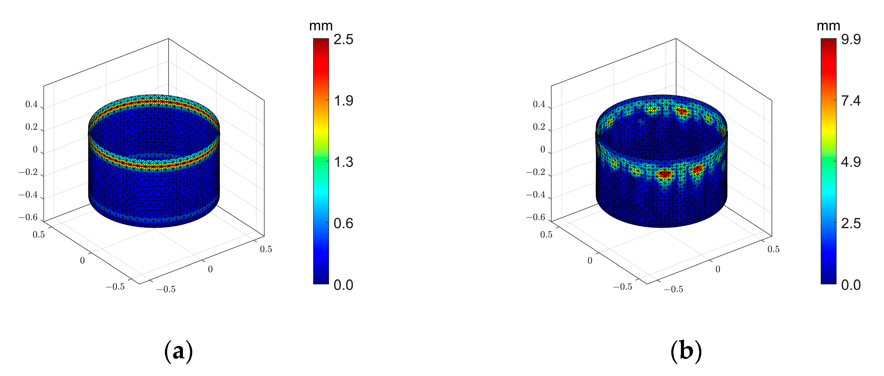
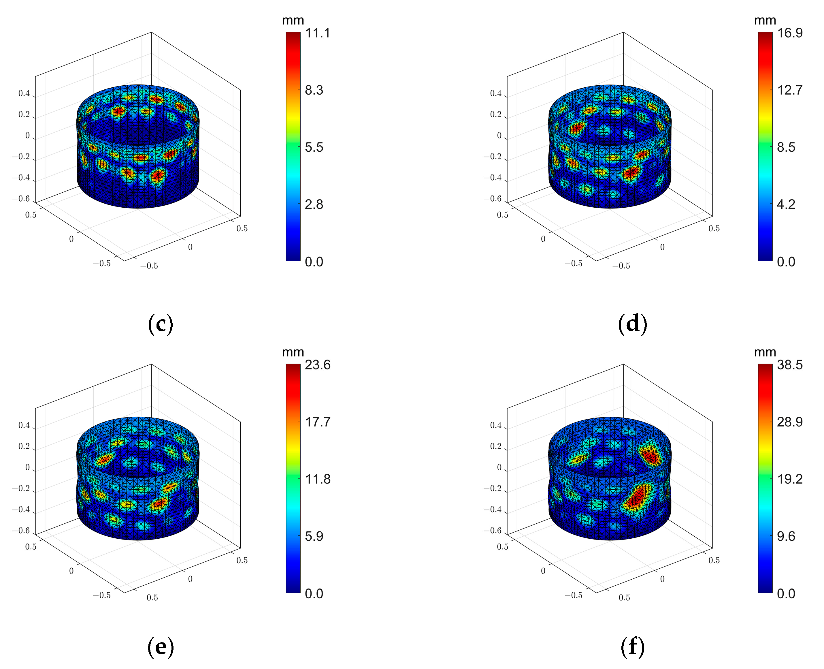
4.2. Buckling Modes and Postbuckling

The calculation of the first buckling load is of great value for guiding the structural design, however, it is still difficult to avoid buckling of the structure in actual engineering. The prediction of the postbuckling behavior of the structure is also of high value for guiding engineering. Most commercial software based on FEM can solve the structural buckling load by solving linear equations with the eigenvalue method and solve the postbuckling modes by the explicit dynamics method, though the process is cumbersome, and VFIFE can do these calculations directly. According to previous studies, the validity and accuracy of the VFIFE method proposed in this paper are verified in the buckling analysis of thin-walled circular shells. Based on developed analytical procedures, this section investigates the postbuckling behavior of thin-walled circular shells.

The postbuckling behavior under local axial compression load was analyzed, and the postbuckling of 2 × 90° local axial compression and 2 × 120° local axial compression were analyzed, respectively. The forced displacement of 8 mm downward was applied to the end of the pipe through different local axial compression angles, and the postbuckling behavior was studied according to the displacement contour after deformation, with the color in the displacement contour the same as in Section 3, the blue to red representing the change of the total displacement from large to small, and the deformation size is taken as an absolute value.

Figure 9 depicts the postbuckling of the circular tube under the local axial compression load of 2 × 90°. Figure 9a–e is the unified view angle, and in Figure 9f, the view angle is adjusted to the side of the axial compression applied more conveniently. Figure 9a shows the state of the structure when buckling is about to occur, under a local axial compression load of 2 × 90°, the figure shows that the locations where obvious folds appear were not under compression, and the larger deformations occur in the regions outside the axial compression locations where folds appear. Figure 9b,c are after the first buckling occurs, as the second buckling of the structure appears and develops, and the third buckling occurs in Figure 9d,e, where the depression deformation only becomes larger inward, no new depressions appear, and there is no load position where the fold of the structure gradually becomes larger. Similar to the overall axial compression, depressions still occur in the structure from above and downwards, however, the depressions only occur near the axial compression load. Figure 9f is the state of the structure after the 8 mm forced displacement is applied, the depression finally closes and occurs at the location of the axial compression load, and the rest is folded deformation. It can be predicted that if the load continues to be applied to it, the depression deformation at the position where the forced displacement is applied and the fold at the position where the load is not applied will continue to increase, and eventually, all the deformation will coincide, and then new deformation or even structural fracture may occur.

Figure 10 depicts the postbuckling of the circular tube under a local axial compression load of 2 × 120°. Figure 10a shows the state of the structure when buckling is about to occur, and the location where a clear fold appears can be seen in the figure as being without pressure, Figure 10b shows the depressed deformation of the structure after the first buckling, Figure 10b–d show the second buckling of the structure, and the deformations are developing and tend to merge, Figure 10e shows the third buckling of the structure, however, the buckling deformation is smaller than the first two bucklings, and Figure 10f shows the state of the structure after 8 mm forced displacement is applied, as the depressions finally merge and occur at the locations of the axial compression load, while at the locations without axial compression load, the structure has a large inward fold, and the deformation of the structure is already very serious at this time. As can be seen from the postbuckling of 2 × 90° local axial compression, the development of buckling is very similar to the postbuckling of 2 × 90° local axial compression and folds appear in areas where no axial compression is applied before buckling occurs. When the fold continues to expand after buckling, depression deformation occurs at the location where the axial compression is applied.

Finally, the postbuckling behavior of overall axial compression is simulated as a control, and the postbuckling of the circular tube is achieved by applying a forced axial displacement of 8 mm downward from the end of the tube to the circular tube. Figure 11 is the displacement contour of the structure in the whole loading process after buckling, Figure 11a shows that the first buckling occurs just at the beginning, the element extrusion deformation first appears at the location where the depression is about to occur, Figure 11b depicts the gradual formation of the depression at the extrusion location to the inside of the tube, the deformation of the depression gradually expands and then the second buckling appears at Figure 11c and the third buckling at Figure 11d. At this time, the depression formed by the third buckling has covered the entire round tube. The deformation of the depression in Figure 11e gradually increases and eventually merges into a larger depression in Figure 11f, and as the buckling deformation continues to develop, contact between elements will appear. At this time, boundary nonlinearity needs to be introduced. The shell element adopted in this paper does not include boundary nonlinearity and fracture determination, so subsequent developments are not within the scope of this paper.

The three examples of postbuckling above show that a circular tube subjected to axial compression loading will deform in a top-down depression after buckling occurs. Compared with the overall axial compression, the deformation of the local axial compression circular tube is more irregular, the deformation of the region under load is mostly an inward sag, the region without axial compression will fold, and the fold will gradually increase with the axial displacement, resulting in the shape of the top of the circular tube becoming irregular, and as the mechanical characteristics of such irregular shapes are difficult to predict, such phenomenon should be avoided as much as possible in practical engineering.

5. Conclusions

Based on the vector form intrinsic finite element theory, this paper developed a program for calculating and analyzing the buckling of the structure, considering the multilinear hardening model, verified the multilinear hardening model according to the experimental data, and then simulated the buckling of a thin-walled circular shell under a local axial compression load. Compared with the experimental results, the postbuckling behavior of the thin-walled circular shell was as predicted. The following conclusions can be drawn:

(1)

The multilinear hardening model based on the von Mises yield criterion can divide the elastic-plastic constitutive curve of materials into multiple broken lines and can approach the elastic-plastic constitutive curve of some materials infinitely closely. The stress–strain relationship of materials can be simulated accurately when the model is applied to VFIFE. Compared with the ideal elastoplasticity, bilinear hardening model, power hardening model, and Ramberg–Osgood model used in most numerical simulations, the structural strain under a given stress can be simulated more accurately.

(2)

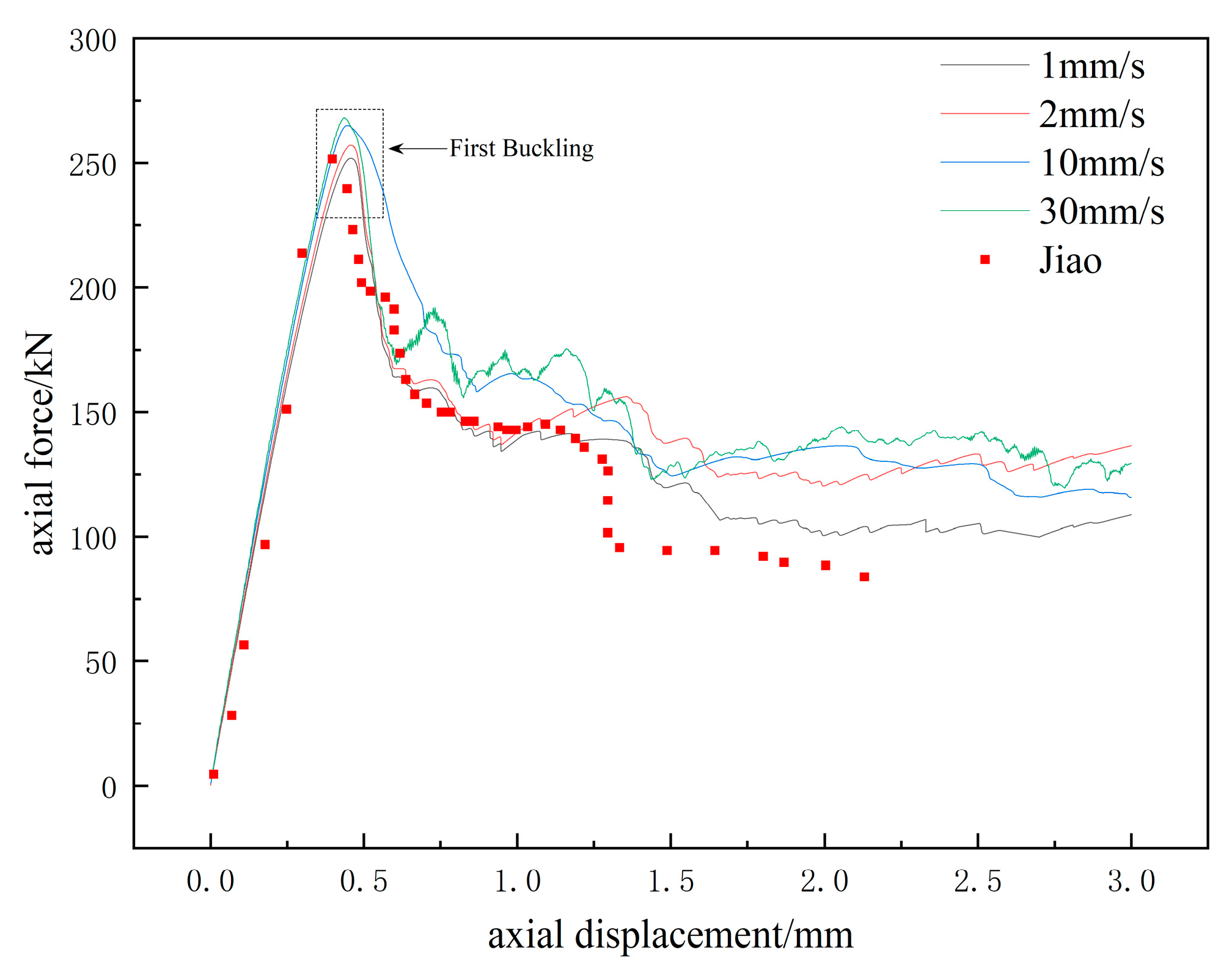
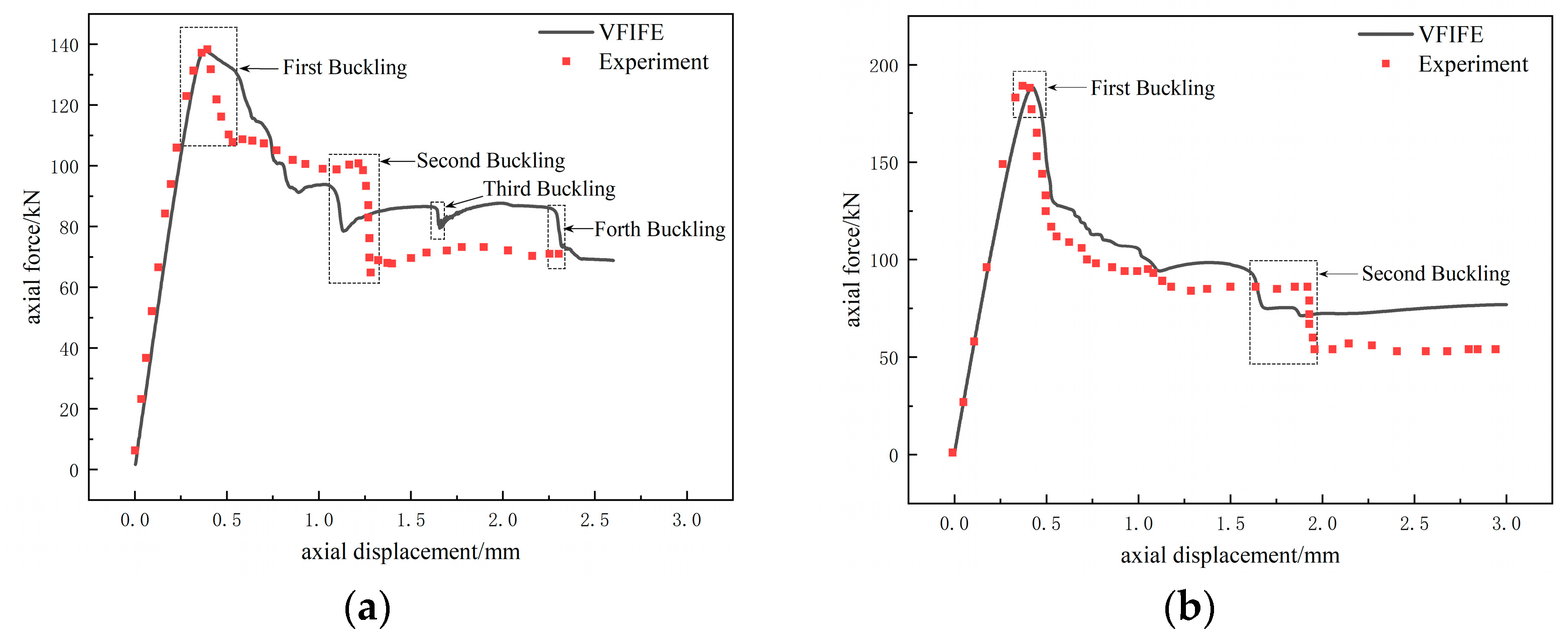
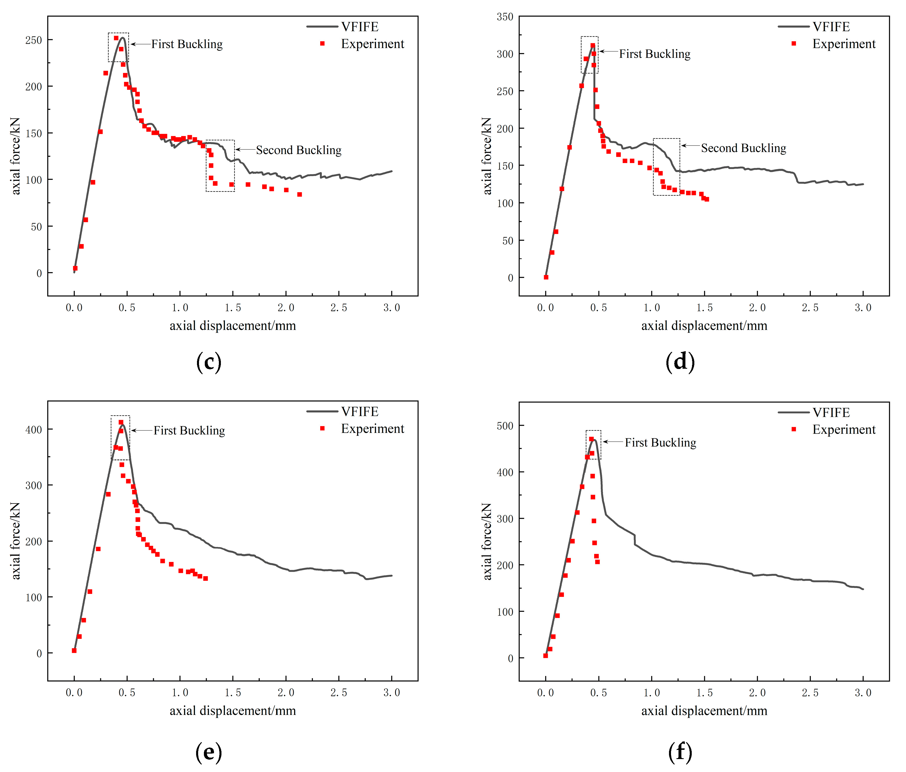
The VFIFE introduces the multilinear hardening model, which predicts the first buckling load of the local axial compression tube with high accuracy, and the error between the simulation and experiment in this paper is less than 1%. For the buckling mode, after the first buckling occurs, the results of the VFIFE simulation are more consistent with the experiment, which verifies the effectiveness and accuracy of VFIFE in predicting structural buckling.

(3)

For the prediction of the postbuckling of structures, VFIFE has great advantages. Different from the complex settings of most commercial software based on FEM, VFIFE can directly predict the postbuckling behavior of structures under the action of force.

(4)

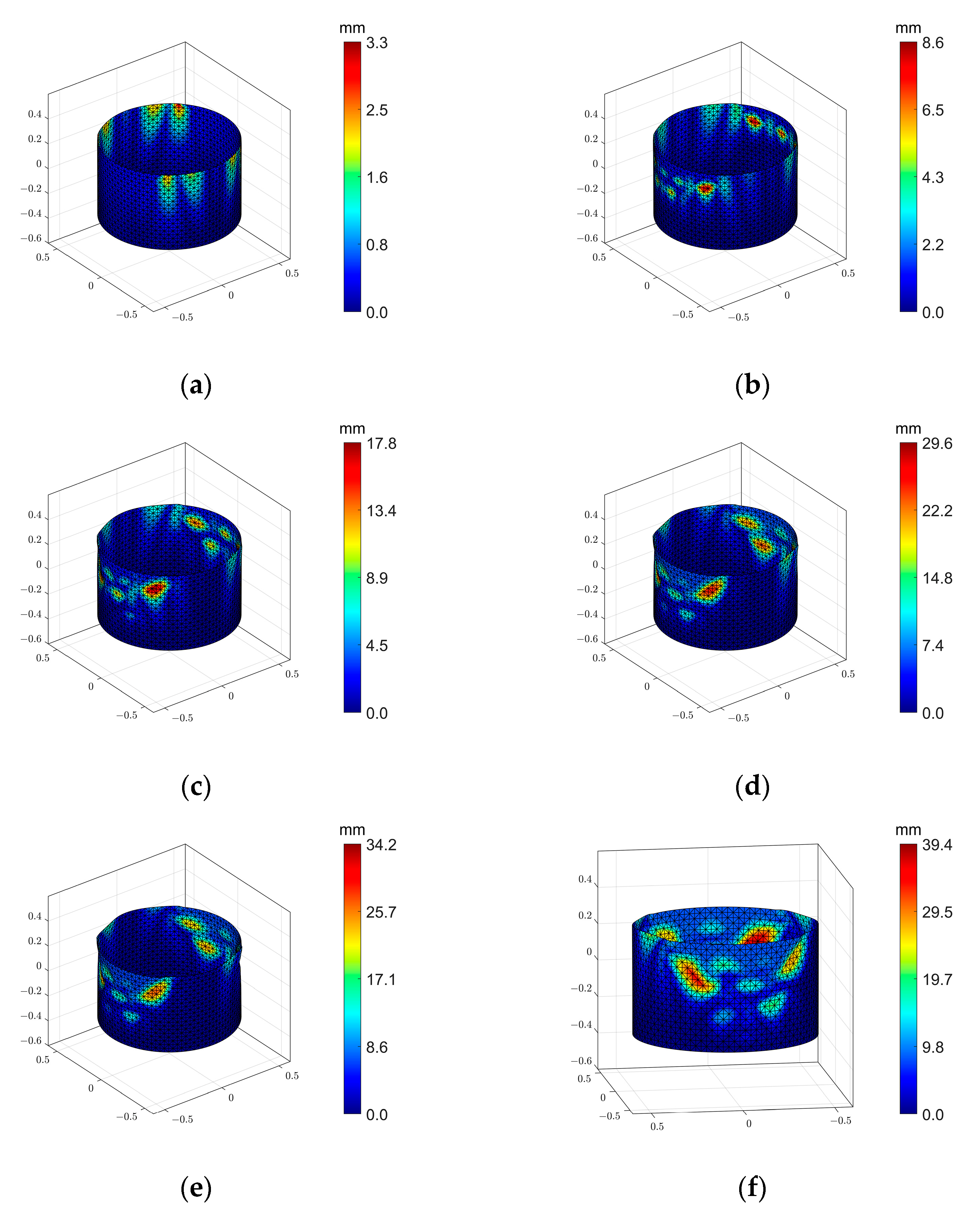
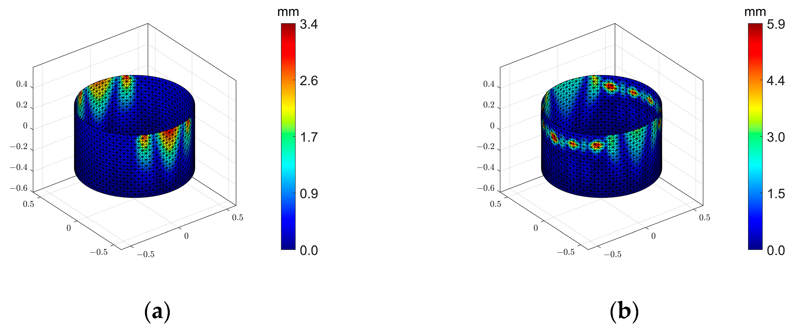
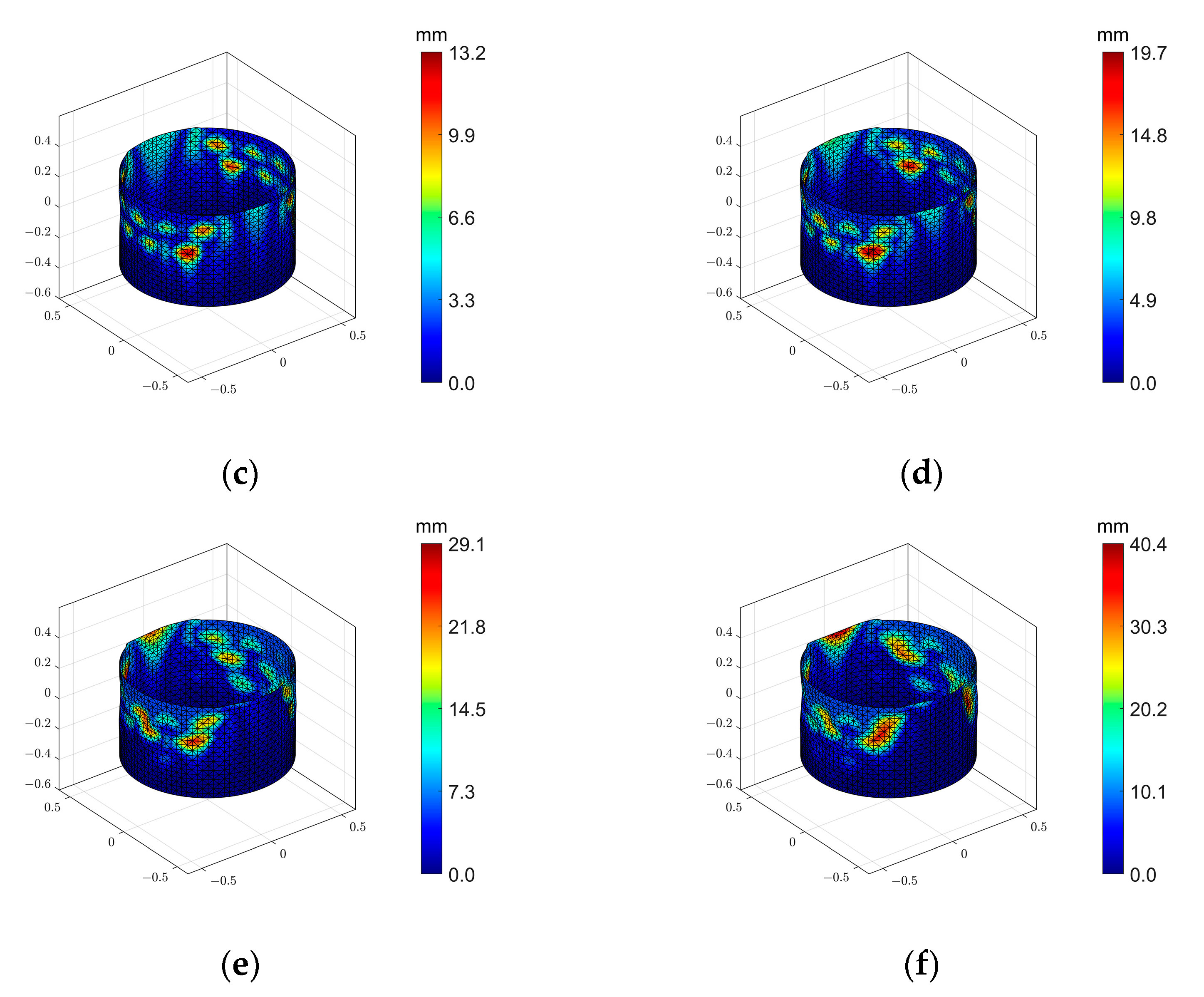
When a circular tube is subjected to local axial compression loads, the smaller the local axial compression angle, the smaller the buckling load will be. If the load is in the form of overall axial compression, the depression deformation will appear uniformly along the circular tube ring, while if the load is in the form of local axial compression, the depression will occur at the location of the load, and the rest of the location of the fold, so that the geometry of the force side of the circular tube becomes irregular, affecting the mechanical properties of the structure. Such situations should be avoided in engineering wherever possible.

References

1. Wagner, H.N.R.; Hühne, C. Robust knockdown factors for the design of cylindrical shells under axial compression: Potentials, practical application and reliability analysis. Int. J. Mech. Sci. 2018, 135, 410–430. [Google Scholar] [CrossRef]
2. Trivedi, N.; Singh, R.K. Fracture characterization studies of concrete structures through experiments on reinforced concrete cylindrical shell specimens. Ann. Nucl. Energy 2020, 140, 107338. [Google Scholar] [CrossRef]
3. Su, R.; Li, X.; Xu, S.-Y. Axial behavior of circular CFST encased seawater sea-sand concrete filled PVC/GFRP tube columns. Construct. Build. Mater. 2022, 353, 129159. [Google Scholar] [CrossRef]
4. Chung, C.-C.; Lee, K.-L.; Pan, W.-F. Collapse of Sharp-Notched 6061-T6 Aluminum Alloy Tubes under Cyclic Bending. Int. J. Struct. Stab. Dyn. 2016, 16, 1550035. [Google Scholar] [CrossRef]
5. Horrigmoe, G.; Bergan, P.G. Nonlinear analysis of free-form shells by flat finite elements. Comput. Methods Appl. Mech. Eng. 1978, 16, 11–35. [Google Scholar] [CrossRef]
6. Combescure, A.; Galletly, G.D. Plastic buckling of complete toroidal shells of elliptical cross-section subjected to internal pressure. Thin-Walled Struct. 1999, 34, 135–146. [Google Scholar] [CrossRef]
7. Spagnoli, A.; Chryssanthopoulos, M.K. Elastic buckling and postbuckling behaviour of widely-stiffened conical shells under axial compression. Eng. Struct. 1999, 21, 845–855. [Google Scholar] [CrossRef]
8. Abambres, M.; Camotim, D.; Silvestre, N. GBT-based elastic–plastic post-buckling analysis of stainless steel thin-walled members. Thin-Walled Struct. 2014, 83, 85–102. [Google Scholar] [CrossRef]
9. Kadkhodayan, M.; Maarefdoust, M. Elastic/plastic buckling of isotropic thin plates subjected to uniform and linearly varying in-plane loading using incremental and deformation theories. Aerosp. Sci. Technol. 2014, 32, 66–83. [Google Scholar] [CrossRef]
10. Song, C.Y.; Teng, J.G.; Rotter, J.M. Imperfection sensitivity of thin elastic cylindrical shells subject to partial axial compression. Int. J. Solids Struct. 2004, 41, 7155–7180. [Google Scholar] [CrossRef]
11. Changyong, S. Buckling of un—Stiffened cylindrical shell under non—Uniform axial compressive stress. J. Zhejiang Univ. Sci. 2002, 3, 520–531. [Google Scholar] [CrossRef]
12. Jiao, P.; Chen, Z.; Ma, H.; Ge, P.; Gu, Y.; Miao, H. Buckling behaviors of thin-walled cylindrical shells under localized axial compression loads, Part 1: Experimental study. Thin-Walled Struct. 2021, 166, 108118. [Google Scholar] [CrossRef]
13. Jiao, P.; Chen, Z.; Ma, H.; Ge, P.; Gu, Y.; Miao, H. Buckling behaviors of thin-walled cylindrical shells under localized axial compression loads, Part 2: Numerical study. Thin-Walled Struct. 2021, 169, 108330. [Google Scholar] [CrossRef]
14. Nassiraei, H.; Zhu, L.; Gu, C. Static capacity of collar plate reinforced tubular X-connections subjected to compressive loading: Study of geometrical effects and parametric formulation. Ships Offshore Struct. 2019, 16, 54–69. [Google Scholar] [CrossRef]
15. Nassiraei, H.; Rezadoost, P. Static capacity of tubular X-joints reinforced with fiber reinforced polymer subjected to compressive load. Eng. Struct. 2021, 236, 112041. [Google Scholar] [CrossRef]
16. Wu, C.; Lou, J.; He, L.; Du, J.; Wu, H. Buckling and Post-Buckling of Symmetric Functionally Graded Microplate Lying on Nonlinear Elastic Foundation Based on Modified Couple Stress Theory. Int. J. Struct. Stab. Dyn. 2018, 18, 1850110. [Google Scholar] [CrossRef]
17. Liu, X.; Zhang, J.; Di, C.; Zhan, M.; Wang, F. Buckling of Hydroformed Toroidal Pressure Hulls with Octagonal Cross-Sections. Metals 2022, 12, 1475. [Google Scholar] [CrossRef]
18. Peng, Y.; Kong, Z.; Dinh, B.H.; Nguyen, H.-H.; Cao, T.-S.; Papazafeiropoulos, G.; Vu, Q.-V. Web Bend-Buckling of Steel Plate Girders Reinforced by Two Longitudinal Stiffeners with Various Cross-Section Shapes. Metals 2023, 13, 323. [Google Scholar] [CrossRef]
19. Barham, W.S.; Idris, A.A. Flexibility-based large increment method for nonlinear analysis of Timoshenko beam structures controlled by a bilinear material model. Structures 2021, 30, 678–691. [Google Scholar] [CrossRef]
20. Zhang, C.; Yang, X. Bilinear elastoplastic constitutive model with polyvinyl alcohol content for strain-hardening cementitious composite. Constr. Build. Mater. 2019, 209, 388–394. [Google Scholar] [CrossRef]
21. Turkalj, G.; Lanc, D.; Brnic, J. Large displacement beam model for creep buckling analysis of framed structures. Int. J. Struct. Stab. Dyn. 2009, 9, 61–83. [Google Scholar] [CrossRef]
22. Xiao, G.; Yang, X.; Qiu, J.; Chang, C.; Liu, E.; Duan, Q.; Shu, X.; Wang, Z. Determination of power hardening elastoplastic constitutive relation of metals through indentation tests with plural indenters. Mech. Mater. 2019, 138, 103173. [Google Scholar] [CrossRef]
23. Lu, X.; Huang, F.; Zhao, B.; Keer, L.M. Contact Behaviors of Coated Asperity with Power-Law Hardening Elastic–Plastic Substrate During Loading and Unloading Process. Int. J. Appl. Mech. 2018, 10, 1850034. [Google Scholar] [CrossRef]
24. Chen, L.; Yu, Y.; Song, W.; Wang, T.; Sun, W. Stability of geometrically imperfect struts with Ramberg-Osgood constitutive law. Thin-Walled Struct. 2022, 177, 109438. [Google Scholar] [CrossRef]
25. Huang, Z.; Chen, Y.; Bai, S.-L. An Elastoplastic Constitutive Model for Porous Materials. Int. J. Appl. Mech. 2013, 5, 50035. [Google Scholar] [CrossRef]
26. Mourlas, C.; Khabele, N.; Bark, H.A.; Karamitros, D.; Taddei, F.; Markou, G.; Papadrakakis, M. Effect of Soil–Structure Interaction on Nonlinear Dynamic Response of Reinforced Concrete Structures. Int. J. Struct. Stab. Dyn. 2020, 20, 2041013. [Google Scholar] [CrossRef]
27. Ruocco, E.; Reddy, J.N. Buckling analysis of elastic–plastic nanoplates resting on a Winkler–Pasternak foundation based on nonlocal third-order plate theory. Int. J. Non-Linear Mech. 2020, 121, 103453. [Google Scholar] [CrossRef]
28. Zhou, W.; Shi, Z.; Li, Y.; Rong, Q.; Zeng, Y.; Lin, J. Elastic-plastic buckling analysis of stiffened panel subjected to global bending in forming process. Aerosp. Sci. Technol. 2021, 115, 106781. [Google Scholar] [CrossRef]
29. Zou, Z.; Liu, D.; Song, C.; Jin, M.; Guo, B.; Zhang, H. Elastic-Plastic Finite Element New Method for Lower Bound Shakedown Analysis. Int. J. Struct. Stab. Dyn. 2022, 22, 2250171. [Google Scholar] [CrossRef]
30. Shih, C.; Wang, Y.-K.; Ting, E.C. Fundamentals of a Vector Form Intrinsic Finite Element: Part III. Convected Material Frame and Examples. J. Mech. 2011, 20, 133–143. [Google Scholar] [CrossRef]
31. Ting, E.C.; Shih, C.; Wang, Y.-K. Fundamentals of a Vector Form Intrinsic Finite Element: Part I. Basic Procedure and A Plane Frame Element. J. Mech. 2011, 20, 113–122. [Google Scholar] [CrossRef]
32. Ting, E.C.; Shih, C.; Wang, Y.-K. Fundamentals of a Vector Form Intrinsic Finite Element: Part II. Plane Solid Elements. J. Mech. 2011, 20, 123–132. [Google Scholar] [CrossRef]
33. Wu, H.; Zeng, X.; Xiao, J.; Yu, Y.; Dai, X.; Yu, J. Vector form intrinsic finite-element analysis of static and dynamic behavior of deep-sea flexible pipe. Int. J. Nav. Archit. Ocean Eng. 2020, 12, 376–386. [Google Scholar] [CrossRef]
34. Wu, T.-Y.; Ting, E.C. Large deflection analysis of 3D membrane structures by a 4-node quadrilateral intrinsic element. Thin-Walled Struct. 2008, 46, 261–275. [Google Scholar] [CrossRef]
35. Wu, T.-Y. Dynamic nonlinear analysis of shell structures using a vector form intrinsic finite element. Eng. Struct. 2013, 56, 2028–2040. [Google Scholar] [CrossRef]
36. Zhen, W.; Yang, Z.; Xuelin, Y. Nonlinear behavior analysis of entity structure based on vector form intrinsic finite element. J. Build. Struct. 2015, 36, 133–140. [Google Scholar] [CrossRef]
37. Wu, T.-Y.; Tsai, W.-C.; Lee, J.-J. Dynamic elastic–plastic and large deflection analyses of frame structures using motion analysis of structures. Thin-Walled Struct. 2009, 47, 1177–1190. [Google Scholar] [CrossRef]
38. Zhen, W.; Yang, Z.; Xuelin, Y. Collision-contact, crack-fracture and penetration behavior analysis of thin-shell structures based on vector form intrinsic finite element. J. Build. Struct. 2016, 37, 53–59. [Google Scholar] [CrossRef]
39. Zhen, W.; Yang, z.; Xuelin, Y. Vector form intrinsic finite element method for buckling analysis of thin-shell structures. J. Cent. South Univ. (Sci. Technol.) 2016, 47, 2058–2064. [Google Scholar]
40. Zhen, W.; Yang, Z.; Xuelin, Y. Analisis of buckling behavior of planar membrane structures based on vector form intrinsic finite element. J. Zhejiang Univ. (Eng. Sci.) 2015, 49, 1116–1122. [Google Scholar]
41. Xu, L.; Lin, M. Analysis of buried pipelines subjected to reverse fault motion using the vector form intrinsic finite element method. Soil Dyn. Earthq. Eng. 2017, 93, 61–83. [Google Scholar] [CrossRef] [Green Version]
42. Yu, Y.; Li, Z.; Yu, J.; Xu, L.; Zhao, M.; Cui, Y.; Wu, H.; Duan, Q. Buckling analysis of subsea pipeline with integral buckle arrestor using vector form intrinsic finite thin shell element. Thin-Walled Struct. 2021, 164, 107533. [Google Scholar] [CrossRef]
43. Yu, Y.; Li, Z.; Yu, J.; Xu, L.; Cheng, S.; Wu, J.; Wang, H.; Xu, W. Buckling failure analysis for buried subsea pipeline under reverse fault displacement. Thin-Walled Struct. 2021, 169, 108350. [Google Scholar] [CrossRef]
44. The OpenMP API Specification for Parallel Programming. Available online: https://www.openmp.org (accessed on 1 June 2022).
Figure 1. Tube under localized axial compression loads.
Metals 13 00564 g001
Figure 2. Inverse motion of a shell element.
Metals 13 00564 g002
Figure 3. Multilinear hardening model program. Green represents process flow and red represents logical judgment.
Metals 13 00564 g003
Figure 4. Tensile test model.
Metals 13 00564 g004
Figure 5. Comparison of stress–strain curves.
Metals 13 00564 g005
Figure 6. Cylindrical shell model under VFIFE.
Metals 13 00564 g006
Figure 7. Displacement-load curves under different loading rates.
Metals 13 00564 g007
Figure 8. Axial displacement-force curve: (a) 2 × 30°, (b) 2 × 60°, (c) 2 × 90°, (d) 2 × 120°, (e) 2 × 150°, (f) 2 × 180°.
Metals 13 00564 g008aMetals 13 00564 g008b
Figure 9. Postbuckling of 2 × 90° local axial compression: (a) before buckling, (b,c) first buckling, (df) second buckling.
Metals 13 00564 g009
Figure 10. Postbuckling of 2 × 120° local axial compression: (a) before buckling, (b) first buckling, (cf) second buckling.
Metals 13 00564 g010aMetals 13 00564 g010b
Figure 11. Postbuckling of the overall axial compression: (a) before buckling, (b) first buckling, (c) second buckling, (df) third buckling.
Metals 13 00564 g011aMetals 13 00564 g011b