A Sharp-Interface Model of the Diffusive Phase Transformation in a Nickel-Based Superalloy

Abstract

A sharp-interface model employing the extended finite element method is presented. It is designed to capture the prominent $\gamma$-${\gamma }^{\prime }$ phase transformation in nickel-based superalloys. The novel combination of crystal plasticity and sharp-interface theory outlines a good modeling alternative to approaches based on the Cahn–Hilliard equation. The transformation is driven by diffusion of solute ${\gamma }^{\prime }$-forming elements in the $\gamma$-phase. Boundary conditions for the diffusion problem are computed by the stress-modified Gibbs–Thomson equation. The normal mass balance of solute atoms at the interface yields the normal interface velocity, which is integrated in time by a level set procedure. In order to capture the influence of dislocation glide and climb on interface motion, a crystal plasticity model is assumed to describe the constitutive behaviour of the $\gamma$-phase. Cuboidal equilibrium shapes and Ostwald ripening can be reproduced. According to the model, in low ${\gamma }^{\prime }$ volume-fraction alloys with separated ${\gamma }^{\prime }$-precipitates, interface movement does not have a significant effect on tensile creep behaviour at various lattice orientations.

1. Introduction

Nickel-based superalloys are state-of-the-art materials for high-temperature and high-stress applications. Nevertheless, even these optimized alloys degrade during use. A prominent damage mechanism is the change of shape and topology of the $\gamma$’-precipitates inside the $\gamma$-matrix. It is well established that the movement of dislocations is a key driver of these phase transformations; see [1]. In order to improve the understanding of the relevant degradation mechanisms in superalloys, models that explicitly resolve the microstructure and its local properties are an indispensable tool in the development of new high-temperature materials.

Mechanical modeling of superalloys has a long tradition. Most models rely on a mean field description of the interaction of dislocations with the two-phase microstructure. These range from early phenomenological approaches such as the Norton creep-law—see [2]—to physics-based models that capture specific dislocation mechanisms; see [3,4]. Full-field models typically resolve the two-phase microstructure explicitly while assigning mean-field models to each of the two phases. Numerous models assume static phase interfaces, and thus neglect the phase transformation; see [5,6]. Dislocation mechanisms in the two-phase microstructure have also been modeled by means of molecular dynamics [7].

Models with mobile interfaces designed to capture the phase transformation can be classified into diffuse- and sharp-interface (SI) models. The interface itself was studied in [8] with recourse to the microscopic phase-field method.

Diffuse models employing the phase-field method typically rely on the Cahn–Hilliard (CH) equation; see [9] or [10]. Phase-field finite element or finite difference models capture the shape evolution of single or multiple particles, taking advantage of symmetry boundary conditions. Spectral solvers have led to a qualitative speed up, which allows for simulations with strain-gradient-based crystal plasticity with up to 1000 particles [11].

SI models for phase transformations have received less scientific attention compared to CH-type models; their advantages are, however, that SI models

• Do not artificially thicken the interface in order to reduce mesh resolution to a tractable level (unlike CH-type models)
• Offer a good pathway for further verification of phase transformation models
• Offer low computational cost in the framework of finite elements compared to CH-type models.

SI models can be classified into static and dynamic variants. The static variant, see [12,13], is commonly equipped with an artificially introduced conservation constraint for the precipitate volume. These models are well suited to identifying equilibrium shapes of precipitates, but do not yield physical velocities of the $\gamma /{\gamma }^{\prime }$ phase interface. Dynamic models explicitly model the underlying diffusion process and are thus able to recover physical velocities.

As stated above, this study aims at developing a 3D SI model in conjunction with ductile material behaviour. An approach based on a static model, entailing possibly non-physical interface velocities, is not suitable, as the required material model of the $\gamma$-matrix is rate and path dependent. This is a consequence of the material’s path dependent state or history being influenced by the location and dynamic movement of the interface. For that reason, the physical interface velocity has to be computed. In [14], the authors of the current study presented an approximation for the interface velocities by means of the Gibbs–Thomson equation. In contrast, in the current study, this approximation is replaced by the solution of the full diffusion problem, and thus, the model is dynamic and inherently captures physical interface velocities.

The model’s purpose is to assess the role of lattice orientation on the phase transformation behaviour in superalloys and, consequentially, their mechanical properties. This is of technical interest for polycrystalline superalloys in particular, in which the $\gamma /{\gamma }^{\prime }$ microstructure is aligned with each grain’s orientation. The lattice alignment leads to highly anisotropic creep strength. Many polycrystalline superalloys exhibit almost macroscopic grain sizes. This circumstance promotes the creep anisotropy, e.g., in tensile creep tests with few grains throughout the cross section. This, however, leads to high scatter in creep data from experiments. The objective of the model presented in this study is to lay the groundwork for a model that allows for estimation of creep curves in arbitrary orientations and stress states.

2. Free Boundary Problem

These requirements led to a SI model for the $\gamma /{\gamma }^{\prime }$ phase transformation which is driven by gradients in the chemical potential of ${\gamma }^{\prime }$-forming elements. For the sake of simplicity, the ${\gamma }^{\prime }$ phase is considered pure ${\mathrm{Ni}}_3\mathrm{Al}$ in the long-range ordered $\mathrm{L}{1}_2$ structure. The $\gamma$ phase is an unordered solid solution with a face centered cubic (fcc) lattice, which allows for diffusion of substitutional Al-atoms via an inverse flux of vacancies.

The constitutive description employed in this study is based on the SI framework of Gurtin et al.; see [15,16]. A free energy is postulated that is a function of the elastic deformation gradient ${\mathit{F}}_e$ and the atomic solute concentration of aluminium c

$$\mathrm{\Psi } = \mathrm{\Psi }(c,{\mathit{F}}_e) = f\left(c\right) + \widehat{\mathrm{\Psi }}\left({\mathit{F}}_e\right) = {\mu }_0(c - c^{\mathcal{S}}) + \frac{1}{2}\kappa {(c - c^{\mathcal{S}})}^2 + \widehat{\mathrm{\Psi }}\left({\mathit{F}}_e\right).$$

(1)

The chemical contribution $f\left(c\right)$ is quadratic in c close to the base concentration $c^{\mathcal{S}}$ and, for the sake of simplicity, does not include any deformation dependence. The chemical curvature is defined by $\kappa = \frac{{\partial }^2\mathrm{\Psi }}{\partial c^2}$ and without loss of generality ${\mu }_0 = 0$. Applying the Coleman–Noll procedure to the bulk leads to the following dependencies for the first Piola–Kirchhoff stress $\mathit{P}$ and the chemical potential $\mu$:

$$\mu = \frac{\partial \mathrm{\Psi }}{\partial c},\mathit{P} = \frac{\partial \mathrm{\Psi }}{\partial {\mathit{F}}_e}{{\mathit{F}}_{\mathrm{p}}^{-}}^{\mathrm{T}},$$

(2)

where ${\mathit{F}}_{\mathrm{p}}$ is the plastic deformation gradient defined in the following section. The balance of mass $0 = -\nabla ·\mathit{h}$ is complemented by Fick’s law $\mathit{h} = - JM{\mathit{C}}^{ - 1}\nabla \mu$ with $\mathit{C} = {\mathit{F}}^{\mathrm{T}}\mathit{F}$, $J = Det\left(\mathit{F}\right)$ and the mobility M. A constant diffusion coefficient $D = M\kappa$ yields the partial differential equation for the concentration field:

$$\nabla ·(JD{\mathit{C}}^{-1}\nabla c) = 0.$$

(3)

The balance of linear and angular momentum

$$\begin{array}{c}\hfill \nabla ·\mathit{P} = \mathbf{0},\\ \hfill \mathit{P}{\mathit{F}}^{\mathrm{T}} = \mathit{F}{\mathit{P}}^{\mathrm{T}}\end{array}$$

(4)

in conjunction with the boundary conditions

$$\mathit{u} = \widehat{\mathit{u}}\mathrm{on}{\mathrm{\Gamma }}_{\mathit{u}},\mathrm{and}\mathit{P}\mathit{N} = \mathit{t}\mathrm{on}{\mathrm{\Gamma }}_{\mathit{t}}\mathrm{with}{\mathrm{\Gamma }}_{\mathit{t}}\cap {\mathrm{\Gamma }}_{\mathit{u}} = \varnothing$$

(5)

determine the displacement field $\mathit{u}$. The displacement field $\mathit{u}$ also has to fulfill the interface condition $\left[\mathit{P}\right]\mathit{m} = 0$, where $\left[x\right] = x^{+} - x^{-}$ is the jump of x over the interface and $\mathit{m}$ is the normal to the interface. The fields $\mathit{u}$ and c are coupled by virtue of the stress-modified Gibbs–Thomson equation; see [17]. The equation states a Dirichlet boundary condition for the solute concentration c along the interface

$$c_{\gamma } = c_{\gamma }^{\mathcal{S}} + \frac{1}{\kappa \left[c^{\mathcal{S}}\right]}\left(\psi K + [\widehat{\mathrm{\Psi }}] - \langle \mathit{P}\rangle \mathit{m}·\left[\mathit{F}\right]\mathit{m}\right),$$

(6)

with surface tension $\psi$, twice the local mean curvature K of the interface, the interfacial jump in strain energy $[\widehat{\mathrm{\Psi }}] = {\widehat{\mathrm{\Psi }}}_{\gamma } - {\widehat{\mathrm{\Psi }}}_{{\gamma }^{\prime }}$, the concentrations quantities at a flat interface $c_{\gamma }^{\mathcal{S}}$, $c_{{\gamma }^{\prime }}^{\mathcal{S}}$, the jump $\left[c^{\mathcal{S}}\right] = c_{\gamma }^{\mathcal{S}} - c_{{\gamma }^{\prime }}^{\mathcal{S}}$, the normal to the interface $\mathit{m}$ and the interfacial average stress $\langle \mathit{P}\rangle = \frac{1}{2}({\mathit{P}}_{\gamma } + {\mathit{P}}_{{\gamma }^{\prime }})$. The equation is central to the numerical method, as it explicitly describes the energetic contributions to the phase transformation process.

In sequence to the solution of the concentration field, the normal interfacial balance of mass gives rise to the normal velocity of the interface segment:

$$V^I = - \frac{1}{\left[c\right]}{\mathit{h}}_{\gamma }\mathit{m},$$

(7)

where ${\mathit{h}}_{\gamma }$ is the mass flow density in the $\gamma$-phase. The interfacial velocity $V^I$ is integrated in time; hence, the precipitate shape can be tracked.

3. Constitutive Assumptions in the Bulk

The rafting process is highly influenced by the ductile behaviour of the matrix. The interested reader is referred to [18] for an extensive overview of the crystal plasticity method. Therefore, a local crystal plasticity model is assumed that is based on the multiplicative split

$$\mathit{F} = {\mathit{F}}_{\mathrm{e}}{\mathit{F}}_{\mathrm{p}}{\mathit{F}}_{\mathrm{m}},$$

(8)

with the deformation gradient $\mathit{F} = \mathbf{1} + \nabla \mathit{u}$ and the misfit deformation gradient ${\mathit{F}}_{\mathrm{m}} = \mathbf{1} + \delta \mathbf{1}$ (misfit $\delta$). Hereby the misfit is assumed to be isotropic, as all three dimensions are equally stretched in the $\gamma$’-phase. Plasticity may also occur within the precipitates as a result of dislocation ribbons; see [19,20,21]. However, such phenomena are neglected in this study.

A St.Venant-type strain energy

$$\widehat{\mathrm{\Psi }} = \frac{1}{2}{\mathit{E}}_{\mathrm{e}}·\mathbb{C}\left[{\mathit{E}}_{\mathrm{e}}\right]$$

(9)

is assumed, where ${\mathit{E}}_{\mathrm{e}} = \frac{1}{2}({\mathit{C}}_{\mathrm{e}} - \mathbf{1})$ with ${\mathbf{C}}_{\mathrm{e}} = {{\mathit{F}}_{\mathrm{e}}}^{\mathrm{T}}{\mathit{F}}_{\mathrm{e}}$. The stiffness tensor is given by

$$\mathbb{C} = C_{ij}{\mathit{B}}_i\otimes {\mathit{B}}_j = \left[\begin{array}{cccccc}{C}_{11}& C_{12}& C_{12}& 0& 0& 0\\ C_{12}& C_{11}& C_{12}& 0& 0& 0\\ C_{12}& C_{12}& C_{11}& 0& 0& 0\\ 0& 0& 0& 2C_{44}& 0& 0\\ 0& 0& 0& 0& 2C_{44}& 0\\ 0& 0& 0& 0& 0& 2C_{44}\end{array}\right]{\mathit{B}}_i\otimes {\mathit{B}}_j,$$

(10)

with the basis provided in

Table 1. Orthonormal base vectors of stiffness tensor; see [22].

${\mathit{B}}_1 = {\mathit{e}}_1\otimes {\mathit{e}}_1$	${\mathit{B}}_4 = \frac{\sqrt{2}}{2}({\mathit{e}}_2\otimes {\mathit{e}}_3 + {\mathit{e}}_3\otimes {\mathit{e}}_2)$
${\mathit{B}}_2 = {\mathbf{e}}_2\otimes {\mathbf{e}}_2$	${\mathit{B}}_5 = \frac{\sqrt{2}}{2}({\mathbf{e}}_1\otimes {\mathbf{e}}_3 + {\mathbf{e}}_3\otimes {\mathbf{e}}_1)$
${\mathit{B}}_3 = {\mathbf{e}}_3\otimes {\mathbf{e}}_3$	${\mathit{B}}_6 = \frac{\sqrt{2}}{2}({\mathbf{e}}_1\otimes {\mathbf{e}}_2 + {\mathbf{e}}_2\otimes {\mathbf{e}}_1)$

.

The strain energy captures the cubic symmetry of the underlying fcc unit cell of both phases. The shear stress in the glide system $({\mathit{b}}_i,{\mathit{n}}_i)$ in the current configuration is given by

$${\tau }_i = {\mathit{b}}_i·\mathit{M}{\mathit{n}}_i$$

(11)

where the double index does not incur summation and $\mathit{M} = {\mathit{F}}_p^{ - \mathrm{T}}\mathit{C}\mathit{S}{\mathit{F}}_{\mathrm{p}}$. The 12 fcc glide systems consist of a normal vector ${\mathit{n}}_i = n_{ij}{\mathit{e}}_j$ and a slip direction ${\mathit{b}}_i = b_{ij}{\mathbf{e}}_j$; see Appendix A. The corresponding constant glide system in the intermediate configuration is $({\mathit{b}}_{0i} = {\mathit{F}}_e^{ - 1}{\mathit{b}}_i,{\mathit{n}}_{0i} = {{\mathit{F}}_e}^{\mathrm{T}}{\mathit{n}}_i)$. Plastic deformation is integrated in time according to

$${\mathit{F}}_{\mathrm{p}}(\dot{{{\mathit{F}}_{\mathrm{p}}^{-}}^1}) = -\sum _{i = 1}^{12}{\dot{\mathrm{\Lambda }}}_i{\mathit{b}}_{0i}\otimes {\mathit{n}}_{0i}.$$

(12)

Furthermore, shear stress and strain rate on each glide system are linked by the flow rule, which is assumed to be a power law

$${\dot{\mathrm{\Lambda }}}_i = {\dot{\mathrm{\Lambda }}}_0\mathrm{sign}\left({\tau }_i\right){\left(\frac{|{\tau }_i|}{{\tau }_{crit}}\right)}^m,$$

(13)

where ${\tau }_{crit}$ is the critical shear stress—see [23]—and ${\dot{\mathrm{\Lambda }}}_0$ is the reference shear rate. It is computed by the Taylor equation

$${\tau }_{crit} = {\tau }_0 + \alpha b\mu \sqrt{{\rho }_{\mathrm{F}}},$$

(14)

where ${\rho }_{\mathrm{F}}$ is a forest dislocation density, ${\tau }_0$ is the shearing resistance of a dislocation-free crystal, and $\alpha$ is a material parameter in the range of 0.2–0.5 in many metals. The forest dislocation density ${\rho }_{\mathrm{F}}$ evolves according to

$$\dot{{\rho }_{\mathrm{F}}} = (Z_0 + k_1\sqrt{{\rho }_{\mathrm{F}}} - k_2{\rho }_{\mathrm{}})\sum _{i = 1}^{12}\left|{\dot{\mathrm{\Lambda }}}_i\right|.$$

(15)

The three terms in parentheses are correlations to the rate of production of geometrically necessary and statistically stored dislocations and the annihilation of dislocations. The terms are scaled by the parameters $Z_0$, $k_1$, and $k_2$, respectively. The thermodynamic consistency of the bulk material model was verified in [18].

4. Numerical Method

The extended finite element method (XFEM), introduced by [24], is well suited to incorporate the above SI theory. In the following sections, all development steps of a staggered solution scheme are described in sequence.

4.1. Balance of Linear Momentum and Approximation of the Displacement Field

The displacement field will exhibit a kink at the interface as the stiffness and eigenstrain of the phases is different in both phases. Therefore, the displacement field is enriched by an absolute value ansatz

$${\mathit{u}}^h = \sum _{i\in I}{N}_i\left(\mathbf{\xi }\right){\mathit{u}}_i + \sum _{j\in J}{N}_j\left(\mathbf{\xi }\right)\widehat{f}\left(\mathbf{\xi }\right){\tilde{\mathit{u}}}_j,$$

(16)

with the enrichment function $\widehat{f}$. I is the set of all nodes and J is the set of enriched nodes. The enrichment function

$$\widehat{f}\left(\mathbf{\xi }\right) = \left|\sum _{k\in J}{N}_k\left(\mathbf{\xi }\right){\varphi }_k\right| - \sum _{k\in J}{N}_k\left(\mathbf{\xi }\right)\left|{\varphi }_k\right|$$

(17)

was first introduced by [25] and is employed in conjunction with the level set field $\varphi \left(\mathbf{\xi }\right) = {\sum }_{j\in I}{N}_j\left(\mathbf{\xi }\right){\varphi }_j$ with the nodal values ${\varphi }_j$. The standard ansatz functions in the bulk are

$${\mathit{u}}_{\mathrm{b}}^h = \sum _{i\in I}{N}_i\left(\mathbf{\xi }\right){\mathit{u}}_i.$$

(18)

This enrichment scheme offers two advantages:

• It is only active within the enriched elements; thus, no blending is required.
• The condition number of the system matrix does not significantly increase compared to the condition number of a similar FE problem without any enrichments. This also holds if elements are barely intersected by the interface.

The weak form of the balance of linear momentum (4) is given by

$$G(\mathit{u},\mathbf{\eta }) = {\int }_B\mathit{P}\left(\mathit{u}\right)·\nabla \mathbf{\eta }\mathrm{d}V - {\int }_{\partial B_{\sigma }}\overline{\mathbf{t}}·\mathbf{\eta }\mathrm{d}A = 0\forall \mathbf{\eta },$$

(19)

where $\mathbf{\eta }$ is the test function. The displacement field and the curvature information are inputs to the stress-modified Gibbs–Thomson Equation (6).

4.2. Computing Input Quantities for the Gibbs–Thomson Equation

The generalized stress-modified Gibbs–Thomson equation requires a reliable evaluation of stress $\mathit{P}$, deformation gradient $\mathit{F}$, strain energy $\widehat{\mathrm{\Psi }}$, and curvature K at the interface. As stress, deformation gradient, and strain energy are only given at the integration points away from the interface, these quantities are recovered by an enriched least square scheme:

$$W = {\int }_V{\left(\widehat{\mathrm{\Theta }} - \mathrm{\Theta }\left(\mathbf{\xi }\right)\right)}^2\mathrm{d}V.$$

(20)

$\hat{\mathrm{\Theta }}$ are the integration point values, whereas $\mathrm{\Theta }\left(\mathbf{\xi }\right)$ is the recovered field. As a kink in the displacement field will lead to a jump in $\mathit{P}$, $\mathit{F}$, and $\widehat{\mathrm{\Psi }}$ across the interface, a shifted Heaviside enrichment is employed:

$$\mathrm{\Theta }\left(\mathbf{\xi }\right) = \sum _{i\in I}\left(N_i\left(\mathbf{\xi }\right){\mathrm{\Theta }}_i\right) + \sum _{i\in K}\left(N_i\left(\mathbf{\xi }\right){\widehat{\mathrm{\Theta }}}_i\left[H\left(\varphi \left(\mathbf{\xi }\right)\right) - H\left(\varphi \left({\mathbf{\xi }}_i\right)\right)\right]\right).$$

(21)

Herein, ${\mathrm{\Theta }}_i$ and ${\tilde{\mathrm{\Theta }}}_i$ are the standard and the nodal enriched degrees of freedom, respectively. The shifted variant offers higher accuracy than a stabilized form [26] in coarse meshes, as it does not lead to spurious deformations close to the interface. Using a direct solver compensates for the increased condition number as a result of barely cut elements. After the least-squares smoothing, the jumps of $\mathit{P}$, $\mathit{F}$ and $\widehat{\mathrm{\Psi }}$ on the interface can be conveniently computed by overriding the level set $\varphi \left(\mathbf{\xi }\right)$ to either 1 or $- 1$ at the corresponding evaluation point on the interface.

Two schemes are employed to sample curvature K. The sub-tetrahedralization for numerical integration (see [14]) within the enriched elements yields an explicit triangulated interface. For each of the triangles, the curvature K has to be evaluated. The first scheme minimizes the global least square error

$$W = {\int }_V{\left({\left(\frac{\nabla \varphi }{\Vert \nabla \varphi \Vert }\right)}_{\mathrm{ip}} - \sum _{i\in I}{N}_i{\mathit{m}}_i\right)}^2\mathrm{d}V$$

(22)

with respect to the nodal normals ${\mathit{m}}_i$. The surface divergence of the normal field $\mathit{m} = {\sum }_{i\in I}{N}_i{\mathit{m}}_i$ yields the curvature

$$K = {\nabla }_S·\mathit{m} = (\mathbf{1} - \mathit{m}\otimes \mathit{m})\nabla ·\mathit{m}.$$

(23)

The first scheme offers the best accuracy, but fails if multiple interfaces approach each other—the interpolated normal $\mathit{m}$ traverses zero instead of flipping signs in between to proximate interfaces. As a remedy, the second scheme replaces the least-square smoothing with a tricubic smoothing operation of the level set field, while the curvature evaluation remains the same. However, this procedure is limited to equidistant hexahedral meshes; see [27]. Both schemes are applied in this study; the first yields a more accurate solution in single precipitate simulations, while the second is required in problems in which particles may approach each other.

At this point, all inputs to the stress-modified Gibbs–Thomson equation are available, and thus, the concentration on the matrix side of the interface can be computed. The resulting interface concentration is normalized and applied as an immersed Dirichlet condition to the diffusion problem by means of a penalty term.

4.3. Approximation of the Concentration Field

The concentration field c is enriched by

$$c\left(\mathbf{\xi }\right) = \sum _{i\in I}{N}_i\left(\mathbf{\xi }\right)c_i + \sum _{j\in J^{+}}\left(N_j\left(\mathbf{\xi }\right){\tilde{c}}_j\tilde{f}\left(\mathbf{\xi }\right)\right),$$

(24)

where $J^{+}$ is the union of all nodes inside elements that are at least enriched on one node. The stabilized Heaviside enrichment

$$\tilde{f}\left(\mathbf{\xi }\right) = H\left(\varphi \left(\mathbf{\xi }\right)\right) - \sum _{k\in J^{+}}{N}_k\left(\mathbf{\xi }\right)H\left(\varphi \left({\mathbf{\xi }}_k\right)\right)$$

(25)

is also only active within elements that are crossed by the interface. In the bulk, the concentration field is given by

$$c\left(\mathbf{\xi }\right) = \sum _{i\in I}{N}_i\left(\mathbf{\xi }\right)c_i.$$

(26)

The weak form of the diffusion Equation (3) leads to

$$G(c,\eta ) = {\int }_{V}JD\nabla \eta ·\left({\mathbf{C}}^{ - 1}\nabla c\right)\mathrm{d}V - {\int }_{\partial V_{\mathit{Q}}}\eta \mathit{Q}·\mathit{N}\mathrm{d}A = 0\forall \left\{\eta \right|\eta = 0 \mathrm{on} {\mathrm{\Gamma }}_c\},$$

(27)

where $\eta$ is the test function and $\mathit{Q}$ is the flux of concentration over the boundary.

4.4. Computing the Normal Interface Velocity

The gradient of the concentration field $\nabla c$ is smoothed by a least squares scheme; see Equation (20). As the concentration will also develop a jump across the interface, the stabilized ansatz for the concentration gradient

$$\mathit{d}\left(\mathbf{\xi }\right) = \sum _{i\in I}\left(N_i\left(\mathbf{\xi }\right){\mathit{d}}_i\right) + \sum _{i\in J}\left(N_i\left(\mathbf{\xi }\right){\widehat{\mathit{d}}}_i\left[H\left(\varphi \left(\mathbf{\xi }\right)\right) - \sum _{k\in J^{+}}{N}_k\left(\mathbf{\xi }\right)H\left(\varphi \left({\mathbf{\xi }}_k\right)\right)\right]\right)$$

(28)

is chosen, where ${\mathit{d}}_i$ and ${\widehat{\mathit{d}}}_i$ are the standard and enriched nodal unknowns of the gradient field. These unknowns are determined by means of the least squares fitting procedure.

The smoothed concentration gradient (see Figure 1) in conjunction with the normal balance of mass (7) yields the normal interface velocity

$$V^I = - \frac{1}{\left[c\right]}{\mathit{h}}_{\gamma }\mathit{m} = - \frac{1}{\left[c\right]}J{\mathbf{C}}^{ - 1}{\mathit{d}}_{\gamma }\mathit{m}.$$

(29)

The interface velocity is the input to the extension velocity equation, which is discussed in the following section.

4.5. Surface Tracking

The interface is implicitly described by level sets. As a result of the movement of the interface, an update of the level set field is computed by a streamline upwind Petrov Galerkin stabilized level set method; see [28,29]. The level set equation

$$\frac{\partial \varphi }{\partial t} + v_{ext}\frac{\nabla \varphi }{\nabla \varphi }·\nabla \varphi = 0$$

(30)

tracks the movement of the interface. It, however, requires the extension velocity field, which is defined by the steady state of

$$\frac{\partial v_{ext}}{\partial t} + \frac{\nabla \varphi }{\nabla \varphi }·\nabla v_{ext} = 0.$$

(31)

The corresponding weak forms are

$$\begin{array}{cc}\hfill {\int }_V\tilde{\eta }(\frac{\partial v_{ext}}{\partial t} + \frac{\nabla \varphi }{\nabla \varphi }·\nabla v_{ext})\mathrm{d}V + {\int }_V\omega {(v_{ext}\left(\xi \right) - V^I\left(\xi \right))}^2\mathrm{d}A& = 0\forall \tilde{\eta }\mathrm{and}\hfill \\ \hfill {\int }_V\tilde{\eta }(\frac{\partial \varphi }{\partial t} + v_{ext}\frac{\nabla \varphi }{\nabla \varphi }·\nabla \varphi )\mathrm{d}V& = 0\forall \tilde{\eta },\hfill \end{array}$$

(32)

where $\tilde{\eta } = \eta + k\frac{\mathit{v}}{\Vert \mathit{v}\Vert }·\nabla \eta$ in which the last term is the increased weighting in streamline upwind direction with $k = \frac{h}{\sqrt{15}}$ and the element size h, see [29].

The physical interface velocity is transferred into the extension velocity field by the quadratic penalty term in the extension equation. The penalty is enforced at the centroids of the triangles of the explicit interface $\mathrm{\Gamma }$, with the penalty factor $\omega = 10$. The value of the penalty factor is determined by visual comparison between the velocity on the explicit surface to the subsequently extended velocity in the bulk close to the surface. A larger penalty factor deteriorates the smoothness of the transfer and the condition number of the underlying linear system of equations.

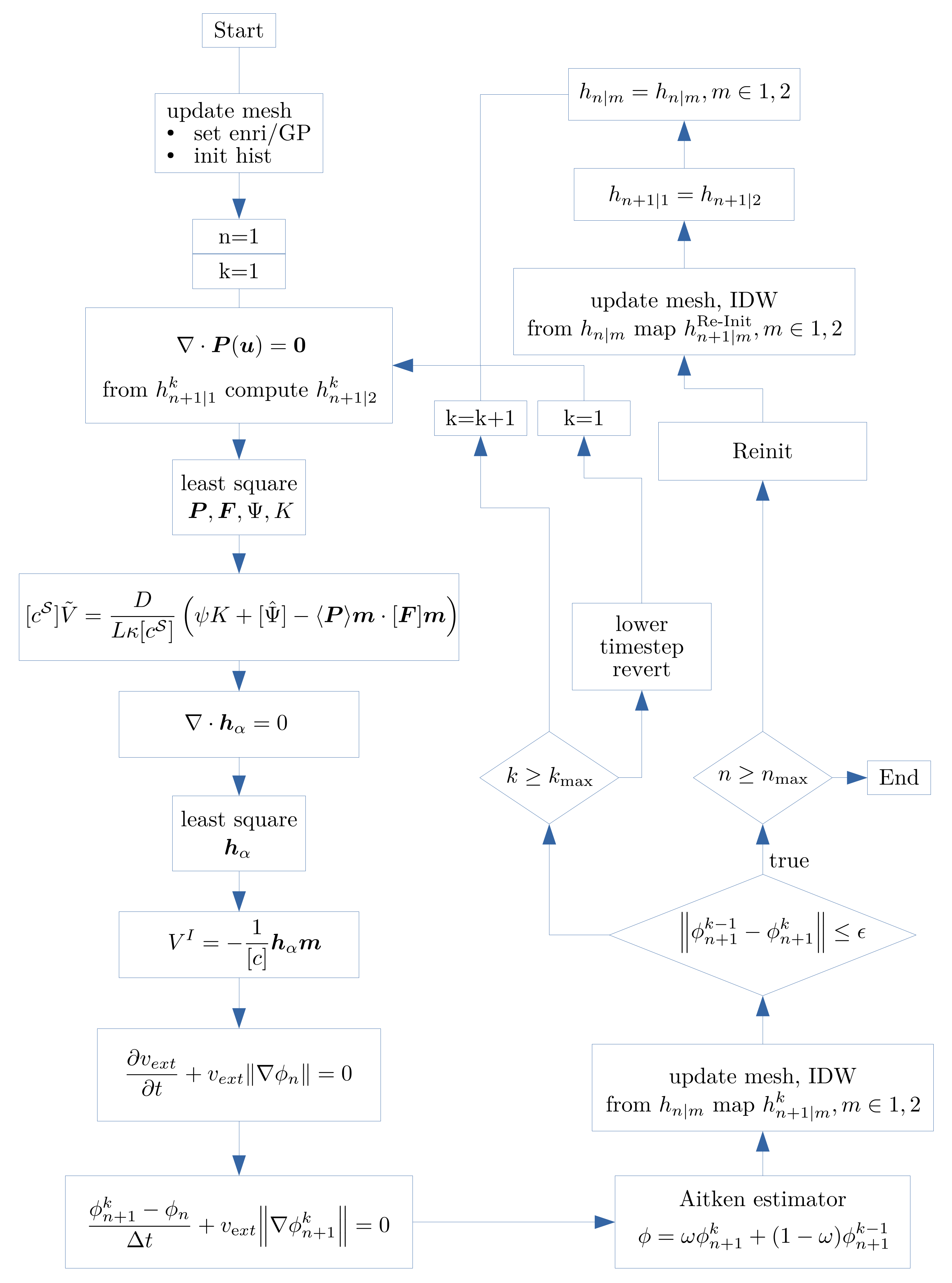
4.6. Staggered Solution Scheme

All partial differential equations are solved within the finite element method. Classically, XFEM-models for crack propagation employ a semi-explicit time integration scheme. In the first step, the mechanical fields are computed, which is followed by propagating the crack in a level set update that completes the timestep. In the current context, this is not suitable, since the explicit surface develops spatial and temporal surface instabilities. This can be attributed to the circumstance that, after such an explicit timestep, the updated geometry of the discontinuity does not exactly fulfill equilibrium. The interface may have traveled too far, which would lead to the reverse effect in the following timestep. This phenomenon can be mitigated by a fully implicit staggered approach, which has been adopted from [30].

The equations are iterated until the increment in $\varphi$ from one staggered iteration to the following decreases below a threshold. In order to speed up convergence, an Aitken ${\mathrm{\Delta }}^2$ method is employed to dampen the level set increment.

As the location of integration points is modified in each staggered iteration, material history needs to be transferred from the old to the new locations. This is accomplished using an inverse distance mapping procedure

$$f\left(\mathit{X}\right) = \frac{1}{{\sum }_i^n{w}_i\left(\mathit{X}\right)}\sum _i^n{w}_i\left(\mathit{X}\right)f_i,$$

(33)

where f is the smoothed quantity and the weights are defined by

$$w_i\left(\mathit{X}\right) = \frac{1}{{\Vert \mathit{X} - {\mathit{X}}_i\Vert }^2}.$$

(34)

Plastic deformation must not diffuse through the interface from the ductile matrix into the precipitate, as otherwise the stress- and deformation-state at the interface would be unphysical. Nevertheless, if the interface sweeps a volume, the volume should inherit the plastic deformation which was present at that location previously. Therefore, the old integration point may only contribute to the value of a new integration point scheme if:

• The old point is on the same side of the interface as the new point.
• The side is determined by the sign of the updated new level set.

A flow chart of the numerical procedure is depicted in Figure 2. More detailed information, e.g., sub-integration, is provided in [14].

5. Numerical Results

In this section, a number of simulations demonstrate the versatility of the method. An equilibrium shape is reproduced for model verification, the linear growth relation during Ostwald ripening is confirmed, and it is shown that plasticity qualitatively alters precipitate shapes.

5.1. Elastic Matrix

As a benchmark example, an equilibrium shape is recovered from an initially spherical precipitate with radius $r = 500\mathrm{nm}$ at the center of a cube with an edge length of $2000\mathrm{nm}$. The three symmetry boundary conditions for the balance of linear momentum are

• $X = 0$ with $u = 0$,
• $Y = 0$ with $v = 0$,
• $Z = 0$ with $w = 0$

with the components $u,v,w$ of the displacement field $\mathit{u}$. In order to obtain equilibrium shapes, no further mechanical boundary conditions are applied. The diffusion problem is only constrained by the immersed Dirichlet boundary within the domain. The zero-flux Neumann conditions on the surface of the computational domain preserve the volume of the inclusion, since no material is transported into the domain. All necessary material parameters are provided in

Table 2. Material parameters.

Elastic $\mathit{\gamma }$	and ${\mathit{\gamma }}^{\prime }$	Transformation $\mathit{\gamma }$	and ${\mathit{\gamma }}^{\prime }$
$C_{11}$	$215 \mathrm{GPa}$	D	$1.125·{10}^{ - 17} {\mathrm{m}}^2/\mathrm{s}$
$C_{12}$	$162 \mathrm{GPa}$	$\kappa$	$1.0417·{10}^9 \mathrm{J}/{\mathrm{m}}^3$
$C_{44}$	$77.6 \mathrm{GPa}$	$c_{\gamma }^{\mathcal{S}}$	$0.13$
$\delta$	$0.1\%$	$c_{{\gamma }^{\prime }}^{\mathcal{S}}$	$\frac{1}{1 + 3} = 0.25$
		L	$500 \mathrm{nm}$
		$\sigma$	$0.025 \mathrm{J}{\mathrm{m}}^2$

.

The equilibrium state (see Figure 3) is accepted if the conversion rate

$$k_{\mathrm{abs}} = {\int }_I\left|V_i^I\right|\mathrm{d}A$$

(35)

is reduced to 10% of its initial value. The expected cuboidal shape is recovered.

5.2. Ostwald Ripening

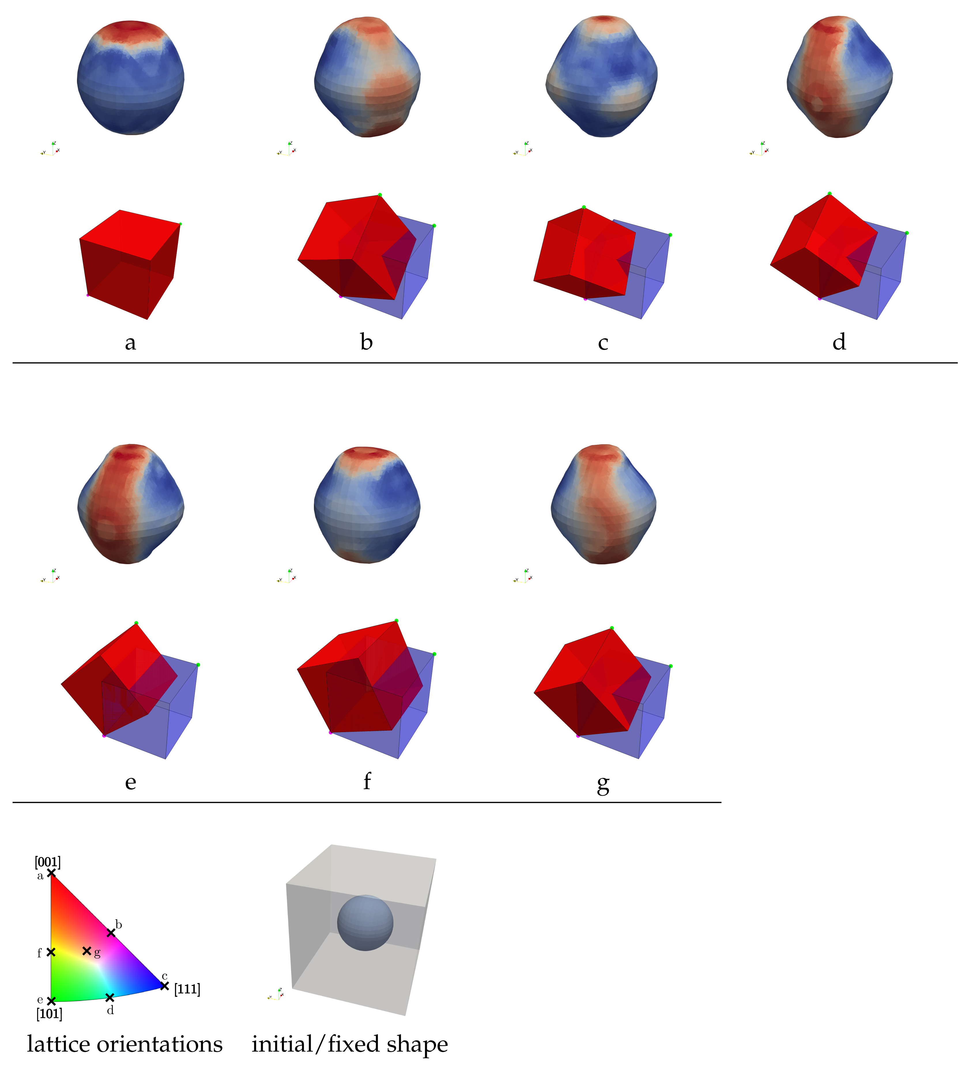
The main advantage of the diffusive model, however, does not lie in the possibility to recover equilibrium shapes. The diffusive model captures the flow of atoms in multi-particle systems. Large particles will grow in size at the expense of small particles, which is referred to as Ostwald ripening. This phenomenon is attributed to the elevated solute concentration on the surface of the small particles. A multi-particle problem was set up with particles of different radii. The boundary conditions are the same as for the previous example. It is observed that each particle on its own tends to its cuboidal equilibrium shape. Hence, initially most transport occurs close to the surface of the particle. However, diffusion also transports the solute atoms from the small towards the bigger particles. This is illustrated by streamlines of the concentration gradient field; see Figure 4. The particle growth and shrinkage are shown in Figure 5.

The theory by Lifshitz et al. [31] predicts a linear relationship of time to precipitate volume. The relationship is confirmed by tracking the volumes of a larger and a smaller particle in a two-precipitate simulation. The volumes of both precipitates are normalized with respect to their initial volumes. Linear growth and shrinkage can be observed, while the total volume remains approximately constant. The slight deviation in total volume underlines that the numerical procedure required to compute the normal fluxes of solute atoms is not mass preserving. The geometry and time evolution are provided in Figure 6.

5.3. Ductile Matrix

Plasticity has been identified as a key driver of the phase transformation. This can be attributed to the qualitatively changed stress and deformation state which enters the Gibbs–Thomson Equation (6).

The following simulation is based on the initial geometry of the Ostwald ripening case; see Figure 5. A displacement boundary condition is added at $Z = 2000\mathrm{nm}$ with $w = 0.015\mathrm{nm}$ over a timespan of $55.5\mathrm{h}$. The resulting tensile stress state activates plasticity, which modifies the precipitate shape. The interfacial velocity $V^I$ and the forest dislocation density ${\rho }_{\mathrm{F}}$ in the bulk are depicted in Figure 7.

In polycrystalline superalloys, each grain is oriented differently with respect to the load axis. However, it is well established that single crystals exhibit strong ductile anisotropy; see [32] or [33]. Hence, each grain will, by itself, show anisotropic creep rates.

In order to study the anisotropy, seven simulations were performed on a mesh of 30 finite elements in each direction. Each of the simulations was assigned a different but uniform lattice orientation. In conjunction with zero flux of solute atoms over the domain boundary, two sets of boundary conditions for the mechanical problem were applied. The first set contains the same boundary conditions as the previous example. The second set reads:

• $Z = 0$ with $w = 0$ (base symmetry plane).
• $Z = 0$ and $Y = 0$ with $v = 0$ (x-axis fixed in y-direction).
• $Z = 0$ and $X = 0$ with $u = 0$ (y-axis fixed in x-direction).

The specified orientations and resulting precipitate shapes for the second set of boundary conditions are provided in Figure 8. The load displacement curves of the fully diffusive model show only minor deviations from a simulation with a fixed interface; see Figure 9. It is, therefore, concluded that Schmid factors and boundary conditions play a more important role than an evolving precipitate geometry that remains a single particle. Nevertheless, the authors hypothesize that the mechanical response of the simulations with shape evolution will show larger deviations from the simulations with fixed interfaces if

• The precipitate volume fraction is increased.
• The phase transformation leads to changes in topology.

However, simulations meeting these points require handling of boundary conditions for the explicit surface, which will have to be addressed in future studies.

6. Conclusions and Outlook

A 3D SI model was presented and verified in a range of different initial and boundary conditions. The following results were reported:

• A SI model for phase transformations was extended by a path-dependent non-linear crystal plasticity model.
• The model captures cuboidal equilibrium shapes and Ostwald ripening.
• By solving the diffusion equation explicitly, the transport of solute atoms within the $\gamma$-matrix can be visualized.
• By introducing a crystal plasticity model the precipitate’s shape is qualitatively altered due to the anisotropy of the material’s mechanical response.
• For isolated precipitates, the shape changes do not influence the global mechanical behaviour, as was confirmed by simulations with a fixed interface.

Future research should aim at improving the maximum resolution with more efficient search algorithms and parallelism. This will allow an increase in the number of precipitates. Furthermore, the method should be extended by boundary conditions such that precipitates may intersect the domain boundary. Both enhancements will significantly enhance the applicability of the model to more realistic precipitate geometries.

References

1. Matan, N.; Cox, D.; Carter, P.; Rist, M.; Rae, C.; Reed, R. Creep of cmsx-4 superalloy single crystals: Effects of misorientation and temperature. Acta Mater. 1999, 47, 1549–1563. Available online: http://www.sciencedirect.com/science/article/pii/S1359645499000294 (accessed on 2 April 2022). [CrossRef]
2. McLean, M. The contribution of friction stress to the creep behaviour of the nickel-base in situ composite, γγ’-cr3c2. Proc. R. Soc. Lond. A. Math. Phys. Sci. 1980, 373, 93–109. [Google Scholar]
3. Dyson, B.F. Microstructure based creep constitutive model for precipitation strengthened alloys: Theory and application. Mater. Sci. Technol. 2009, 25, 213–220. [Google Scholar] [CrossRef]
4. Zhu, Z.; Basoalto, H.; Warnken, N.; Reed, R. A model for the creep deformation behaviour of nickel-based single crystal superalloys. Acta Mater. 2012, 60, 4888–4900. Available online: http://www.sciencedirect.com/science/article/pii/S1359645412003333 (accessed on 2 April 2022). [CrossRef]
5. Shenoy, M.; Tjiptowidjojo, Y.; McDowell, D. Microstructure-sensitive modeling of polycrystalline {IN} 100. Int. J. Plast. 2008, 24, 1694–1730. Available online: http://www.sciencedirect.com/science/article/pii/S0749641908000120 (accessed on 2 April 2022). [CrossRef]
6. le Graverend, J.-B.; Cormier, J.; Gallerneau, F.; Villechaise, P.; Kruch, S.; Mendez, J. A microstructure-sensitive constitutive modeling of the inelastic behavior of single crystal nickel-based superalloys at very high temperature. Int. J. Plast. 2014, 59, 55–83. Available online: http://www.sciencedirect.com/science/article/pii/S0749641914000473 (accessed on 2 April 2022). [CrossRef]
7. Zhou, J.; He, Y.; Shen, J.; Essa, F.A.; Yu, J. Ni/Ni3Al interface-dominated nanoindentation deformation and pop-in events. Nanotechnology 2021, 33, 105703. Available online: https://iopscience.iop.org/article/10.1088/1361-6528/ac3d62 (accessed on 2 April 2022). [CrossRef]
8. Zhao, Y. Stability of phase boundary between L12-Ni3Al phases: A phase field study. Intermetallics 2022, 144, 107528. [Google Scholar] [CrossRef]
9. Jokisaari, A.M.; Naghavi, S.S.; Wolverton, C.; Voorhees, P.W.; Heinonen, O.G. Predicting the morphologies of γ precipitates in cobalt-based superalloys. Acta Mater. 2017, 141, 273–284. [Google Scholar] [CrossRef]
10. Tsukada, Y.; Koyama, T.; Kubota, F.; Murata, Y.; Kondo, Y. Phase-field simulation of rafting kinetics in a nickel-based single crystal superalloy. Intermetallics 2017, 85, 187–196. Available online: http://www.sciencedirect.com/science/article/pii/S0966979516305337 (accessed on 2 April 2022). [CrossRef]
11. Ali, M.A.; Amin, W.; Shchyglo, O.; Steinbach, I. 45-degree rafting in ni-based superalloys: A combined phase-field and strain gradient crystal plasticity study. Int. J. Plast. 2020, 128, 102659. [Google Scholar] [CrossRef]
12. Schmidt, I.; Gross, D. The equilibrium shape of an elastically inhomogeneous inclusion. J. Mech. Phys. Solids 1997, 45, 1521–1549. Available online: http://www.sciencedirect.com/science/article/pii/S0022509697000112 (accessed on 2 April 2022). [CrossRef]
13. Zhao, X.; Duddu, R.; Bordas, S.; Qu, J. Effects of elastic strain energy and interfacial stress on the equilibrium morphology of misfit particles in heterogeneous solids. J. Mech. Phys. Solids 2013, 61, 1433–1445. [Google Scholar] [CrossRef]
14. Munk, L.; Reschka, S.; Loehnert, S.; Maier, H.J.; Wriggers, P. A sharp-interface model for diffusional evolution of precipitates in visco-plastic materials. Comput. Methods Appl. Mech. Eng. 2021, in press. [Google Scholar] [CrossRef]
15. Gurtin, M.E. Configurational Forces as Basic Concepts of Continuum Physics; Springer Science & Business Media: Berlin, Germany, 1999; Volume 137. [Google Scholar]
16. Fried, E.; Gurtin, M.E. Coherent solid-state phase transitions with atomic diffusion: A thermomechanical treatment. J. Stat. Phys. 1999, 95, 1361–1427. [Google Scholar] [CrossRef]
17. Leo, P.; Sekerka, R. Overview no. 86: The effect of surface stress on crystal-melt and crystal-crystal equilibrium. Acta Metall. 1989, 37, 3119–3138. [Google Scholar] [CrossRef]
18. Roters, F.; Eisenlohr, P.; Hantcherli, L.; Tjahjanto, D.; Bieler, T.; Raabe, D. Overview of constitutive laws, kinematics, homogenization and multiscale methods in crystal plasticity finite-element modeling: Theory, experiments, applications. Acta Mater. 2010, 58, 1152–1211. Available online: http://www.sciencedirect.com/science/article/pii/S1359645409007617 (accessed on 2 April 2022). [CrossRef]
19. Knowles, D.; Gunturi, S. The role of < 112>{111} slip in the asymmetric nature of creep of single crystal superalloy cmsx-4. Mater. Sci. Eng. A 2002, 328, 223–237. [Google Scholar]
20. Sass, V.; Glatzel, U.; Feller-Kniepmeier, M. Anisotropic creep properties of the nickel-base superalloy cmsx-4. Acta Mater. 1996, 44, 1967–1977. [Google Scholar] [CrossRef]
21. Voskoboinikov, R. Effective γ-surfaces in {111} plane in fcc ni and l1 2 ni 3 al intermetallic compound. Phys. Met. Metallogr. 2013, 114, 545–552. [Google Scholar] [CrossRef]
22. Fedorov, F.I. Theory of Elastic Waves in Crystals; Springer Science & Business Media: Berlin, Germany, 2013. [Google Scholar]
23. Wiedersich, H. Hardening mechanisms and the theory of deformation. JOM 1964, 16, 425–430. [Google Scholar] [CrossRef]
24. Belytschko, T.; Black, T. Elastic crack growth in finite elements with minimal remeshing. Int. J. Numer. Methods Eng. 1999, 45, 601–620. [Google Scholar] [CrossRef]
25. Moës, N.; Cloirec, M.; Cartraud, P.; Remacle, J.-F. A computational approach to handle complex microstructure geometries. Comput. Methods Appl. Mech. Eng. 2003, 192, 3163–3177. [Google Scholar] [CrossRef]
26. Babuška, I.; Banerjee, U. Stable generalized finite element method (sgfem). Comput. Methods Appl. Mech. Eng. 2012, 201, 91–111. [Google Scholar] [CrossRef]
27. Lekien, F.; Marsden, J. Tricubic interpolation in three dimensions. Int. J. Numer. Methods Eng. 2005, 63, 455–471. [Google Scholar] [CrossRef]
28. Osher, S.; Sethian, J.A. Fronts propagating with curvature-dependent speed: Algorithms based on hamilton-jacobi formulations. J. Comput. Phys. 1988, 79, 12–49. Available online: http://www.sciencedirect.com/science/article/pii/0021999188900022 (accessed on 2 April 2022). [CrossRef]
29. Brooks, A.N.; Hughes, T.J. Streamline upwind Petrov-Galerkin formulations for convection dominated flows with particular emphasis on the incompressible Navier-Stokes equations. Comput. Methods Appl. Mech. Eng. 1982, 32, 199–259. [Google Scholar] [CrossRef]
30. Sauerland, H.; Fries, T.-P. The extended finite element method for two-phase and free-surface flows: A systematic study. J. Comput. Phys. 2011, 230, 3369–3390. [Google Scholar] [CrossRef]
31. Lifshitz, I.M.; Slyozov, V.V. The kinetics of precipitation from supersaturated solid solutions. J. Phys. Chem. Solids 1961, 19, 35–50. [Google Scholar] [CrossRef]
32. Nitz, A.; Lagerpusch, U.; Nembach, E. CRSS anisotropy and tension/compression asymmetry of a commercial superalloy. Acta Mater. 1998, 46, 4769–4779. [Google Scholar] [CrossRef]
33. Jacome, L.A.; Nörtershäuser, P.; Heyer, J.-K.; Lahni, A.; Frenzel, J.; Dlouhy, A.; Somsen, C.; Eggeler, G. High-temperature and low-stress creep anisotropy of single-crystal superalloys. Acta Mater. 2013, 61, 2926–2943. [Google Scholar] [CrossRef]
Figure 1. Spherical inclusion commencing transformation into cuboid. Concentration gradient which is proportional to the material flux. Normalized interfacial concentration as a result of the stress-modified Gibbs–Thomson equation.
Metals 12 01261 g001
Figure 2. Flow chart of the numerical scheme. h n , m k are history data, where n is the time step; m   =   1 are the history data from the previous time step, but in the current mesh, m   =   2 are the history data in the current time step and k is the global staggered iteration counter.
Metals 12 01261 g002
Figure 3. Cuboidal equilibrium shape.
Metals 12 01261 g003
Figure 4. Flow of solute atoms during Ostwald ripening. The streamlines reveal which location on a surface element of a small particle deposits solute atoms to another surface element of a bigger particle.
Metals 12 01261 g004
Figure 5. Ostwald ripening of initially spherical particles of different radii.
Metals 12 01261 g005
Figure 6. Precipitate volumes during Ostwald ripening.
Metals 12 01261 g006
Figure 7. Plastic deformation visible by increased dislocation density ρ F modifies precipitate shape. Evaluated with Diffusion coefficient D   =   7.5 · 10     17 m 2 / s .
Metals 12 01261 g007
Figure 8. Final shapes of precipitates at tensile strain of 1 % after 17 h at different lattice orientations identified by letters (ag). Surface colour illustrates normal velocity (blue—negative, red—positive).
Metals 12 01261 g008
Figure 9. Load displacement curves of fully diffusive (black) vs. fixed (thick, coloured) precipitate model for orientations depicted in Figure 8 for two boundary condition setups.
Metals 12 01261 g009