Analysis of Hydrogen-Assisted Brittle Fracture Using Phase-Field Damage Modelling Considering Hydrogen Enhanced Decohesion Mechanism

Abstract

This study proposes a hydrogen-assisted fracture analysis methodology considering associated deformation and hydrogen transport inside a phase-field-based formulation. First, the hydrogen transport around a crack tip is calculated, and then the effect of hydrogen enhanced decohesion (HEDE) is modeled by defining the critical energy release rate as a function of hydrogen concentration. The proposed method is based on a coupled hydrogen mechanical damage under phase-field and implemented through a user subroutine in ABAQUS software. The test using compact tension (CT) sample is investigated numerically to study the hydrogen embrittlement on 45CrNiMoVA steel. Experimentally, the microstructural fracture presents a mixed brittle fracture mode, consisting of quasi-cleavage (QC) and intergranular (IG) fracture with hydrogen. This fracture mode is consistent with the suggested HEDE mechanism in the model. The simulation results show that hydrogen accumulates at the crack tip where positive hydrostatic stress is located. Moreover, the model estimates the initial hydrogen concentration through iterations. The simulated load-line displacement curves show good agreement with the experimental plots, demonstrating the predictive capabilities of the presented scheme.

1. Introduction

During the material forming processes, the atomic hydrogen tries to penetrate the metal and causes degradation of mechanical properties. Due to the degradation of mechanical properties, the metal may lose its strength and ductility, and an embrittlement fracture will occur. This phenomenon is called hydrogen embrittlement (HE). According to reported studies, Johnson [1] was the first who observed the phenomenon of hydrogen embrittlement in steel in 1875 and concluded that hydrogen may lead to significant deterioration of mechanical properties of steel and could produce brittle fracture without warning. Since then, the hydrogen-assisted fracture properties of the metals have attracted much attention. The related experimental research shows that the fracture micro-mechanisms transformed from dimples ductile fracture (microvoid coalescence (MVC)) without hydrogen to brittle fracture (quasi-cleavage (QC) or intergranular (IG) fracture + transgranular (TG) fracture mechanism) with hydrogen [2,3]. For various hydrogen-induced cracking phenomena, there is no unified theory that explains the mechanism underlying HE. To date, there are two generally accepted HE mechanisms: hydrogen-enhanced localized plasticity (HELP) and hydrogen-enhanced decohesion (HEDE). Birnbaum et al. [4], Sofronis et al. [5], and Liang et al. [6] introduced the HELP mechanism, which was subsequently applied to the unit cell model by Ahn et al. [7] to explore the influence of HELP on void expansion and coalescence. However, the HELP mechanism has no effect on the material’s yield strength. To fully characterize hydrogen embrittlement, it must be paired with other theories such as HEDE. At first, Pfeil [8] introduced the HEDE mechanism, which was further investigated by Troiano [9], Gerberich et al. [10], and Oriani [11]. The HEDE assumes that the presence of hydrogen in metal reduces the interatomic bonding force between adjacent crystallographic planes. During the fracture propagation, ductility tends to convert into brittleness when hydrogen concentration near the crack tip reaches a certain amount, lowering cohesive strength and surface energy along the grain boundary.

Experiments can be performed to determine the macroscopic characteristic curve and microscopic fracture mechanism of hydrogen embrittlement. A computational model can be developed by considering the hydrogen influence in the HEDE mechanism to predict hydrogen diffusion around a crack tip and to understand hydrogen embrittlement. Jiang and Carter [12] evaluated the fracture energy of iron that was degraded due to a hydrogen attack. They used the Born Haber thermodynamic cycle and discovered that the fracture energy reduces with an increasing hydrogen coverage. In another study, Serebrinsky [13] proposed a hydrogen degradation law based on decreasing the cohesive strength with increasing hydrogen concentration. Jembieet al. [14] and Sobhaniaragh et al. [15] simulated hydrogen-assisted fracture by using the cohesive zone model with the HEDE mechanism. Using a similar methodology, Li et al. [16] simulated hydrogen-assisted brittle fracture initiation in low alloy 30CrMo steel using the so-called three-step FE procedure coupled with hydrogen-informed CZM analysis for the HE problem. In recent studies, the phase-field model is employed by researchers to model brittle fractures. This model offers certain advantages, such as, it is easy to implement, capturing the original finite element model, and can mimic complex cracking processes (such as branching and merging of cracks). The Griffith theory [17] serves as the foundation for the phase-field model. Francfort et al. [18] used the quasi-static crack evolution of establishing the variational model that does not set a predefined crack path, hence bypassing the limitations of the Griffith theory. Bourdin et al. [19,20] investigated the viability of numerical approaches. They considered a diffuse crack region that was dominated by a phase-field variable to characterize the material’s sharp fracture surface topology, which was interpolated between intact and shattered materials. Miehe et al. [21,22] proposed an operator splitting approach that updates the crack phase and displacement fields progressively to predict brittle fracture. Miehe et al. [23] further developed the phase-field modeling of ductile fracture by including the plastic behavior. Ambati et al. [24,25] applied the follow-up model by integrating the degradation function and the plastic strain state to forecast crack initiation in the plastic zone. Their study compared the numerical results to experimental data. Based on the fracture criterion of the phase-field model and its advantages to simulate the fracture mechanism, many researchers have adopted this to simulate the phenomenon of HE. In this method, hydrogen diffusion and the subsequent fracture are studied within the framework of a phase-field model. Philip et al. [26] introduced hydrogen diffusion, plastic strain gradient, and the phase-field fracture formula relating the hydrogen sensitivity. The hydrogen sensitivity is calculated by the first principles into the framework of the phase-field model to predict hydrogen-assisted fracture. Martnez-Paeda et al. [27] presented the hydrogen-assisted cracking phase-field formula using the finite element approach (FEM). Additionally, Wu et al. [28] introduced the phase-field regularized cohesive model (PF-CZM) to simulate hydrogen-induced fractures.

The presented study proposes a hydrogen-assisted fracture phase-field model that incorporates the coupled problems of hydrogen transport and the HEDE mechanism to capture hydrogen’s effect on damage evolution. The remainder of the paper is structured in the following manner. Section 2 provides an overview of the phase-field model. Following that, the link between hydrogen transport and hydrogen-assisted deterioration is established. Section 3 explains the implementation of finite element analysis in ABAQUS via user subroutine UEL. Section 4 explains the hydrogen-charged (CT) specimens of 45CrNiMoVA steel to demonstrate the capability of the numerical model. This section also covers the analysis and discussion of simulation results. Finally, Section 5 draws important conclusions.

2. Hydrogen Assisted Fracture Theory Based on Phase-Field Model

2.1. Phase Field Approximation of Diffusive Crack Topology

Miehe et al. suggested the phase-field model of the diffusive crack [21,22,23]. The model was developed by considering an infinite one-directional bar having a constant cross-sectional area $\Gamma$ along the x-axis and occupying a solid body $\Omega$. Where $\Gamma$ denotes the completely fractured crack surface. The sharp crack topology can be characterized by a field variable $\varphi \left(x\right)\in \left[0,1\right]$. Where $\varphi =0$ represents the material in an entirely intact state and $\varphi =1$ represents the material in a completely broken state. Assuming the bar is completely open at $x=0$, the non-smooth crack topology can be modeled using the exponential function:

$$\varphi \left(x\right)=e^{-\frac{\left|x\right|}{l}}$$

(1)

where $l$ is a length scale parameter and $\varphi \left(x\right)$ is the phase-field value of the diffusive crack topology surface. By assuming that the length scale $l\to 0$, then sharp case is approached and Equation (1) decays monotonically to zero because of moving away from the crack location.

Equation (1) is the solution of the ordinary differential equation for $x\ne 0$ as follows:

$${\varphi }^{″}\left(x\right)-\frac{1}{l^2}\varphi \left(x\right)=0$$

(2)

Equation (2) follows the Dirichlet-type boundary conditions: $\varphi \left(0\right)=1$ and $\varphi \left(\pm \infty \right)=0$. This can be transformed into the Euler–Lagrange equation of the variational problem $\varphi =\arg \left\{\underset{\varphi \in W}{\inf }I\left(\varphi \right)\right\}$ with $W=\left\{\varphi |\varphi (0)=1,\varphi (\pm \infty )=0\right\}$. The associated quadratic functional is then given by:

$$I\left(\varphi \right)={\displaystyle {\int }_{-\infty }^{\infty }\frac{1}{2}}\left[{\varphi }^2+l^2{\left({\varphi }^{\prime }\right)}^2\right]\mathrm{d}x$$

(3)

The integration over the volume domain $\mathrm{d}\mathrm{V}=\Gamma \mathrm{d}x$ gives $I(\varphi =e^{-\left|x\right|/l})=l\Gamma$; therefore, the crack surface $\Gamma$ is related to the crack length scale parameter $l$. Consider a discrete internal discontinuity $\Gamma$ in a solid body $\Omega$, the crack surface density ${\Gamma }_l\left(\varphi \right)$ is introduced by means of the regularized crack functional as:

$${\Gamma }_l\left(\varphi \right)=\frac{1}{l}I\left(\varphi \right)={\displaystyle {\int }_{\Omega }\frac{1}{2l}\left({\varphi }^2+l^2{\left({\varphi }^{\prime }\right)}^2\right)\mathrm{d}\mathrm{V}}={\displaystyle {\int }_{\Omega }{r}_l\left(\varphi ,{\varphi }^{\prime }\right)}\mathrm{d}\mathrm{V}$$

(4)

where $r_l\left(\varphi ,{\varphi }^{\prime }\right)$ denotes the one-dimensional crack surface density function. Similarly, it can be stated as follows in higher dimensions:

$$r_l\left(\varphi ,\nabla \varphi \right)=\frac{1}{2l}{\varphi }^2+\frac{l}{2}{\left|\nabla \varphi \right|}^2$$

(5)

where $\nabla \varphi$ represents the spatial gradient of $\varphi$.

The fracture energy dissipated by the formation of a crack can be calculated as [29]:

$${\displaystyle \underset{\Gamma }{\int }{G}_{\mathrm{c}}\mathrm{d}\Gamma }\approx {\displaystyle \underset{\Omega }{\int }{G}_{\mathrm{c}}}{\gamma }_l\left(\varphi ,\nabla \varphi \right)\mathrm{d}\mathrm{V}={\displaystyle \underset{\Omega }{\int }{G}_{\mathrm{c}}}\left(\frac{1}{2l}{\varphi }^2+\frac{l}{2}{\left|\nabla \varphi \right|}^2\right)\mathrm{d}\mathrm{V}$$

(6)

where $G_c$ is the critical energy release rate.

The total potential energy of a solid body can be used to relate the bulk energy ${\Psi }^b\left(\mathbf{u},\varphi \right)$ to the fracture energy ${\Psi }^s\left(\varphi \right)$ as [29]:

$$\Psi \left(\mathbf{u},\varphi \right)={\Psi }^b\left(\mathbf{u},\varphi \right)+{\Psi }^s\left(\varphi \right)={\displaystyle \underset{\Omega }{\int }\left\{{\left(1-\varphi \right)}^2{\psi }_0\left(\mathsf{\epsilon }\right)+{\displaystyle \underset{\Omega }{\int }{G}_c}\left(\frac{1}{2l}{\varphi }^2+\frac{l}{2}{\left|\nabla \varphi \right|}^2\right)\right\}}\mathrm{d}\mathrm{V}$$

(7)

where $\mathbf{u}$ is the vector of displacements and ${\psi }_0\left(\mathsf{\epsilon }\right)$ is the elastic strain energy density, is defined as a function of the standard strain tensor $\mathsf{\epsilon }$ and the fourth-order linear elastic tensor ${\mathbf{C}}_0$. This can be expressed as [30]:

$${\psi }_0\left(\mathsf{\epsilon }\right)=\frac{1}{2}{\mathsf{\epsilon }}^T:{\mathbf{C}}_0:\mathsf{\epsilon }$$

(8)

Such that, assuming a small strain theory, the standard strain tensor $\mathsf{\epsilon }$ can be calculated as: $\mathsf{\epsilon }=\frac{1}{2}\left[{\left(\nabla \mathbf{u}\right)}^T+\nabla \mathbf{u}\right]$.

2.2. Governing Balance Equations

By taking the variation of the total potential energy (Equation (7)) can be written (weak form) with respect to $\mathsf{\epsilon }$ and $\varphi$ renders in the absence of body forces and external tractions, which can be expressed as:

$${\displaystyle {\int }_{\Omega }\left\{\mathsf{\sigma }:\delta \mathsf{\epsilon }-2\left(1-\varphi \right)\delta \varphi {\psi }_0\left(\mathsf{\epsilon }\right)+G_c\left[\frac{1}{l}\varphi \delta \varphi +l\nabla \varphi \cdot \nabla \delta \varphi \right]\right\}\mathrm{d}\mathrm{V}}=0$$

(9)

where the Cauchy stress tensor is expressed as: $\mathsf{\sigma }=\frac{\partial {\psi }_0\left(\mathsf{\epsilon }\right)}{\partial \mathsf{\epsilon }}=g\left(\varphi \right){\mathsf{\sigma }}_0={\left(1-\varphi \right)}^2{\mathbf{C}}_0:\mathsf{\epsilon }$.

Application of the Gauss theorem, the corresponding Eulerian equations can be written (strong form) for or any arbitrary value of the kinematic variables $\delta \mathbf{u}$ and $\delta \varphi$:

$$\begin{gathered} \nabla \cdot \mathsf{\sigma }=0 \\ {G}_c\left(\frac{1}{l}\varphi -l\Delta \varphi \right)-2\left(1-\varphi \right){\psi }_0\left(\mathsf{\epsilon }\right)=0 \end{gathered}$$

(10)

To ensure the irreversibility when the elastomer is pressed or unloaded, the so-called history variable field H can be explained as [31]:

$$H=\{\begin{array}{cc}{\psi }_0\left(\mathsf{\epsilon }\right)& {\psi }_0\left(\mathsf{\epsilon }\right)>H_t\\ H_t& otherwise\end{array}$$

(11)

where $H_t$ is the energy determined at any specific time increment t.

Equations (10) and (11) can be combined to obtain the phase-field damage evolution equation which satisfies the Kuhn–Tucker conditions:

$$G_c\left(\frac{1}{l}\varphi -l\Delta \varphi \right)-2\left(1-\varphi \right)H=0$$

(12)

2.3. Governing Equation of Hydrogen Diffusion

The hydrogen diffusion analysis under conditions of stress is defined as an extension of Fick’s law [32]. The diffusion equation is developed by using the law of mass conservation for diffusion:

$${\displaystyle \underset{\Omega }{\int }\frac{\mathrm{d}C}{\mathrm{d}t}}\mathrm{d}\mathrm{V}+{\displaystyle \underset{\partial \Omega }{\int }\mathit{J}}\cdot \mathit{n}\mathrm{d}S=0$$

(13)

where $C$ is the diffusible hydrogen concentration in a solid body $\Omega$, $\mathit{J}$ is the hydrogen flux and $\mathit{n}$ is the outward unit vector normal to the surface $\partial \Omega$.

The strong form of the balanced equation can be obtained by using the divergence theorem for any arbitrary volume:

$$\frac{\mathrm{d}C}{\mathrm{d}t}+\nabla \cdot \mathit{J}=0$$

(14)

For an arbitrary, suitably continuous, scalar field, $\mathsf{\delta }C$, the variational statement Equation (14) can be written as:

$${\displaystyle \underset{\Omega }{\int }\mathsf{\delta }C}\left(\frac{\mathrm{d}C}{\mathrm{d}t}+\nabla \cdot \mathit{J}\right)\mathrm{d}\mathrm{V}=0$$

(15)

Again, using the divergence theorem, the weak form of the equilibrium equation can be expressed as:

$${\displaystyle \underset{\Omega }{\int }\left[\mathsf{\delta }C\left(\frac{\mathrm{d}C}{\mathrm{d}t}\right)-\mathit{J}\cdot \nabla \mathsf{\delta }C\right]\mathrm{d}\mathrm{V}+{\displaystyle \underset{\partial \Omega }{\int }q\mathsf{\delta }C}}\mathrm{d}\mathrm{S}=0$$

(16)

where $q=\mathit{J}\cdot \mathit{n}$ is the concentration flux exiting the body across $\partial \Omega$.

The chemical potential $\mu$ gradient instigates the diffusion process, and it can be expressed as [29]:

$$\mu ={\mu }^0+RT\ln \frac{{\theta }_L}{1-{\theta }_L}-V_H{\sigma }_H$$

(17)

where ${\mu }^0$ is the chemical potential at a reference state, $V_H$ is the partial molar volume of hydrogen ($2000 {\mathrm{mm}}^3/\mathrm{mol}$ for iron [33]), $T$ is the temperature, $R$ is the ideal constant of gas ($8314 \mathrm{N}\cdot \mathrm{mm}/\mathrm{mol}\cdot \mathrm{K}$), ${\theta }_L$ is the occupancy of the lattice sites, and ${\sigma }_H$ is the hydrostatic stress defined as by ${\sigma }_H=\left({\sigma }_{11}+{\sigma }_{22}+{\sigma }_{33}\right)/3$.

A linear Onsager relationship is used to relate the flow to the chemical potential:

$$\mathit{J}=-\frac{DC}{RT}\nabla \mu$$

(18)

where $D$ is the ideal diffusivity. By substituting Equation (17) into Equation (18), and assuming the low occupancy (${\theta }_L\ll 1$) for most practical purposes, the diffusion flux can be expressed as:

$$\mathit{J}=-D\nabla C+\frac{D}{RT}C{V}_H\nabla {\sigma }_H$$

(19)

Substituting Equation (19) into Equation (16), the hydrogen diffusion equation can be obtained as:

$${\displaystyle \underset{\Omega }{\int }\left[\mathsf{\delta }C\left(\frac{1}{D}\frac{\mathrm{d}C}{\mathrm{d}t}\right)+\nabla \mathsf{\delta }C\cdot \nabla C-\nabla \mathsf{\delta }C\cdot \left(\frac{C{V}_H}{RT}\nabla {\sigma }_H\right)\right]}\mathrm{d}\mathrm{V}=-\frac{1}{D}{\displaystyle \underset{\partial {\Omega }_q}{\int }q\mathsf{\delta }C\mathrm{d}\mathrm{S}}$$

(20)

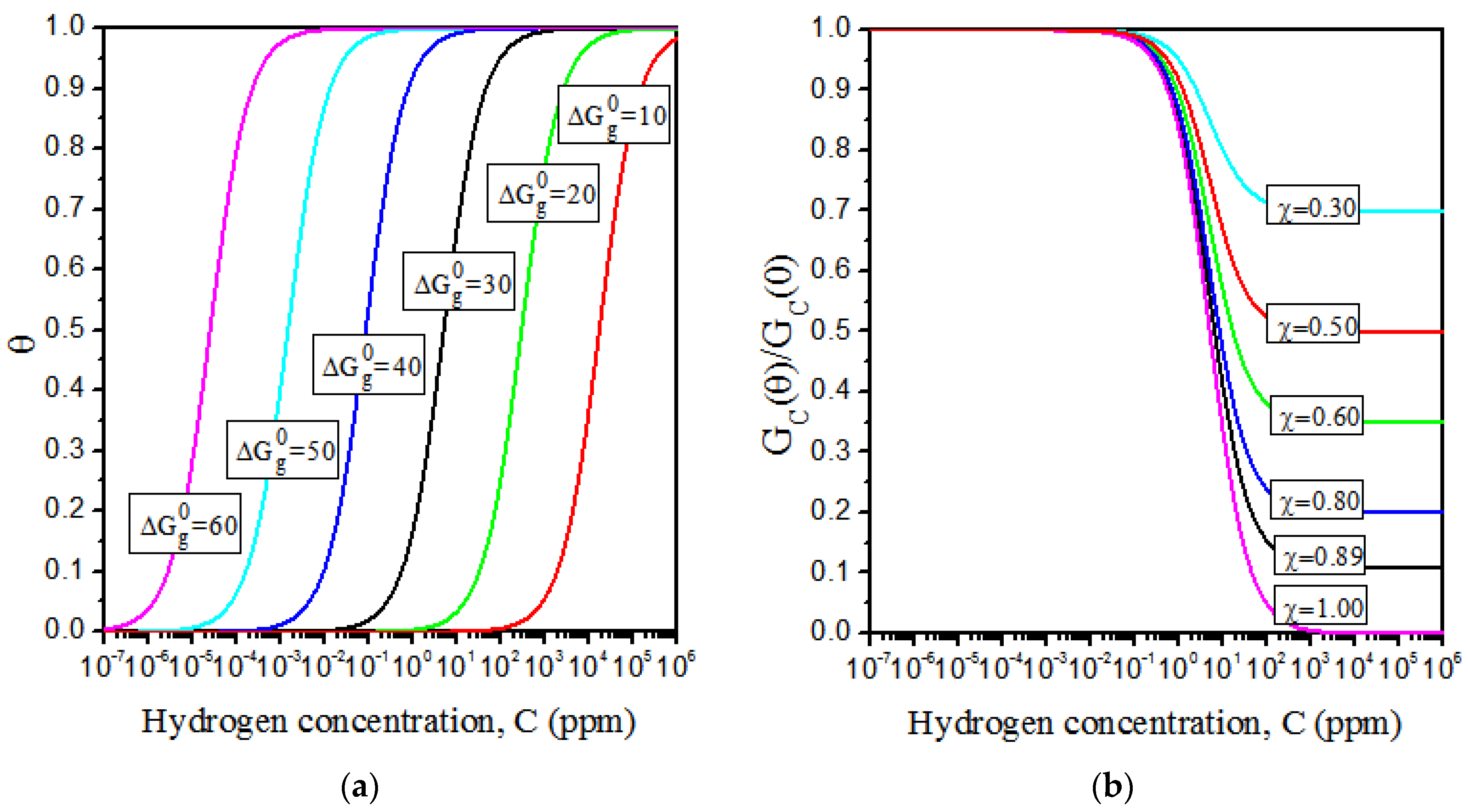
2.4. Hydrogen Degradation Function

Atomic hydrogen dissolved in metal reduces the binding energy between metal atoms and leads to a reduction in fracture resistance. Alvaro et al. [34] proposed a HEDE model in which the surface energy decreases linearly with an increase in hydrogen concentration. According to this model, a quantum-mechanically informed hydrogen-dependent degradation function can be defined as:

$$G_c\left(\theta \right)=\left(1-\chi \theta \right)G_c\left(0\right)$$

(21)

where $G_c\left(\theta \right)$ represents the critical energy release rate with the HEDE effect and χ denotes the hydrogen damage factor, $G_c\left(0\right)$ is the critical energy release rate with no hydrogen influence.

Considering the hydrogen coverage $\theta$ as a function of the bulk hydrogen concentration $C$ the framework of the Langmuir–McLean isotherm is defined as [12,35]:

$$\theta =\frac{C}{C+\exp (-\Delta G_g^0/RT)}$$

(22)

where $C$ is the impurity mole fraction in units and $\Delta G_g^0$ is the Gibbs free energy.

As defined in Equations (21) and (22), the hydrogen embrittlement parameter $G_C\left(\theta \right)/G_C\left(0\right)$ is dependent on the selected value of Gibbs free energy and hydrogen damage factor. The curves of hydrogen coverage with hydrogen concentration for various levels of Gibbs free energy range of 10 to 60 k/mol are shown in Figure 1a. Clearly, hydrogen concentration covers about four orders of magnitude for two parameters. The lower boundary and the upper boundary represent the hydrogen concentration at fracture initiation and the ultimate saturation level, respectively. Therefore, the value of the Gibbs free energy is very important and cannot be determined arbitrarily. The Gibbs free energy $\Delta G_g^0$ is assigned a value of 30 kJ/mol, representing the initiation hydrogen concentration and an ultimate saturation level ranging between 0.01 and 100 ppm in the α-Fe grain boundary [13].

The Gibbs free energy $\Delta G_g^0$ is fixed at a value of 30 kJ/mol. The curves of hydrogen embrittlement $G_C\left(\theta \right)/G_C\left(0\right)$ with hydrogen concentration for various levels of the hydrogen damage factor $\chi$ range of 0.30 to 1.00 are shown in Figure 1b. Considering the initiation hydrogen concentration ranging between 0.01 and 100 ppm, the hydrogen embrittlement parameter $G_C\left(\theta \right)/G_C\left(0\right)$ values decrease with the value of $\chi$ increasing. That is to say, the larger the $\chi$ value, the lower the critical energy release rate of hydrogen influence, and the hydrogen-induced fracture will easily occur. According to Jiang and Carter’s DFT (Periodic Density Functional) calculations [12], for iron, χ value is taken as 0.89.

3. Finite Element Implementation

To implement the solution in ABAQUS, the displacements, phase-field, and hydrogen concentration nodal values are interpolated using Voigt notation:

$$\mathbf{u}={\displaystyle \sum _{i=1}^m{\mathbf{N}}_i^{\mathbf{u}}{\mathbf{u}}_i}, \varphi ={\displaystyle \sum _{i=1}^m{N}_i}{\varphi }_i, C={\displaystyle \sum _{i=1}^m{N}_i}{C}_i$$

(23)

where $m$ denotes the number of nodes, and $N_i$ is the shape function associated with node $i$, ${\mathbf{u}}_i={\{u_x,u_y\}}^T$ is the displacement vector at the node $i$. The shape function matrix is expressed as: ${\mathbf{N}}_i^{\mathbf{u}}=\left[\begin{array}{cc}{N}_i& 0\\ 0& N_i\end{array}\right]$.

The gradient quantities associated with displacements, phase field, and hydrogen concentration are as follows:

$$\mathsf{\epsilon }={\displaystyle \sum _{i=1}^m{\mathbf{B}}_i^u}{\mathbf{u}}_i, \nabla \varphi ={\displaystyle \sum _{i=1}^m{\mathbf{B}}_i}{\varphi }_i, \nabla C={\displaystyle \sum _{i=1}^m{\mathbf{B}}_i{C}_i}$$

(24)

where ${\mathbf{B}}_i^u$ stands for the strain-displacement matrices and ${\mathbf{B}}_i$ represents the spatial derivatives of the shape functions, which can be described as follows:

$${\mathbf{B}}_i=\left[\begin{array}{c}{N}_{i,x}\\ N_{i,y}\end{array}\right], {\mathbf{B}}_i^{\mathbf{u}}=\left[\begin{array}{cc}{N}_{i,x}& 0\\ 0& N_{i,y}\\ N_{i,y}& N_{i,x}\end{array}\right]$$

(25)

where $N_{i,x}$ and $N_{i,y}$ are the derivatives of the corresponding shape function with respect to $x$ and $y$, respectively.

3.1. Finite Element Discretization of the Deformation Phase-Field

The residual vectors for the displacement and phase-fields can be considered that Equation (9) must hold for arbitrary values of $\mathsf{\delta }\mathbf{u}$ and $\mathsf{\delta }\varphi$, which can be expressed as [29]:

$${\mathbf{r}}_i^u={\displaystyle \underset{\Omega }{\int }\left\{\left[{\left(1-\varphi \right)}^2+k\right]{\left({\mathbf{B}}_i^u\right)}^T{\mathsf{\sigma }}_0\right\}}\mathrm{d}\mathrm{V}$$

(26)

$$r_i^{\varphi }={\displaystyle \underset{\Omega }{\int }\left[-2\left(1-\varphi \right)N_{i}H+G_C\left(\theta \right)\left(\frac{1}{l}{N}_i\varphi +l{\mathbf{B}}_i^T\nabla \varphi \right)\right]}\mathrm{d}\mathrm{V}$$

(27)

The value of the parameter k is set as the minimum to help in converging the solution. Normally, a value of k = 1 × 10⁻⁷ is used [31].

By differentiating the residuals for the incremental nodal variables, the components of the consistent stiffness matrices for the displacement field and phase field can be developed as:

$${\mathbf{K}}_{ij}^u=\frac{\partial {\mathbf{r}}_i^u}{\partial {\mathbf{u}}_j}={\displaystyle \underset{\Omega }{\int }\left\{\left[{\left(1-\varphi \right)}^2+k\right]{\left({\mathbf{B}}_i^u\right)}^T{\mathbf{C}}_{\mathrm{ep}}{\mathbf{B}}_j^u\right\}}\mathrm{d}\mathrm{V}$$

(28)

$${\mathbf{K}}_{ij}^{\varphi }=\frac{\partial r_i^{\varphi }}{\partial {\varphi }_j}={\displaystyle \underset{\Omega }{\int }\left[\left(2H+\frac{G_C\left(\theta \right)}{l}\right)N_i{N}_j+G_C\left(\theta \right)l{\mathbf{B}}_i^T{\mathbf{B}}_j\right]}\mathrm{d}\mathrm{V}$$

(29)

where ${\mathbf{C}}_{\mathrm{ep}}$ in Equation (28) is the linear elastic stiffness matrix.

Employing the Newton–Raphson method, the following equation can be solved iteratively [21]:

$${\left\{\begin{array}{c}\mathbf{u}\\ \varphi \end{array}\right\}}_{n+1}={\left\{\begin{array}{c}\mathbf{u}\\ \varphi \end{array}\right\}}_n-{\left[\begin{array}{cc}{\mathbf{K}}^{\mathbf{u}}& 0\\ 0& {\mathbf{K}}^{\varphi }\end{array}\right]}^{-1}{\left\{\begin{array}{c}{\mathbf{r}}^{\mathbf{u}}\\ r^{\varphi }\end{array}\right\}}_n$$

(30)

3.2. Finite Element Discretization of the Hydrogen Diffusion

Equation (20) can be discretized to generate the corresponding residual vector for any arbitrary virtual variation of the hydrogen concentration $\mathsf{\delta }C$:

$$r_i^C={\displaystyle \underset{\Omega }{\int }\left[N_i^T\left(\frac{1}{D}\frac{\mathrm{d}C}{\mathrm{d}t}\right)+{\mathbf{B}}_i^T\nabla C-{\mathbf{B}}_i^T\left(\frac{V_{H}C}{RT}\nabla {\sigma }_H\right)\right]}\mathrm{d}V$$

(31)

From which can be used to create a diffusivity matrix:

$${\mathbf{K}}_{ij}^C=\frac{\partial r_i^C}{\partial C_j}={\displaystyle \underset{\Omega }{\int }\left({\mathbf{B}}_i^T{\mathbf{B}}_j-{\mathbf{B}}_i^T\frac{V_H}{RT}\nabla {\sigma }_H{N}_j\right)}\mathrm{d}V$$

(32)

To solve the diffusion matrix, it is necessary to obtain the hydrostatic stress gradient $\nabla {\sigma }_H$, which is computed from integration points ${\sigma }_H$ values, extrapolated to the nodes using each element shape function, and subsequently multiplied by ${\mathbf{B}}_i$ to compute $\nabla {\sigma }_H$.

According to the standard finite element formulation using the Galerkin method, we can obtain the discretized hydrogen transport equation with an unknown vector for the hydrogen concentration $C$, as follows [36]:

$${\mathbf{K}}^{C}C+\mathbf{M}\dot{C}=\mathbf{F}$$

(33)

The concentration capacity matrix and the diffusion flux vector are given by:

$$\begin{array}{c}{\mathbf{M}}_{ij}={\displaystyle \underset{\Omega }{\int }{N}_i^T}\frac{1}{D}{N}_j\mathrm{d}\mathrm{V}\\ {\mathbf{F}}_i=-\frac{1}{D}{\displaystyle \underset{\partial {\Omega }_q}{\int }{N}_i^{T}q\mathrm{d}\mathrm{S}}\end{array}$$

(34)

where ${\mathbf{N}}_i$ is the shape function associated with node i, q the hydrogen flux vector on the surface with an outward normal unit vector $\mathit{J}\cdot \mathit{n}$.

We can perform the transient hydrogen diffusion analysis by solving Equation (33) by means of discretizing the time-derivative of $C$ using the backward Euler method.

3.3. Finite Element Implementation in ABAQUS

To solve the coupled mechanical diffusion phase field problem (Equations (30) and (33)), the finite element (FE) approach is implemented in ABAQUS via user subroutine UEL. The element’s characteristics include four integration points and isoparametric 2D quadrilateral quadratic with four degrees of freedom per node, namely $u_x$, $u_y$, $\varphi$ and C. In ABAQUS/VIEWER, the user element subroutine has the drawback that integration point variables cannot be visualized, considering this limitation, we adopted an auxiliary dummy mesh taking the same number of nodes at integration points that are used in the user-defined element, (i.e., CPE8R). A user material subroutine (UMAT) allows the user to create the constitutive matrix and estimate stresses from the strain data. In this auxiliary mesh, the stress components and the constitutive matrix are made equal to zero, (i.e., they have no influence on the solution of the global system). The corresponding material response is calculated at each integration point in the auxiliary mesh. The data from the developed user subroutine (UEL) is saved in a Fortran module and exported in the UMAT subroutine. The equivalence between model variables and SDVs (Solution-Dependent state variables) are shown in

Table 1. List of solution-dependent state variables in two-dimensional.

Variable	Number of SDV in ABAQUS
Axial stress—${\sigma }_{11}$, ${\sigma }_{22}$	SDV1, SDV2
Shear stress—${\sigma }_{12}$	SDV3
Axial strain—${\epsilon }_{11}$, ${\epsilon }_{22}$	SDV4, SDV5
Shear strain—${\epsilon }_{12}$	SDV6
Crack phase-field—$\varphi$	SDV7
Hydrostatic stress—${\sigma }_H$	SDV8
Hydrogen concentration—C	SDV9

.

4. Numerical Modeling

In Section, we have considered the compact tension CT specimens of 45CrNiMoVA steel that were hydrogen-charged to track the experimental load-displacement curves and characterize failure microstructural characteristics. Afterward, a hydrogen-assisted CT specimen failure model is developed to compare the simulation result with experimental data and to demonstrate the model’s predictive capability for hydrogen-assisted brittle fracture.

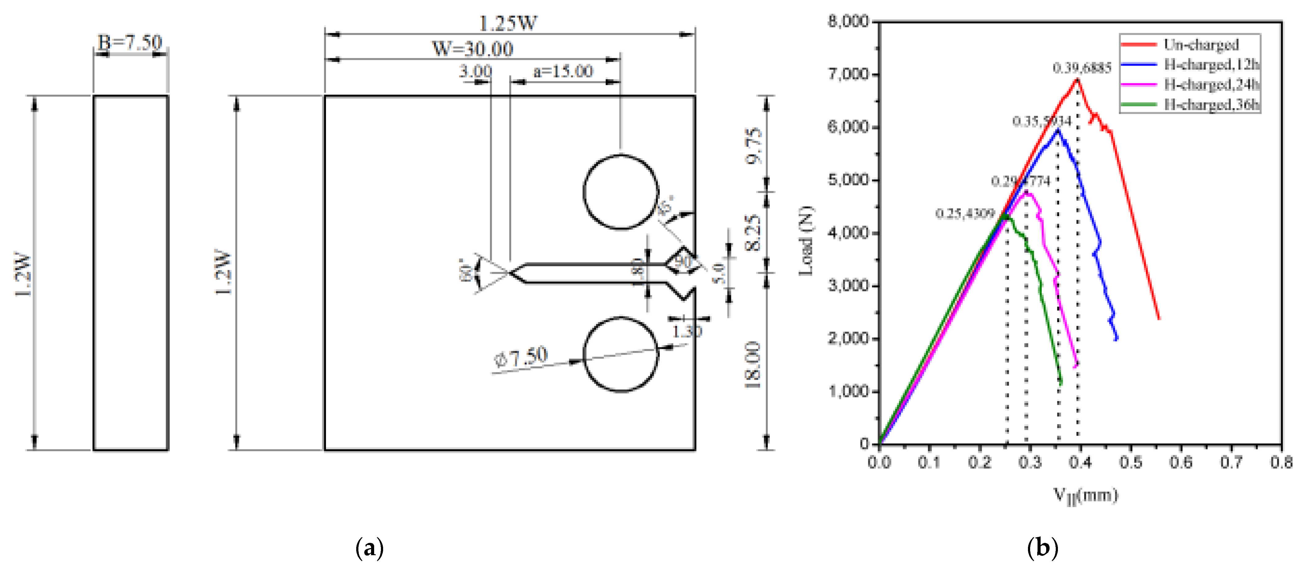
4.1. Material and Experiment

A round bar of 45CrNiMoVA high-strength steel ($\varnothing =60 \mathrm{mm}$) is used for experimentation. Before fabricating specimens, the material is heated (860 °C, 1 h) and quenched in oil, then tempered (460 °C, 1 h) and gradually cooled with air. The stress–strain curves were performed on standard cylindrical specimens ($\varnothing =6 \mathrm{mm}$) by laboratory tensile testing. The Young’s modulus and Poisson’s ratio of this steel are used as 202 GPa and 0.3, respectively. Tensile testing is performed on a compact tensile CT specimen with an initial notch $a=15 \mathrm{mm}$, the width $W=30 \mathrm{mm}$, and the thickness $B=7.5 \mathrm{mm}$, as illustrated in Figure 2a. CT specimens are designed with their orientations parallel to the radial direction of the round bar. All specimens were undergone under fatigue loading at a frequency of 5 Hz and a load ratio $R=0.1$ until the desired crack length versus width ratio of $a/W=0.6$ was obtained, as specified in (American Society of Testing Materials) ASTM E1820 [37].

The electrochemical approach was used to pre-charge all of the specimens in 0.1 mol· l⁻¹ NaOH solution with a constant current density of 2 mA·cm⁻². The hydrogen atom diffusion distance ($x$) must be viewed as a function of the ideal diffusivity ($D$) and hydrogen charging time ($t$). This can be expressed as [38]:

$$x=4\sqrt{Dt}$$

(35)

Low alloy martensitic steels have a hydrogen diffusion coefficient ($D$) around 10⁻⁵ mm²·s⁻¹ [39]. Equation (34) uses $x$ = 3.75 mm and $D$ = 10⁻⁵ mm²·s⁻¹ with hydrogen charging time 24 h. In this research, the hydrogen pre-charging times were used as 12, 24, and 36 h. Prior to charging, the pre-charged duration was chosen to achieve a variable starting hydrogen concentration in order to study the mechanical properties of materials. In order to evaluate the effect of the extended diffusion period, hydrogen-charged specimens were tested at displacement rates of 0.002 mm·s⁻¹. Additional testing was performed on an uncharged specimen to serve as a baseline for comparison. The MTS 632.02F-20 COD extensometer (MTS Systems Corporation, Eden Prairie, MN, USA) was used to gauge the crack growth with the compliance method. Measurement of the crack length, $a$, was obtained by compliance method based on the following equations [40]:

$$\frac{a}{W}=1.0010-4.6695u_x+18.460u_x^2-236.82u_x^3+1214.9u_x^4-2143.6u_x^5$$

(36)

$$u_x={\left({\left[\frac{E{V}_{0}B}{P}\right]}^{1/2}+1\right)}^{-1}$$

(37)

where $a$ is the crack length, $W$ is the specimen width, $E$ is Young’s modulus, $V_0$ is the crack mouth opening displacement, and $P$ is the applied load.

The calculation of load-line displacement (V_ll) was based on the linear elastic relationship with the crack mouth opening displacement, which is represented as follows [41]:

$$\{\begin{array}{c}{V}_{ll}/V_0=f\left(\frac{a}{W}\right)\\ f\left(\frac{a}{W}\right)=0.2255+1.8352\left(\frac{a}{W}\right)-2.8046{\left(\frac{a}{W}\right)}^2+1.8742{\left(\frac{a}{W}\right)}^3+0.3276{\left(\frac{a}{W}\right)}^4-0.6812{\left(\frac{a}{W}\right)}^5\end{array}$$

(38)

Figure 2b depicts the load-line displacement curves corresponding to the specimens. The black dotted vertical lines show the maximum load and the accompanying displacement of the curves’ load-lines. The 45CrNiMoVA alloy steel shows a tensile strength greater than 1500 MPa. The initiation of a crack causes the load to drop rapidly, and an unstable propagation eventually causes a rupture. In a hydrogen charging time of 36 h, the maximum load and the associated load-line displacement are reduced by 37% and 36%, respectively, due to the influence of HE. As a result, when the specimen is charged with hydrogen for 36 h in excess of the theoretical calculation, hydrogen atoms gain enough time to transmit into the core region, and the hydrogen in the specimen might be totally saturated, leading to the degradation of steel mechanical properties.

Using a scanning electron microscope (SEM) with an acceleration voltage of 20 kV, the specimen microstructures were examined. Figure 3a shows the fracture surface of a hydrogen-free specimen. Region 1 is the pre-crack region, while Region 2 is the area where the crack begins to form. The fracture micromechanics are shown in Figure 3b. The totally ductile material contains numerous fine shallow microvoid coalescence (MVC) dimples.

Hydrogen-charged specimen fracture surfaces were investigated using the same method. Specimen charged with hydrogen for 36 h shows typical fracture surfaces, as shown in Figure 4. Figure 4a illustrates a cross-sectional view of the fracture along the whole length and breadth of the specimen. Pre-crack, crack initiation, and crack growth are three zones of the fracture surfaces. As shown in Figure 4b,c, a high-magnification SEM picture of the fracture edge and the central crack initiation region is shown (a). Quasi-cleavages (QC), deep secondary cracks (SCs), and small-scale micro-void coalescence (MVC) are some of the fracture surfaces that make up the fracture mode. A detailed perspective is shown in Figure 4c,d. The fracture surfaces display an intergranular (IG) fracture with clear crystal sugar block morphology and large “chicken claw” traces on the crystal interface, as well as minor tearing edges, and lengthy and wide secondary cracking (SCs) on the grain boundaries. The HEDE mechanism leads to QC or IG fracture when the local stress accentuation and required hydrogen accumulation at the cleavage planes or grain boundaries (GB) exceed a critical value by weakening the cohesive strength of GB for their separations. This has been elaborated in the published literature as IG and QC modes [42,43]. The high-strength steel specimens made of 45CrNiMoVA showed that the HEDE mechanism was dominant in the HE.

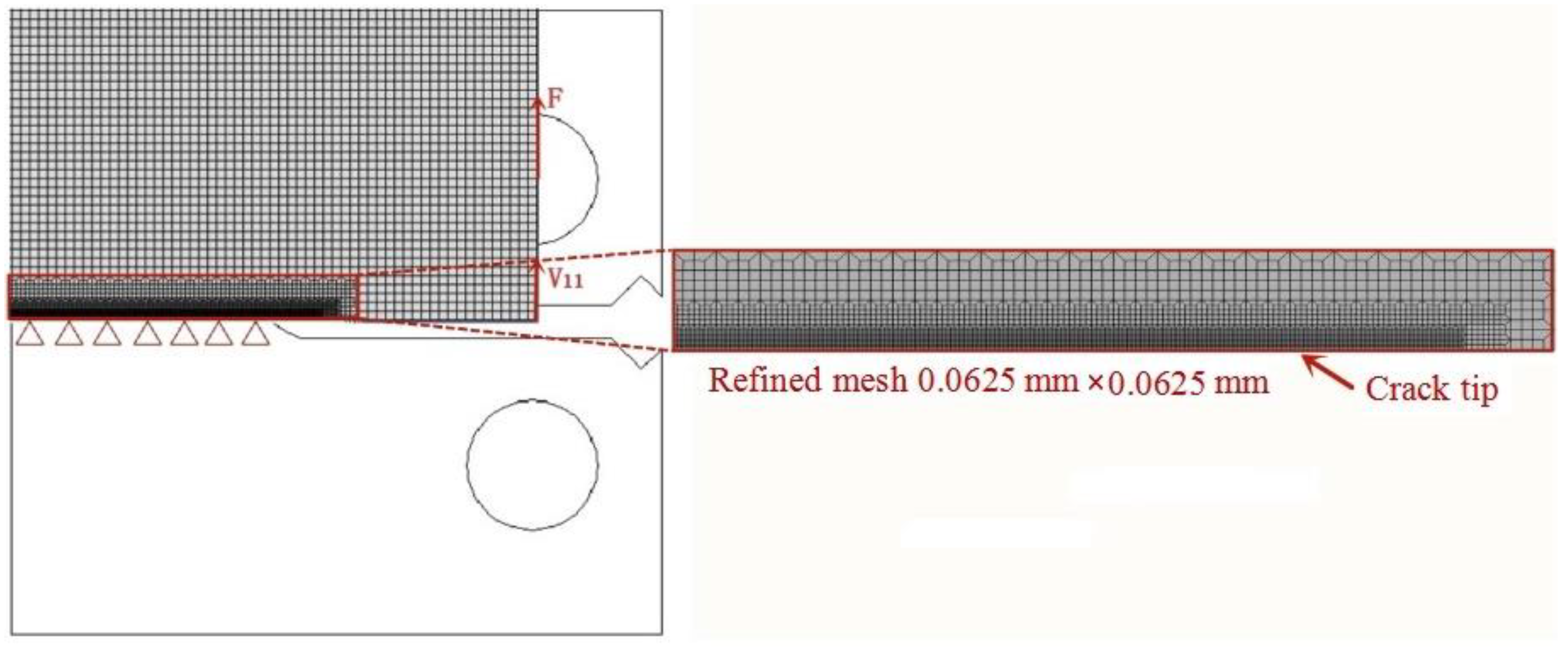
4.2. The Finite Element Model

The two-dimensional (2D) numerical model of the compact tension (CT) specimen is developed in ABAQUS. Due to symmetry, only the upper half was modeled with 5788 quadratic quadrilateral plane strain elements (CPE8R), as illustrated in Figure 5. The mesh size surrounding the fracture tip and region of crack extension is refined in the expected crack propagation domain, where the characteristic element size is 0.0625 mm. The length scale parameter $l$ is normally taken two times the characteristic element length around the fracture route [30]. We adopt a length scale 10 times larger than the characteristic element length to ensure enough elements within the process zone, $l=0.625 \mathrm{mm}$. The experimental tests are performed to verify the material parameters applied in the numerical model: Young’s modulus 202 GPa and Poisson’s ratio 0.3. The hydrogen damage coefficient x = 0.89 defined by Jiang and Carter [12] is applied. The diffusion coefficient $D$ = 4 × 10⁻⁵ mm²·s⁻¹ is examined, as reported by Wu et al. [44]. A velocity load F was applied at the loading hole and a data collection point was placed on the model loading line V_ll. We assumed the initial hydrogen concentration as $C\left(t=0\right)=C_0$ evenly distributed throughout the specimen. All exterior borders, including the crack surface, are prescribed a constant concentration, as specified by $C\left(t=0\right)=C_0$. The displacement rate was set to 10⁻⁹ mm·s⁻¹ for $t$ = 1 × 10⁷ s. This time step was selected for hydrogen redistribution inside the fracture process zone. With a magnitude $G_c\left(0\right)=78$ MPa·mm, the critical energy release rate without hydrogen offered the best fit to the data.

4.3. Result and Discussion

By using the presented model, the influential analyses of the hydrogen-assisted brittle fracture through varying phase-field parameters were conducted, and the results were compared with the experimental curves. As a result, for hydrogen-charged times of 12 h, 24 h, and 36 h, the initial hydrogen content values are 2.0 ppm, 7.0 ppm, and 11 ppm, respectively. Based on simulation and experimental data, the load-line displacements (V_ll) are depicted in Figure 6. Maximum response force and major curve characteristics are nearly identical in this figure and corroborate with experimental results, i.e., specimen load capacity declines with increasing hydrogen concentration. The HEDE mechanism adopted in this study to diffuse hydrogen into the phase-field model can be used numerically to calculate brittle fracture.

Figure 7, Figure 8 and Figure 9 illustrates the distributions of hydrostatic stress and hydrogen concentration along the fracture path at various load steps to determine hydrogen concentration at 7.0 ppm. The two distributions are found consistent, exhibiting a peak value near the crack tip, and the peak gradually increases with loading before crack initiation. With the displacement loading from 0.10 to 0.214 mm, the hydrogen concentration at the crack tip increases from 9.189 to 10.76 ppm and the corresponding hydrostatic stress are found as 2568 to 6034 MPa, respectively. The modeling results indicate that hydrostatic stress is the main cause of hydrogen diffusion at the crack tip. Hydrogen atoms concentrate in places with a high local hydrostatic stress gradient, as projected by the hydrogen diffusion flux formula Equation (19).

Fracture phase-field values and hydrogen concentrations near the crack tip before crack initiation are shown in Figure 10. As expected, hydrogen concentration is high on the positive hydrostatic stress, i.e., in the vicinity of the crack tip, while the crack begins to propagate when the phase-field values approach one. The maximum load and displacement are noted as 4810 N and 0.29 mm, respectively, which are less than the 6915 N and 0.39 mm values obtained in the absence of hydrogen. Fracture phase-field values and hydrogen concentrations near the crack tip after a certain degree of crack propagation are shown in Figure 11. Figure 11a shows the new crack surfaces as compared to the results shown in Figure (red contour level). The high hydrostatic stress zone moves with the crack tip, resulting in hydrogen concentration, and the peak moves to the newly formed crack surfaces during the crack propagation process. Figure 11b shows that hydrogen is transported ahead of the crack tip. When comparing crack tip hydrogen concentrations in Figure 10b and Figure 11b, the hydrogen concentration declines with fracture propagation. The hydrogen content drops from 14.30 ppm to 11.88 ppm during the crack propagation. The decrease in hydrogen concentration in the crack tip region is mainly related to the change of hydrostatic stress gradient in the region from crack initiation to crack propagation. In the process, the peak position of hydrostatic stress at the front of the crack tip moves with the crack propagation, and the strain gradient at the front area of the crack tip will be slightly lower than that at crack initiation. Therefore, the corresponding hydrostatic stress peak will also decrease slightly, thus resulting in a slight decrease in the hydrogen concentration at the front edge of the crack tip.

The distribution of the phase-field value after some amount of fracture propagation is shown in Figure 12, and the associated displacements are 0.38, 0.48, and 0.80 mm, respectively. At this point, the phase-field value reaches one, signaling the start of the crack. The red color indicates newly formed crack surfaces. The crack begins at the tip of the notch and rapidly propagates along the straight route. Meanwhile, the specimen undergoes a rapid load reduction.

5. Conclusions

This paper presents a hydrogen-assisted fracture methodology, which incorporates the HEDE mechanism into both hydrogen transport and a phase-field-based formulation to study hydrogen embrittlement. The numerical model is demonstrated through hydrogen-charged (CT) 45CrNiMoVA high-strength steel specimens and corroborates with the experimental results. The following are the main conclusions of this research:

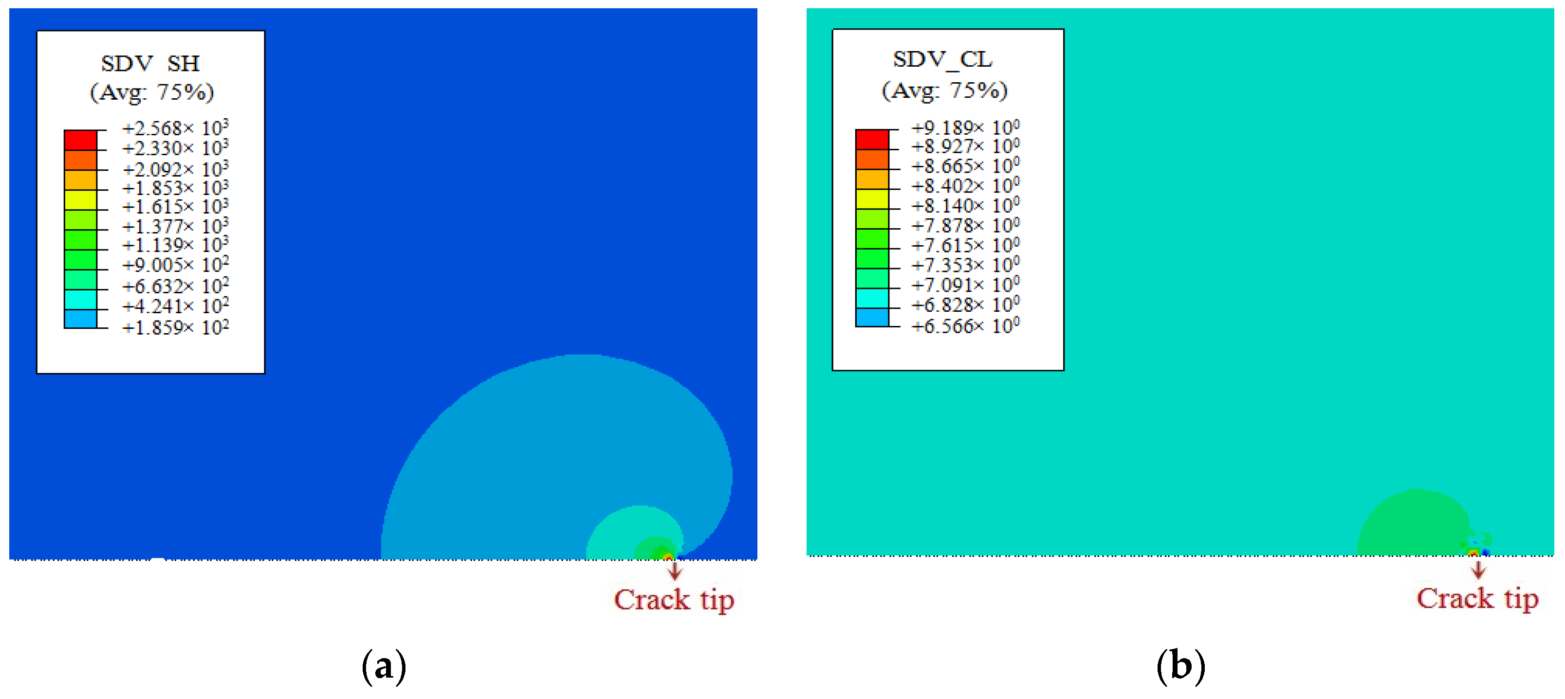
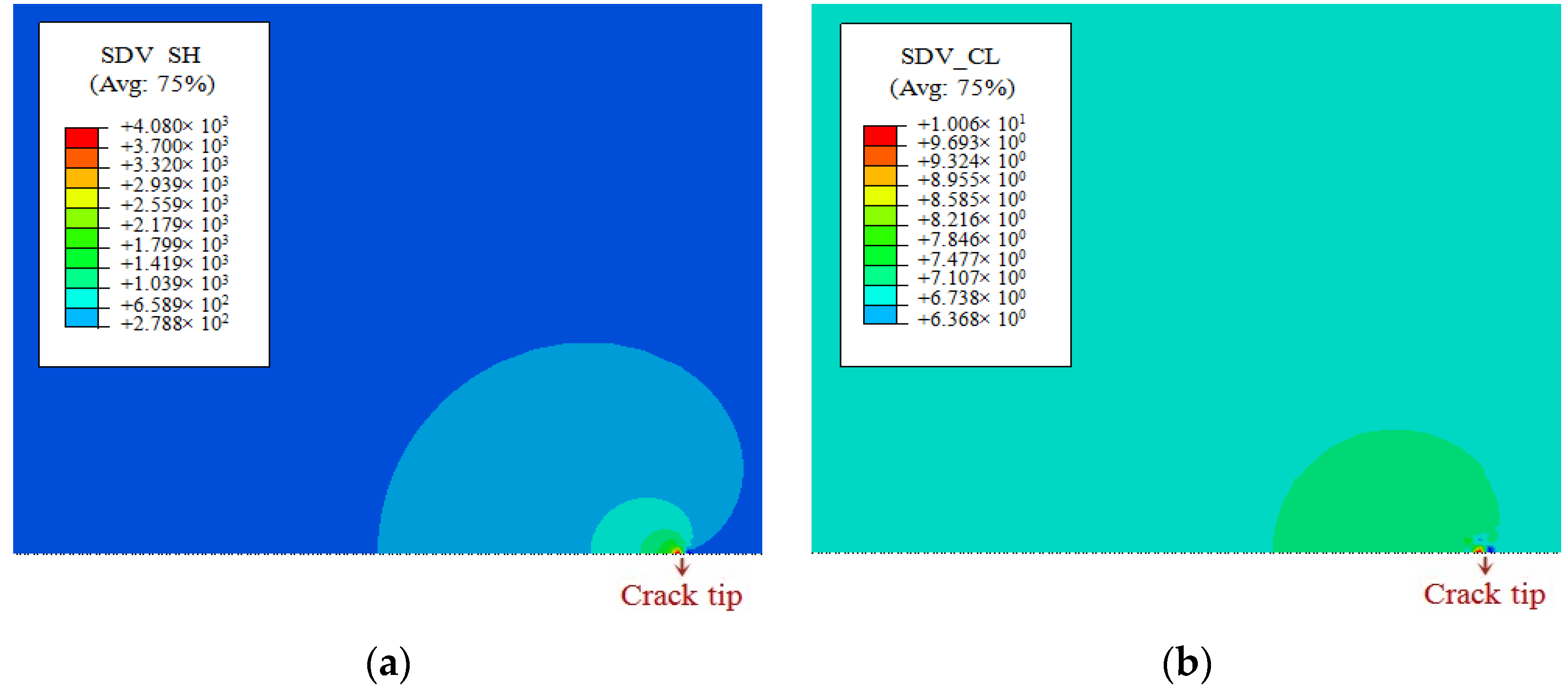
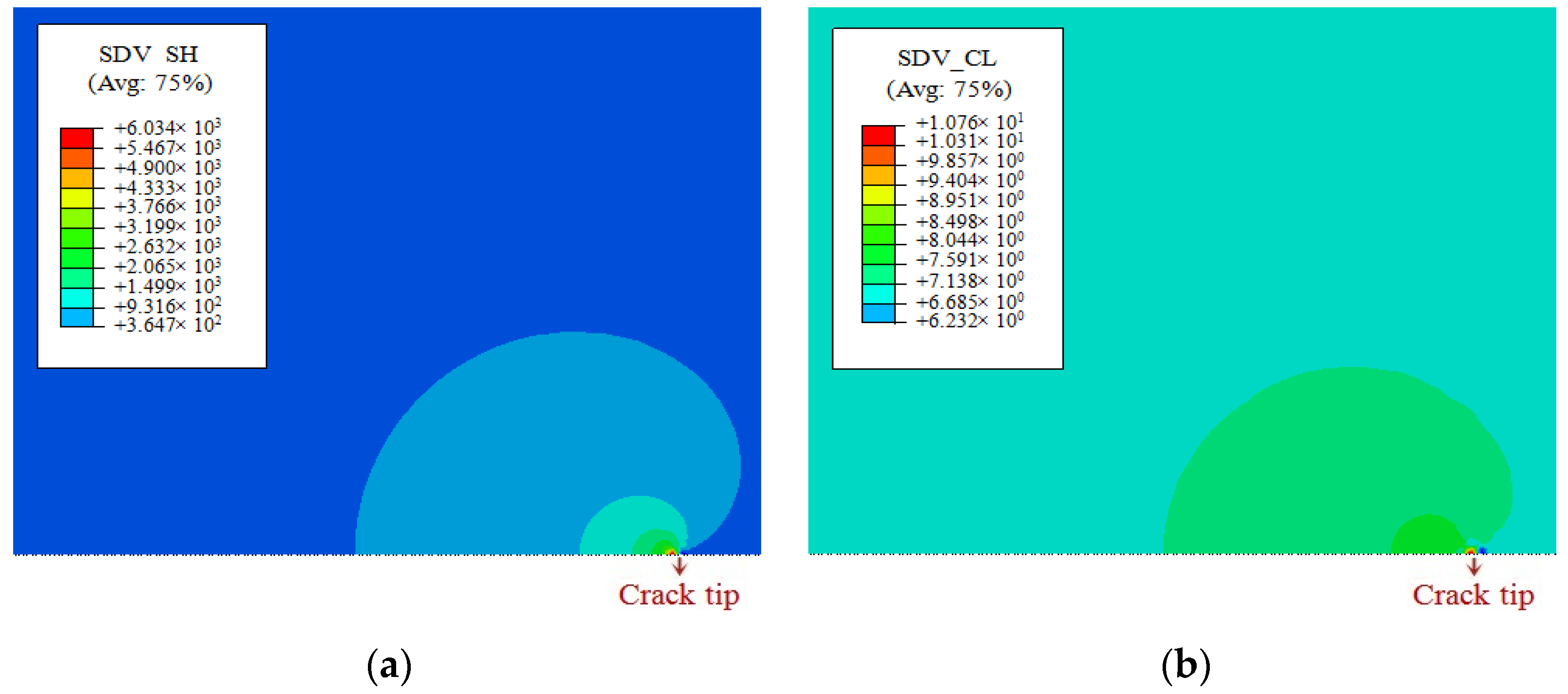
• The simulation results show that hydrogen accumulates near the crack tip due to positive hydrostatic stress and the peak increases gradually with loading before crack initiation.
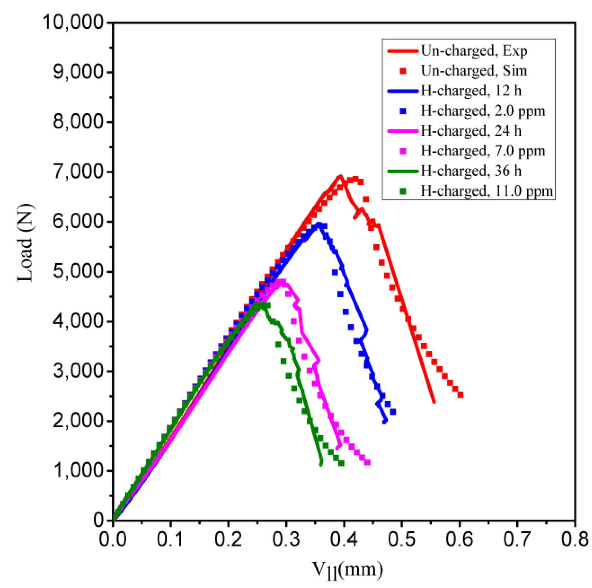
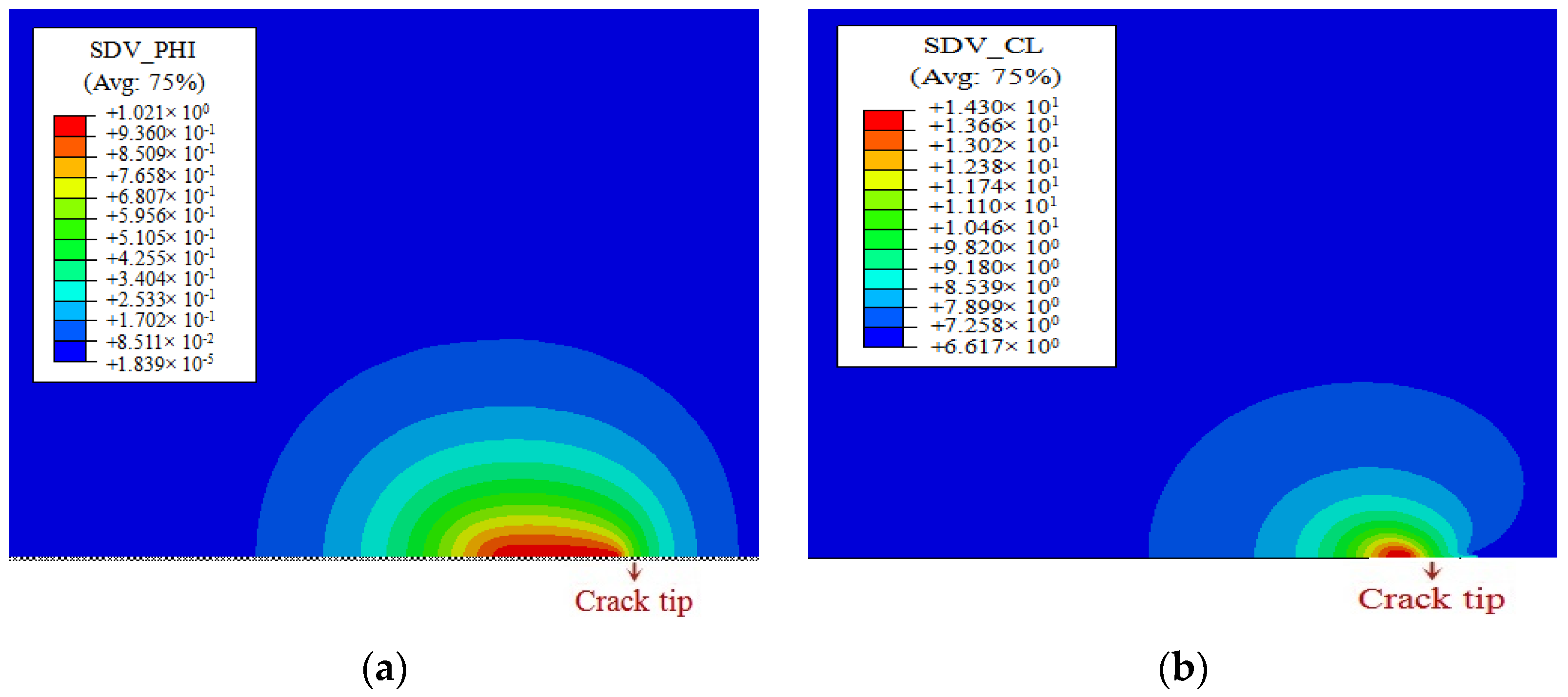
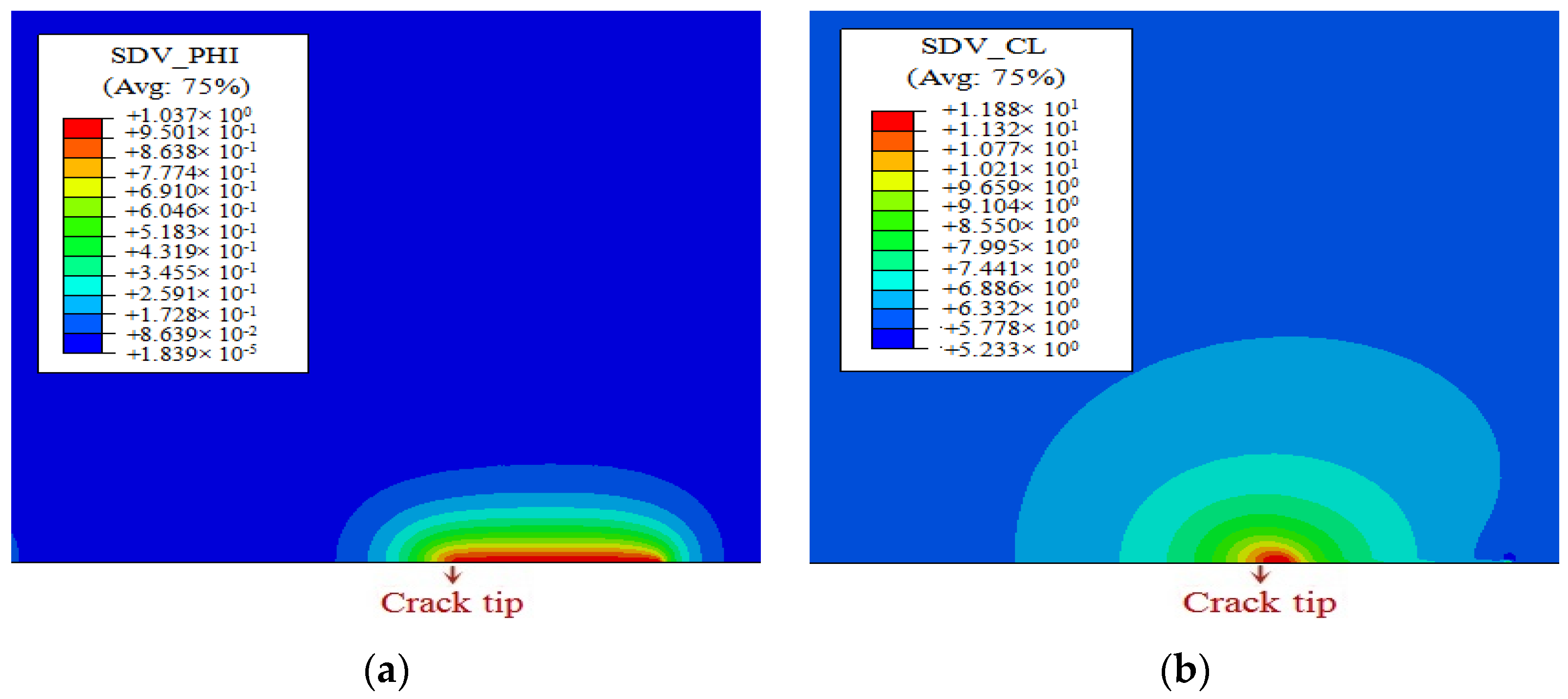
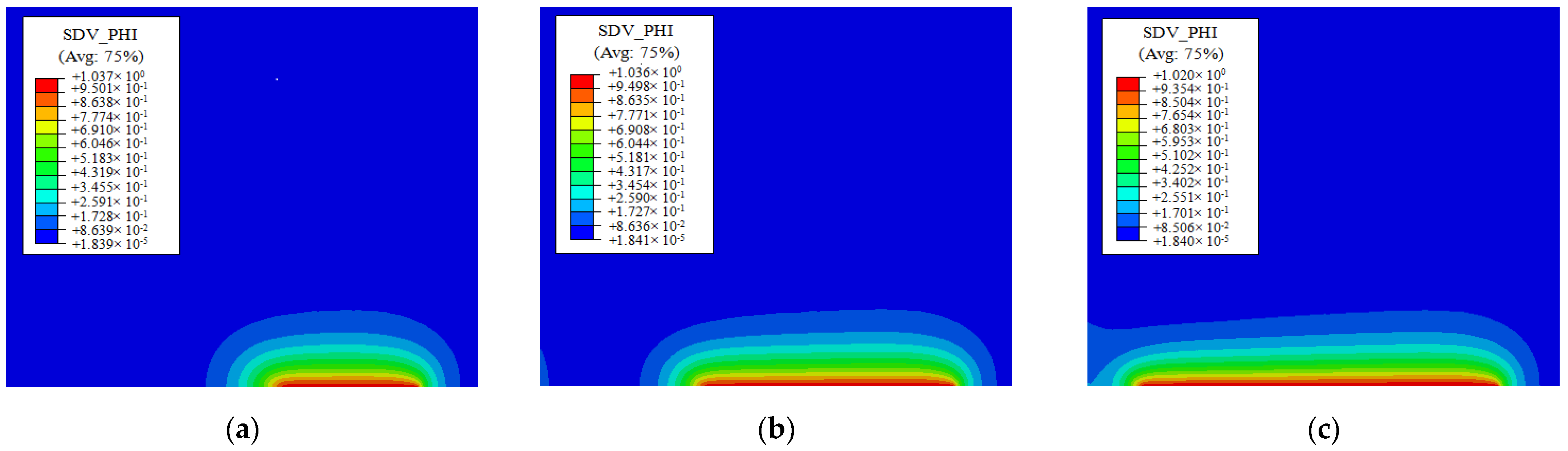
• The HEDE was implemented by determining the critical energy release rate drops when hydrogen concentration increases. In the presented simulations, the hydrogen concentration reaches a peak near the newly formed crack surfaces and gradually falls as the crack propagates. For load-line displacement curves, the maximum load-carrying ability decreases as the hydrogen content increases.
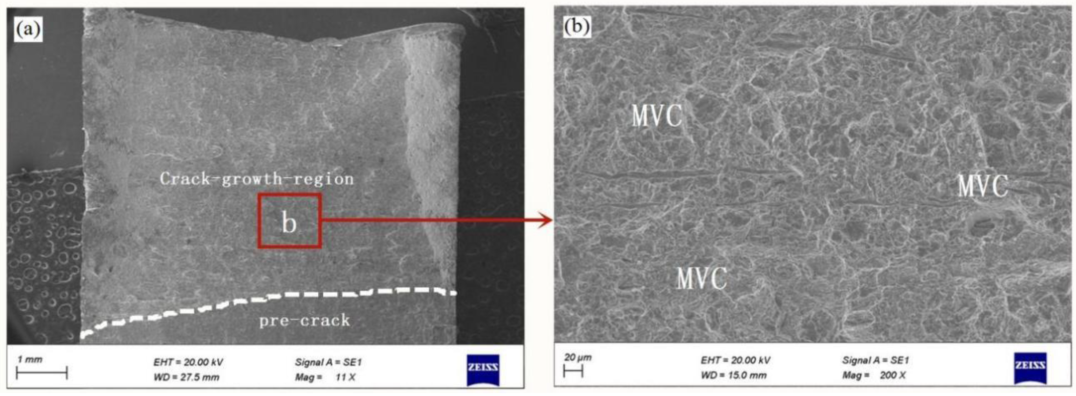
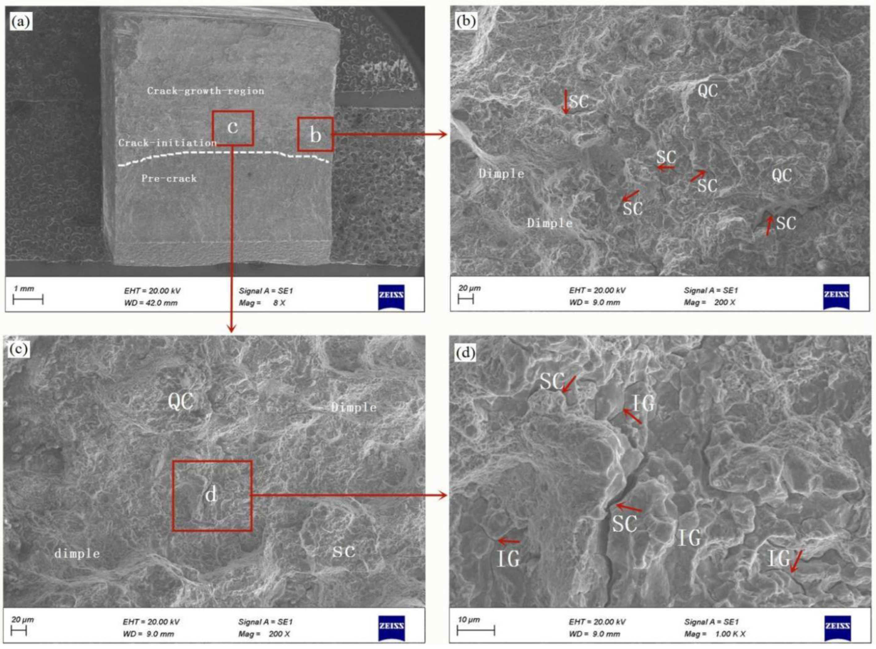
• The microstructural fracture mechanism of the hydrogen-charged 45CrNiMoVA high-strength steel compact-tension (CT) specimens demonstrate a brittle mixed fracture mode of QC and IG fracture that is consistent with the HEDE mechanism in the suggested model.
• The simulated load-line displacement curves show good agreement with computational and experimental curves. The model quantitatively estimates the initial hydrogen level. The proposed model provides a numerical tool for predicting the mechanical reaction of materials that are subjected to hydrogen-assisted brittle fracture, provided that the mechanical properties and phase-field model parameters are properly calibrated in advance.

The hydrogen-enhanced localized plasticity (HELP) is not accounted for in this model. To accurately forecast the hydrogen-assisted fracture ductile to brittle transition, this will be considered in future research.

References

1. Johnson, W.H. On some remarkable changes produced in iron and steel by the action of hydrogen and acids. Nature 1875, 11, 393. [Google Scholar] [CrossRef]
2. Wang, M.; Akiyama, E.; Tsuzaki, K. Determination of the critical hydrogen concentration for delayed fracture of high strength steel by constant load test and numerical calculation. Corros. Sci. 2006, 48, 2189–2202. [Google Scholar] [CrossRef]
3. Yatabe, H.; Yamada, K.; de Los, E.R.; Miller, K.J. Formation of hydrogen-assisted intergranular cracks in high strength steels. Fatigue Fract. Eng. Mater. Struct. 1995, 18, 377–384. [Google Scholar] [CrossRef]
4. Birnbaum, H.K.; Sofronis, P. Hydrogen-enhanced localized plasticity-a mechanism for hydrogen-related fracture. Mater. Sci. Eng. A 1994, 176, 191–202. [Google Scholar] [CrossRef]
5. Sofronis, P.; Liang, Y.; Aravas, N. Hydrogen induced shear localization of the plastic flow in metals and alloys. Eur. J. Mech. A/Solids 2001, 20, 857–872. [Google Scholar] [CrossRef]
6. Liang, Y.; Sofronis, P.; Aravas, N. On the effect of hydrogen on plastic instabilities in metals. Acta Mater. 2003, 51, 2717–2730. [Google Scholar] [CrossRef]
7. Ahn, D.C.; Sofronis, P.; Dodds, R.H. On hydrogen-induced plastic flow localization during void growth and coalescence. Int. J. Hydrogen Energy 2007, 32, 3734–3742. [Google Scholar] [CrossRef]
8. Pfeil, L.B. The effect of occluded hydrogen on the tensile strength of iron. Proc. R. Soc. Lond. Ser. A Contain. Pap. Math. Phys. Charact. 1926, 112, 182–195. [Google Scholar]
9. Troiano, A.R. The role of hydrogen and other interstitials in the mechanical behaviour of metals. Trans. ASM 1960, 52, 54–80. [Google Scholar]
10. Gerberich, W.W.; Oriani, R.A.; Lji, M.J.; Chen, X.; Foecke, T. The necessity of both plasticity and brittleness in the fracture thresholds of iron. Philos. Mag. A Phys. 1991, 63, 363–376. [Google Scholar] [CrossRef]
11. Oriani, R.A. A mechanistic theory of hydrogen embrittlement of steels. Ber Bunsen Phys. Chem. 1972, 76, 848–857. [Google Scholar]
12. Jiang, D.E.; Carter, E.A. First principles assessment of ideal fracture energies of materials with mobile impurities: Implications for hydrogen embrittlement of metals. Acta Mater. 2004, 52, 4801–4807. [Google Scholar] [CrossRef]
13. Serebrinsky, A.; Carter, E.A.; Ortiz, M. A quantum-mechanically informed continuum model of hydrogen embrittlement. J. Mech. Phys. Solids 2004, 52, 2403–2430. [Google Scholar] [CrossRef]
14. Jemblie, L.; Olden, V.; Mainçon, P.; Akselsen, O.M. Cohesive zone modelling of hydrogen induced cracking on the interface of clad steel pipes. Int. J. Hydrogen Energy 2017, 42, 28622–28634. [Google Scholar] [CrossRef]
15. Sobhaniaragh, B.; Afzalimir, S.H.; Ruggieri, C. Towards the prediction of hydrogen–induced crack growth in high-graded strength steels. Thin-Walled Struct. 2021, 159, 107245. [Google Scholar] [CrossRef]
16. Li, Y.; Zhang, K.; Lu, D.; Zeng, B. Hydrogen-assisted brittle fracture behavior of low alloy 30CrMo steel based on the combination of experimental and numerical analyses. Materials 2021, 14, 3711. [Google Scholar] [CrossRef] [PubMed]
17. Griffith, A.A. The phenomena of rupture and flow in solids. Philos. Trans. R Soc. Lond. A Math. Phys. Sci. 1921, 221, 163–198. [Google Scholar]
18. Francfort, G.A.; Marigo, J.J. Revisiting brittle fracture as an energy minimization problem. J. Mech. Phys. Solids 1998, 46, 1319–1342. [Google Scholar] [CrossRef]
19. Bourdin, B.; Francfort, G.A.; Marigo, J.J. Numerical experiments in revisited brittle fracture. J. Mech. Phys. Solids 2000, 48, 797–826. [Google Scholar] [CrossRef]
20. Bourdin, B.; Francfort, G.A.; Marigo, J.J. The Variational Approach to Fracture. J. Elast. 2008, 91, 5–148. [Google Scholar] [CrossRef]
21. Miehe, C.; Hofacker, M.; Welschinger, F. A phase field model for rate independent crack propagation: Robust algorithmic implementation based on operator splits. Comput. Methods Appl. Mech. Eng. 2010, 199, 2765–2778. [Google Scholar] [CrossRef]
22. Miehe, C.; Schänzel, L.M.; Ulmer, H. Phase field modeling of fracture in multiphysics problems. Part I. Balance of crack surface and failure criteria for brittle crack propagation in thermo-elastic solids. Comput. Methods Appl. Mech. Eng. 2015, 294, 449–485. [Google Scholar] [CrossRef]
23. Miehe, C.; Hofacker, M.; Schänzel, L.M.; Aldakheel, F. Phase field modeling of fracture in multi-physics problems. Part II. Coupled brittle-to-ductile failure criteria and crack propagation in thermo-elastic-plastic solids. Comput. Methods Appl. Mech. Eng. 2015, 294, 486–522. [Google Scholar] [CrossRef]
24. Ambati, M.; Gerasimov, T.; De Lorenzis, L. Phase-field modeling of ductile fracture. Comput. Mech. 2015, 55, 1017–1040. [Google Scholar] [CrossRef]
25. Ambati, M.; Kruse, R.; De Lorenzis, L. A phase-field model for ductile fracture at finite strains and its experimental verification. Comput. Mech. 2016, 57, 149–167. [Google Scholar] [CrossRef]
26. Philip, K.K.; Christian, F.N.; Martínez-Pañeda, E. A phase field model for elastic-gradient-plastic solids undergoing hydrogen embrittlement. J. Mech. Phys. Solids 2020, 143, 104093. [Google Scholar]
27. Martínez-Pañeda, E.; Golahmar, A.; Christian, F.N. A phase field formulation for hydrogen assisted cracking. Comput. Methods Appl. Mech. Eng. 2018, 342, 742–761. [Google Scholar] [CrossRef] [Green Version]
28. Wu, J.Y.; Mandal, T.K.; Nguyen, V.P. A phase-field regularized cohesive zone model for hydrogen assisted cracking. Comput. Methods Appl. Mech. Eng. 2020, 358, 112614. [Google Scholar] [CrossRef]
29. Martínez-Pañeda, E.; Harris, Z.D.; Fuentes-Alonso, S.; Scully, J.R.; Burns, J.T. On the suitability of slow strain rate tensile testing for assessing hydrogen embrittlement susceptibility. Corros. Sci. 2020, 163, 108291. [Google Scholar] [CrossRef] [Green Version]
30. Molnár, G.; Gravouil, A. 2D and 3D Abaqus implementation of a robust staggered phase-field solution for modeling brittle fracture. Finite Elements Anal. Des. 2017, 130, 27–38. [Google Scholar] [CrossRef] [Green Version]
31. Miehe, C.; Welschinger, F.; Hofacker, M. Thermodynamically consistent phase-field models of fracture: Variational principles and multi-fifield fe implementations. Int. J. Numer. Methods Eng. 2010, 10, 1273–1311. [Google Scholar] [CrossRef]
32. Crank, J. The Mathematics of Diffusion; Oxford University Press: London, UK, 1979. [Google Scholar]
33. Hirth, J.P. Effects of hydrogen on the properties of iron and steel. Metall. Mater. Trans. A 1980, 6, 861–890. [Google Scholar] [CrossRef]
34. Alvaro, A.; Jensen, I.T.; Kheradmand, N.; Løvvik, O.M.; Olden, V. Hydrogen embrittlement in nickel, visited by first principles modeling, cohesive zone simulation and nanomechanical testing. Int. J. Hydrogen Energy 2015, 47, 16892–16900. [Google Scholar] [CrossRef]
35. Hondros, E.; Seah, M. The theory of grain boundary segregation in terms of surface adsorption analogues. Metall. Mater. Trans. A 1977, 8, 1363–1371. [Google Scholar] [CrossRef]
36. Kotake, H.; Matsumoto, R.; Taketomi, S.; Miyazaki, N. Transient hydrogen diffusion analyses coupled with crack-tip plasticity under cyclic loading. Int. J. Press. Vessel. Pip. 2008, 85, 540–549. [Google Scholar] [CrossRef]
37. ASTM. E1820-09; Standard Test Method for Measurement of Fracture Toughness. ASTM: Philadelphia, PA, USA, 2016.
38. Li, X.F.; Zhang, J.; Chen, J.; Shen, S.; Yang, G.X.; Wang, T.J.; Song, X.L. Effect of aging treatment on hydrogen embrittlement of PH 13-8 Mo martensite stainless steel. Mater. Sci. Eng. A Struct. Mater. 2016, 651, 474–485. [Google Scholar] [CrossRef]
39. Wu, S.J.; Sung, S.J.; Pan, J.; Lam, P.S.; Morgan, M.; Korinko, P. Modeling of Crack Extensions in Arc-Shaped Specimens of Hydrogen-Charged Austenitic Stainless Steels Using Cohesive Zone Model. Press. Vessel. Pip. Conf. 2018, 7, 15–20. [Google Scholar]
40. ISO12135; International Standard of Unified Method of Test for the Determination of Quasistatic Fracture Toughness. ISO 2002; ISO Technical Committees: Geneva, Switzerland, 2002; pp. 65–67.
41. Yao, Y.; Cai, L.X.; Bao, C.; Jiang, H. The fined COD transform formula for CT specimens to investigate material fracture toughness. AMM 2012, 188, 11–16. [Google Scholar] [CrossRef]
42. Nagao, A.; Smith, C.D.; Dadfarnia, M.; Sofronis, P.; Robertson, L.M. The role of hydrogen in hydrogen embrittlement fracture of lath martensitic steel. Acta Mater. 2012, 60, 5182–5189. [Google Scholar] [CrossRef]
43. Nagao, A.; Martin, M.L.; Dadfarnia, M.; Sofronis, P.; Robertson, I.M. The effect ofnanosized (Ti, Mo)C precipitates on hydrogen embrittlement of tempered lath martensitic steel. Acta Mater. 2014, 74, 244–254. [Google Scholar] [CrossRef]
44. Wu, W.J.; Wang, Y.F.; Tao, P.; Li, F.X.; Gong, J.M. Cohesive zone modeling of hydrogen-induced delayed intergranular fracture in high strength steels. Results Phys. 2018, 11, 591–598. [Google Scholar] [CrossRef]
Figure 1. (a) The hydrogen coverage θ as a function of hydrogen concentration for a range of Gibbs free energy values of 10 kJ/mol to 60 kJ/mol; (b) hydrogen embrittlement parameter G C ( θ ) / G C ( 0 ) as a function of hydrogen concentration for a range of hydrogen damage factor χ values of 0.30 to 1.00 ( Δ G g 0 = 30   kJ / mol ).
Metals 12 01032 g001
Figure 2. (a) Geometry of CT specimen (unit: mm); (b) load-line displacement curves for CT specimen.
Metals 12 01032 g002
Figure 3. (a) Scanning electron microscopy (SEM) images for 45CrNiMoVA low alloy steel CT specimen, and (b) SEM high magnification image of the selected region in (a).
Metals 12 01032 g003
Figure 4. SEM images of the fracture surface of 45CrNiMoVA low alloy steel CT specimen H-charged for 36 h: (a) overview of the fracture surface; (b,c) high magnification SEM images of the indicated region in image (a); (d) high magnification SEM image of the indicated region in image (c); (red arrowheads indicate secondary cracks (SCs) and white arrowheads indicate tear ridges). QC: quasi-cleavage; IG: intergranular fracture; MVC: microvoid coalescence.
Metals 12 01032 g004
Figure 5. Finite element model for the (CT) specimen.
Metals 12 01032 g005
Figure 6. Load-line displacement curves for uncharged and hydrogen-charged CT specimens.
Metals 12 01032 g006
Figure 7. (a) Hydrostatic stress and (b) hydrogen concentration contours near the crack tip at u = 0.10 mm for C 0 = 7.0 ppm.
Metals 12 01032 g007
Figure 8. (a) Hydrostatic stress and (b) hydrogen concentration contours near the crack tip at u = 0.16 mm for C 0 = 7.0 ppm.
Metals 12 01032 g008
Figure 9. (a) Hydrostatic stress and (b) hydrogen concentration contours near the crack tip at u = 0.214 mm for C 0 = 7.0 ppm.
Metals 12 01032 g009
Figure 10. (a) Distributions of crack phase-field value and (b) hydrogen concentration at crack tip before the onset of crack initiation for C 0 = 7.0 ppm.
Metals 12 01032 g010
Figure 11. (a) Distributions of crack phase-field value and (b) hydrogen concentration at crack tip after some amount of crack propagation for C 0 = 7.0 ppm.
Metals 12 01032 g011
Figure 12. Distributions of crack phase-field value at crack tip after some amount of fracture propagation for C0 = 7.0 ppm: (a) u = 0.38 mm, (b) u = 0.48 mm, (c) u = 0.80 mm.
Metals 12 01032 g012