
A Particle Size Distribution Model for Tailings in Mine Backfill


Abstract
:1. Introduction
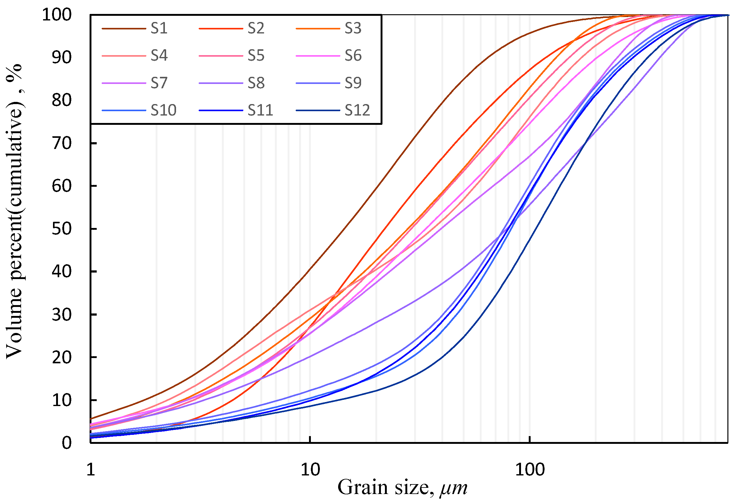
2. Materials
3. Mathematical Model
3.1. Definition of Coefficients
- Step 1: Three methods to determine Coefficient K
- (a).
- Method 1: The meaning of K value is the cumulative fraction of particles when the particle size reaches infinity. Therefore, the approximate value is Approach to 100%. It is means K = 100 (Excluding percent sign, the same below).
- (b).
- Method 2: According to Equation (2), three equidistant points are selected to eliminate the coefficients A and B. The value K can be calculated by solving the Equation (4). The equidistant points can be 37 μm, 74 μm, and 150 μm.where N0, N1, and N2 are the cumulative percentage values of particles passing 37 μm, 74 μm, and 150 μm. It should be pointed out that the K value can be calculated for N0, N1 and N2 of any equidistant points. The above value method can cover most of the particle size range of tailings for common tailings, and the value is relatively reasonable.
- (c).
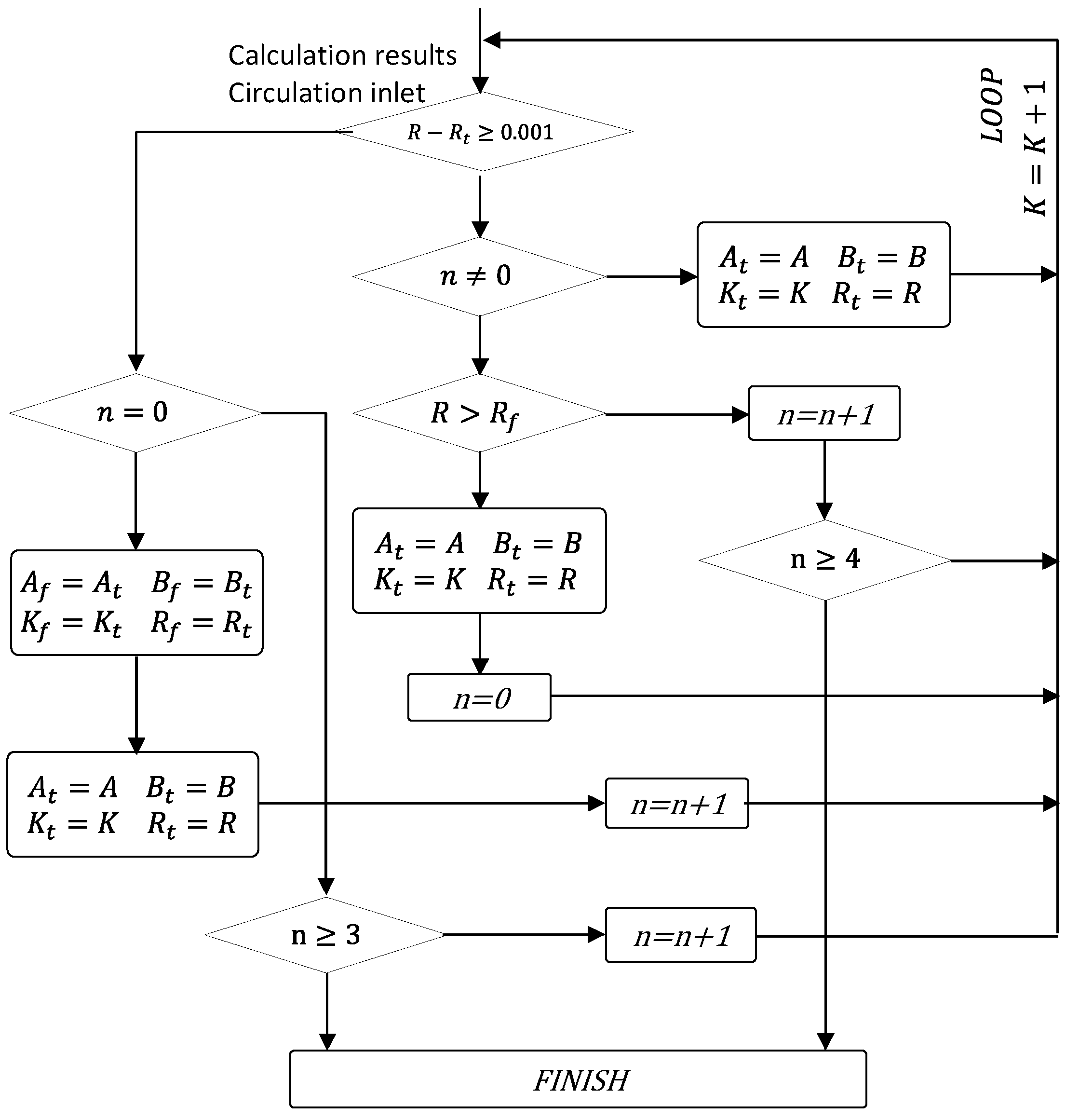
- Method 3: The K value is optimal fitting solved by loop iterative calculation, which will be discussed in Section 3.2.
- Step 2: Take points and linear regression to obtain coefficients A and B
- Step 3: Error analysis
3.2. Iterative Analysis for the Optimal Fitting Coefficient
3.3. Coefficients Interpretation
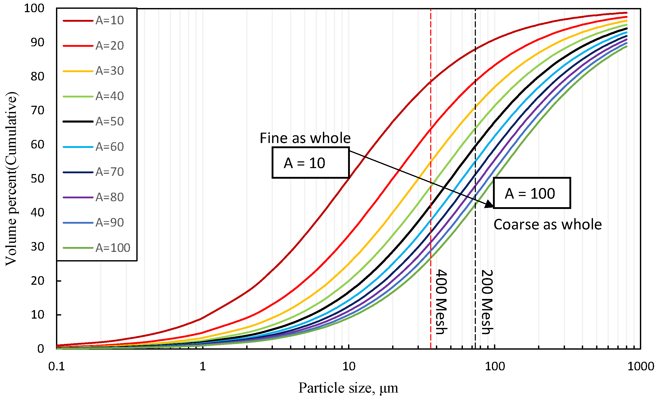
- (a)
- Coefficient A reflects the average particle size
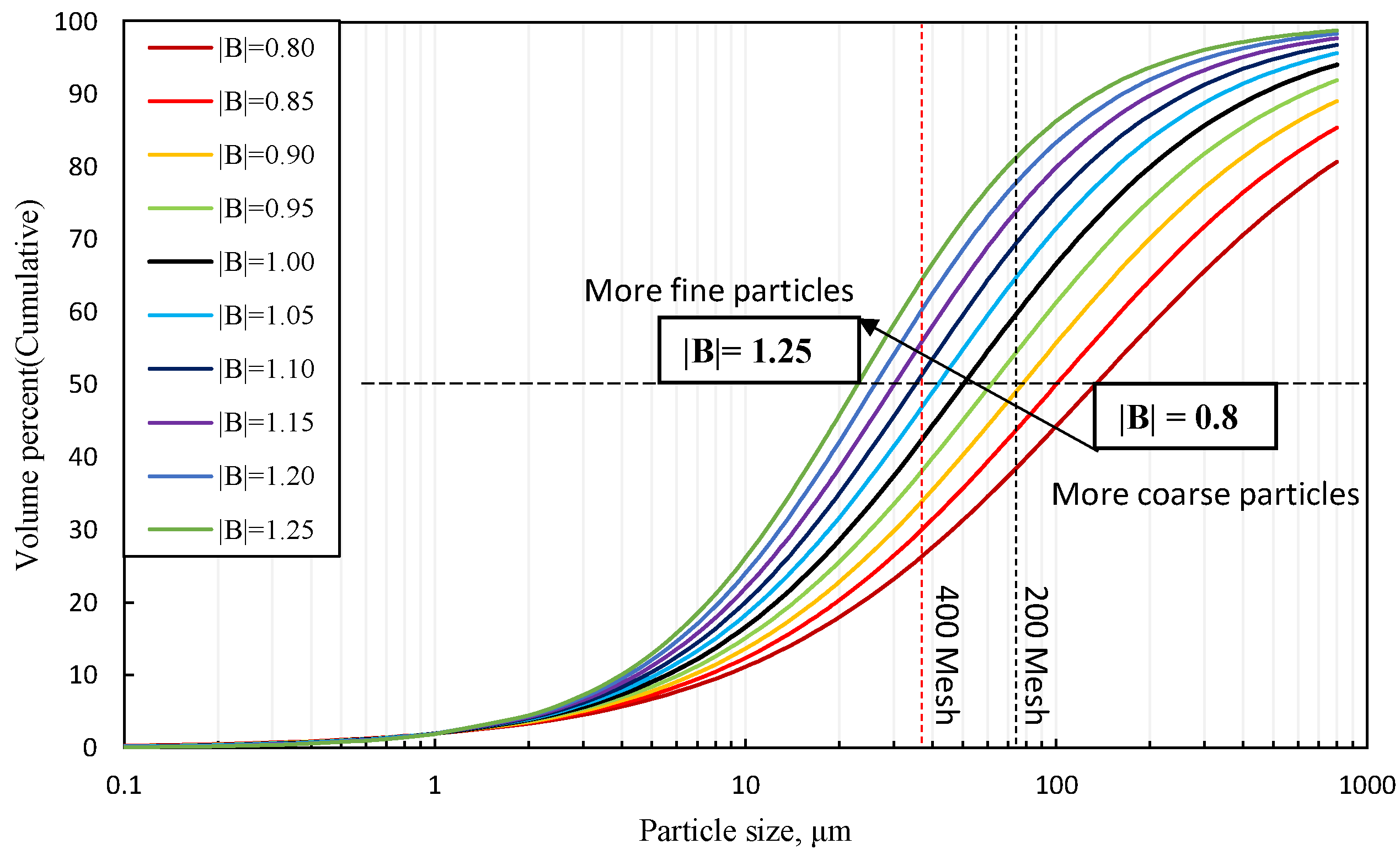
- (b)
- Coefficient B represents the proportion of coarse and fine tailings
- (c)
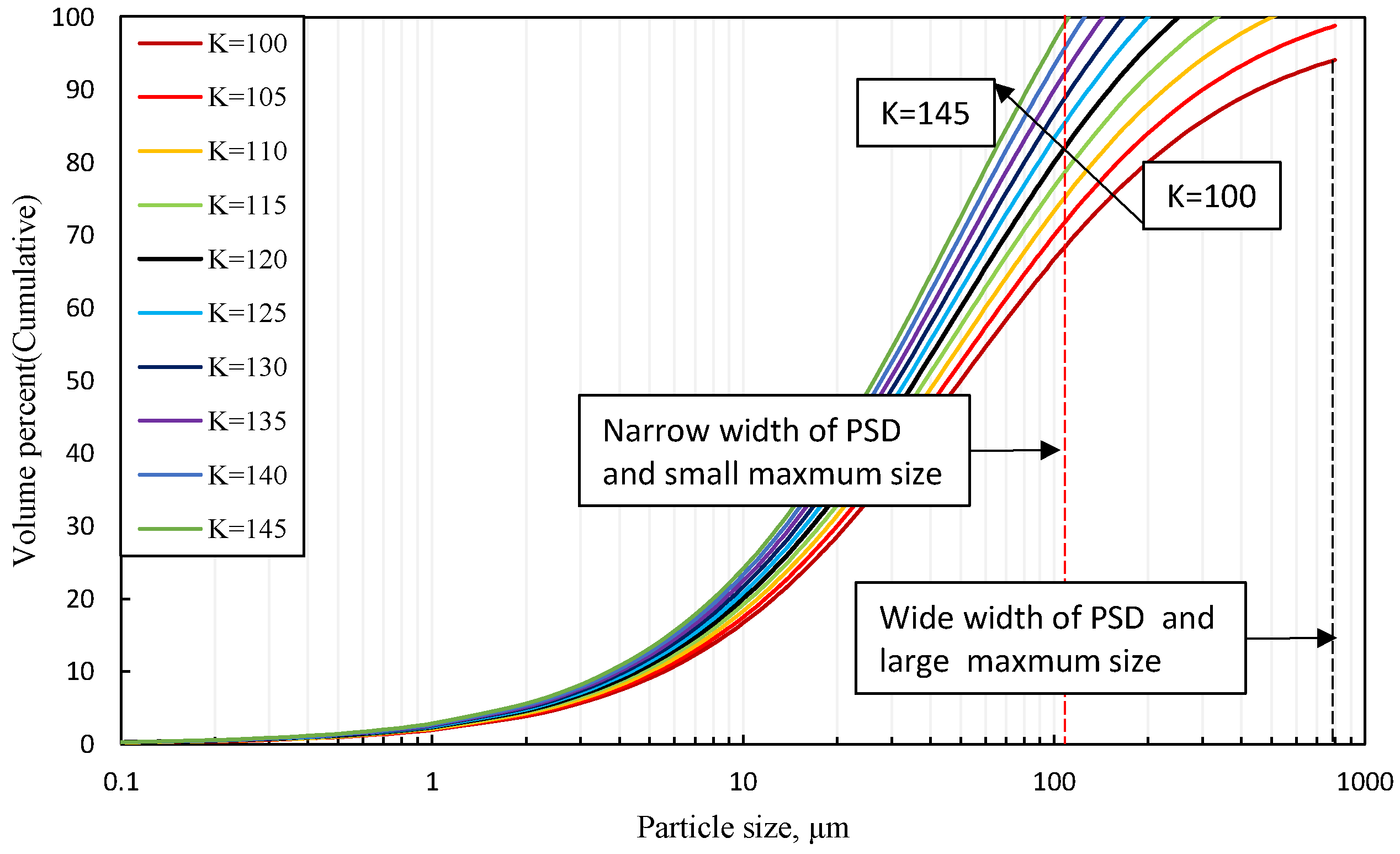
- Coefficient K represents the width of particle distribution
4. Validation and Discussion
5. Conclusions
Author Contributions
Funding
Data Availability Statement
Conflicts of Interest
References
- Jones, H.; Boger, D.V. Sustainability and Waste Management in the Resource Industries. Ind. Eng. Chem. Res. 2012, 51, 10057–10065. [Google Scholar] [CrossRef]
- Franks, D.M.; Boger, D.V.; Côte, C.M.; Mulligan, D.R. Sustainable development principles for the disposal of mining and mineral processing wastes. Resour. Policy 2011, 36, 114–122. [Google Scholar] [CrossRef]
- Sivakugan, N.; Veenstra, R.; Naguleswaran, N. Underground Mine Backfilling in Australia Using Paste Fills and Hydraulic Fills. Int. J. Geosynth. Ground Eng. 2015, 1, 18. [Google Scholar] [CrossRef] [Green Version]
- Birat, J.-P. Society, Materials, and the Environment: The Case of Steel. Metals 2020, 10, 331. [Google Scholar] [CrossRef] [Green Version]
- El-Batsh, H.M.; Doheim, M.A.; Hassan, A.F. On the application of mixture model for two-phase flow induced corrosion in a complex pipeline configuration. Appl. Math. Model. 2012, 36, 5686–5699. [Google Scholar] [CrossRef]
- Behera, S.K.; Mishra, D.; Singh, P.; Mishra, K.; Mandal, S.K.; Ghosh, C.; Kumar, R.; Mandal, P.K. Utilization of mill tailings, fly ash and slag as mine paste backfill material: Review and future perspective. Constr. Build. Mater. 2021, 309, 125120. [Google Scholar] [CrossRef]
- Ting, X.; Xinzhuo, Z.; Miedema, S.A.; Xiuhan, C. Study of the characteristics of the flow regimes and dynamics of coarse particles in pipeline transportation. Powder Technol. 2019, 347, 148–158. [Google Scholar] [CrossRef]
- Mourinha, C.; Palma, P.; Alexandre, C.; Cruz, N.; Rodrigues, S.M.; Alvarenga, P. Potentially Toxic Elements’ Contamination of Soils Affected by Mining Activities in the Portuguese Sector of the Iberian Pyrite Belt and Optional Remediation Actions: A Review. Environments 2022, 9, 11. [Google Scholar] [CrossRef]
- Liu, Q.; Liu, D.; Tian, Y.; Liu, X. Numerical simulation of stress-strain behaviour of cemented paste backfill in triaxial compression. Eng. Geol. 2017, 231, 165–175. [Google Scholar] [CrossRef]
- Zhao, Y.; Taheri, A.; Karakus, M.; Deng, A.; Guo, L. The Effect of Curing under Applied Stress on the Mechanical Performance of Cement Paste Backfill. Minerals 2021, 11, 1107. [Google Scholar] [CrossRef]
- Xu, W.; Cao, P.; Tian, M. Strength Development and Microstructure Evolution of Cemented Tailings Backfill Containing Different Binder Types and Contents. Minerals 2018, 8, 167. [Google Scholar] [CrossRef] [Green Version]
- Le, Z.-H.; Yu, Q.-L.; Pu, J.-Y.; Cao, Y.-S.; Liu, K. A Numerical Model for the Compressive Behavior of Granular Backfill Based on Experimental Data and Application in Surface Subsidence. Metals 2022, 12, 202. [Google Scholar] [CrossRef]
- Öhlander, B.; Chatwin, T.; Alakangas, L. Management of Sulfide-Bearing Waste, a Challenge for the Mining Industry. Minerals 2012, 2, 1–10. [Google Scholar] [CrossRef]
- Wu, D.; Yang, B.; Liu, Y. Pressure drop in loop pipe flow of fresh cemented coal gangue–fly ash slurry: Experiment and simulation. Adv. Powder Technol. 2015, 26, 920–927. [Google Scholar] [CrossRef]
- Li, M.-Z.; He, Y.-P.; Liu, Y.-D.; Huang, C. Pressure drop model of high-concentration graded particle transport in pipelines. Ocean Eng. 2018, 163, 630–640. [Google Scholar] [CrossRef]
- Wilson, K.C. Deposition limit nomograms for particles of various densities in pipeline flow. Hydrotransport 1979, 1, 1–12. [Google Scholar]
- Kesimal, A.; Yilmaz, E.; Ercikdi, B.; Alp, I.; Deveci, H. Effect of properties of tailings and binder on the short-and long-term strength and stability of cemented paste backfill. Mater. Lett. 2005, 59, 3703–3709. [Google Scholar] [CrossRef]
- Libos, I.L.S.; Cui, L. Effects of curing time, cement content, and saturation state on mode-I fracture toughness of cemented paste backfill. Eng. Fract. Mech. 2020, 235, 107174. [Google Scholar] [CrossRef]
- Zhao, Y.; Taheri, A.; Karakus, M.; Chen, Z.; Deng, A. Effects of water content, water type and temperature on the rheological behaviour of slag-cement and fly ash-cement paste backfill. Int. J. Min. Sci. Technol. 2020, 30, 271–278. [Google Scholar] [CrossRef]
- Peng, X.; Guo, L.; Liu, G.; Yang, X.; Chen, X. Experimental Study on Factors Influencing the Strength Distribution of In Situ Cemented Tailings Backfill. Metals 2021, 11, 2059. [Google Scholar] [CrossRef]
- Wilson, K.C.; Clift, R.; Addie, G.R.; Maffett, J. Effect of broad particle grading on slurry stratification ratio and scale-up-ScienceDirect. Powder Technol. 1990, 61, 165–172. [Google Scholar] [CrossRef]
- Guo, W.; Han, Y.; Gao, P.; Tang, Z. Effect of operating conditions on the particle size distribution and specific energy input of fine grinding in a stirred mill: Modeling cumulative undersize distribution. Miner. Eng. 2022, 176, 107347. [Google Scholar] [CrossRef]
- Quezada, G.R.; Ramos, J.; Jeldres, R.I.; Robles, P.; Toledo, P.G. Analysis of the flocculation process of fine tailings particles in saltwater through a population balance model. Sep. Purif. Technol. 2020, 237, 116319. [Google Scholar] [CrossRef]
- Guo, Z.; Qiu, J.; Jiang, H.; Zhang, S.; Ding, H. Improving the performance of superfine-tailings cemented paste backfill with a new blended binder. Powder Technol. 2021, 394, 149–160. [Google Scholar] [CrossRef]
- Zanko, L.M.; Niles, H.B.; Oreskovich, J.A. Mineralogical and microscopic evaluation of coarse taconite tailings from Minnesota taconite operations. Regul. Toxicol. Pharmacol. 2008, 52 (Suppl. 1), S51–S65. [Google Scholar] [CrossRef]
- Uzi, A.; Levy, A. Flow characteristics of coarse particles in horizontal hydraulic conveying. Powder Technol. 2018, 326, 302–321. [Google Scholar] [CrossRef]
- Zhang, B.; Xin, J.; Liu, L.; Guo, L.; Song, K.-I. An Experimental Study on the Microstructures of Cemented Paste Backfill during Its Developing Process. Adv. Civ. Eng. 2018, 2018, 1–10. [Google Scholar] [CrossRef]
- Singh, J.P.; Kumar, S.; Mohapatra, S.K. Modelling of two phase solid-liquid flow in horizontal pipe using computational fluid dynamics technique. Int. J. Hydrogen Energy 2017, 42, 20133–20137. [Google Scholar] [CrossRef]
- Qi, C.; Chen, Q.; Fourie, A.; Zhao, J.; Zhang, Q. Pressure drop in pipe flow of cemented paste backfill: Experimental and modeling study. Powder Technol. 2018, 333, 9–18. [Google Scholar] [CrossRef]
- Wu, D.; Yang, B.; Liu, Y. Transportability and pressure drop of fresh cemented coal gangue-fly ash backfill (CGFB) slurry in pipe loop. Powder Technol. 2015, 284, 218–224. [Google Scholar] [CrossRef]
- Li, M.; He, Y.; Liu, Y.; Huang, C. Effect of interaction of particles with different sizes on particle kinetics in multi-sized slurry transport by pipeline. Powder Technol. 2018, 338, 915–930. [Google Scholar] [CrossRef]
- Lu, G.; Fall, M.; Yang, Z. An evolutive bounding surface plasticity model for early-age cemented tailings backfill under cyclic loading. Soil Dyn. Earthq. Eng. 2019, 117, 339–356. [Google Scholar] [CrossRef]
- Liu, L.; Fang, Z.; Wu, Y.; Lai, X.; Wang, P.; Song, K.-I. Experimental investigation of solid-liquid two-phase flow in cemented rock-tailings backfill using Electrical Resistance Tomography. Constr. Build. Mater. 2018, 175, 267–276. [Google Scholar] [CrossRef]
- Matoušek, V.; Chára, Z.; Konfršt, J.; Novotný, J. Experimental investigation on effect of stratification of bimodal settling slurry on slurry flow friction in pipe. Exp. Therm. Fluid Sci. 2022, 132, 110561. [Google Scholar] [CrossRef]
- Zhang, J.; Cheng, L.; Yuan, H.; Mei, N.; Yan, Z. Identification of viscosity and solid fraction in slurry pipeline transportation based on the inverse heat transfer theory. Appl. Therm. Eng. 2019, 163, 114328. [Google Scholar] [CrossRef]
- Adiguzel, D.; Bascetin, A. The investigation of effect of particle size distribution on flow behavior of paste tailings. J. Environ. Manag. 2019, 243, 393–401. [Google Scholar] [CrossRef]
- US Department of Commerce. NIST Recommended Practice Guide: Particle Size Characterization; National Institute of Standards and Technology: Gaithersburg, MD, USA, 2001.
- Zhu, J.; Wu, S.; Cheng, H.; Geng, X.; Liu, J. Response of Floc Networks in Cemented Paste Backfill to a Pumping Agent. Metals 2021, 11, 1906. [Google Scholar] [CrossRef]
- Kaushal, D.R.; Sato, K.; Toyota, T.; Funatsu, K.; Tomita, Y. Effect of particle size distribution on pressure drop and concentration profile in pipeline flow of highly concentrated slurry. Int. J. Multiph. Flow 2005, 31, 809–823. [Google Scholar] [CrossRef]
- Kaushal, D.R.; Thinglas, T.; Tomita, Y.; Kuchii, S.; Tsukamoto, H. CFD modeling for pipeline flow of fine particles at high concentration. Int. J. Multiph. Flow 2012, 43, 85–100. [Google Scholar] [CrossRef]
- Lang, L.; Song, K.-I.; Lao, D.; Kwon, T.-H. Rheological Properties of Cemented Tailing Backfill and the Construction of a Prediction Model. Materials 2015, 8, 2076–2092. [Google Scholar] [CrossRef] [Green Version]
- Pang, B.; Wang, S.; Liu, G.; Jiang, X.; Lu, H.; Li, Z. Numerical prediction of flow behavior of cuttings carried by Herschel-Bulkley fluids in horizontal well using kinetic theory of granular flow. Powder Technol. 2018, 329, 386–398. [Google Scholar] [CrossRef]
- Jiang, F.; Zhao, P.; Qi, G.; Li, N.; Bian, Y.; Li, H.; Jiang, T.; Li, X.; Yu, C. Pressure drop in horizontal multi-tube liquid–solid circulating fluidized bed. Powder Technol. 2018, 333, 60–70. [Google Scholar] [CrossRef]
- Arolla, S.K.; Desjardins, O. Transport modeling of sedimenting particles in a turbulent pipe flow using Euler–Lagrange large eddy simulation. Int. J. Multiph. Flow 2015, 75, 1–11. [Google Scholar] [CrossRef] [Green Version]
- Fredlund, M.D.; Wilson, G.W.; Fredlund, D.G. Use of the grain-size distribution for estimation of the soil-water characteristic curve. Can. Geotech. J. 2002, 39, 1103–1117. [Google Scholar] [CrossRef]
- Fredlund, M.D.; Fredlund, D.G. Prédiction of the soil-water characteristic curve from the grain-size distribution curve. In Proceedings of the 3rd Symposium on Unsaturated Soil, Rio de Janeiro, Brazil, 22–25 April 1997. [Google Scholar]
- Fredlund, M.; Wilson, G.W.; Fredlund, D.G. Use of Grain-Size Functions in Unsaturated Soil Mechanics. In Advances in Unsaturated Geotechnics; American Society of Civil Engineers: Reston, VA, USA, 2000. [Google Scholar]
- Standardization Administration. Standard for Pollution Control on the Non-Hazardous Industrial Solid Waste Storage and Landfill; State Administration for Market Regulation, Ed.; China Environmental Publishing Group: Beijing, China, 2021. [Google Scholar]
- D02.04.0D; Standard Test Method for Density, Relative Density, and API Gravity of Liquids by Digital Density Meter (ASTM D4052-2009). ASTM: West Conshohocken, PA, USA, 2009.


| Samples | ρs | PSD Measured Curve, μm | |||||
|---|---|---|---|---|---|---|---|
| d10 (1) | d30 (2) | d50 (3) | d60 (4) | d70 (5) | d90 (6) | ||
| Classified fine Copper tailing: S1 | 3.02 | 1.76 | 6.41 | 14.42 | 20.43 | 28.71 | 64.62 |
| Unclassified Copper tailing: S2 | 2.64 | 2.25 | 9.34 | 36.27 | 56.83 | 81.42 | 172.7 |
| Unclassified Copper-Nickel tailing: S3 | 2.94 | 2.62 | 10.56 | 27.94 | 42.53 | 62.52 | 132.48 |
| Unclassified Polymetallic tailing: S4 | 3.19 | 2.75 | 12.86 | 33.71 | 53.15 | 82.34 | 203.57 |
| Unclassified Copper tailing: S5 | 2.87 | 2.75 | 13.15 | 39.58 | 68.51 | 116.14 | 251.02 |
| Unclassified Copper tailing: S6 | 2.75 | 2.95 | 11.78 | 28.97 | 43.56 | 65.03 | 151.48 |
| Unclassified Copper tailing: S7 | 2.98 | 3.31 | 23.54 | 78.86 | 119.77 | 179.22 | 393.43 |
| Unclassified Copper-Gold tailing: S8 | 2.95 | 4.44 | 11.1 | 21.88 | 31.21 | 45.9 | 118.76 |
| Unclassified Copper-Gold tailing: S9 | 2.94 | 7.24 | 40.4 | 76.42 | 99.45 | 130.37 | 268.87 |
| Unclassified Copper tailing: S10 | 2.96 | 9.31 | 46.57 | 82.46 | 105.45 | 137.32 | 284.11 |
| Unclassified Iron tailing: S11 | 2.84 | 10.22 | 42.7 | 79.81 | 104.39 | 137.8 | 296.31 |
| Classified coarse Copper tailing: S12 | 2.94 | 13.62 | 60.82 | 106.92 | 137.79 | 179.24 | 345.65 |
| Samples | Model | Coefficients | |||
|---|---|---|---|---|---|
| A | B | K | R2 | ||
| S1 | 19.32 | −1.12 | 104 | 0.999 | |
| S2 | 57.78 | −1.29 | 101 | 0.999 | |
| S3 | 25.15 | −0.87 | 120 | 0.999 | |
| S4 | 19.57 | −0.79 | 115 | 0.994 | |
| S5 | 28.79 | −0.96 | 109 | 0.999 | |
| S6 | 25.18 | −0.89 | 108 | 0.999 | |
| S7 | 22.60 | −0.77 | 116 | 0.996 | |
| S8 | 27.98 | −0.69 | 126 | 0.995 | |
| S9 | 90.63 | −1.00 | 115 | 0.995 | |
| S10 | 133.67 | −1.07 | 115 | 0.995 | |
| S11 | 167.68 | −1.16 | 108 | 0.997 | |
| S12 | 234.78 | −1.13 | 114 | 0.993 | |
Publisher’s Note: MDPI stays neutral with regard to jurisdictional claims in published maps and institutional affiliations. |
© 2022 by the authors. Licensee MDPI, Basel, Switzerland. This article is an open access article distributed under the terms and conditions of the Creative Commons Attribution (CC BY) license (https://creativecommons.org/licenses/by/4.0/).
Share and Cite
Li, Z.; Guo, L.; Zhao, Y.; Peng, X.; Kyegyenbai, K. A Particle Size Distribution Model for Tailings in Mine Backfill. Metals 2022, 12, 594. https://doi.org/10.3390/met12040594
Li Z, Guo L, Zhao Y, Peng X, Kyegyenbai K. A Particle Size Distribution Model for Tailings in Mine Backfill. Metals. 2022; 12(4):594. https://doi.org/10.3390/met12040594
Chicago/Turabian StyleLi, Zongnan, Lijie Guo, Yue Zhao, Xiaopeng Peng, and Khavalbolot Kyegyenbai. 2022. "A Particle Size Distribution Model for Tailings in Mine Backfill" Metals 12, no. 4: 594. https://doi.org/10.3390/met12040594