
Experimental and Numerical Simulation of the Dynamic Response of a Stiffened Panel Suffering the Impact of an Ice Indenter

Abstract
:1. Introduction
2. Experimental Details
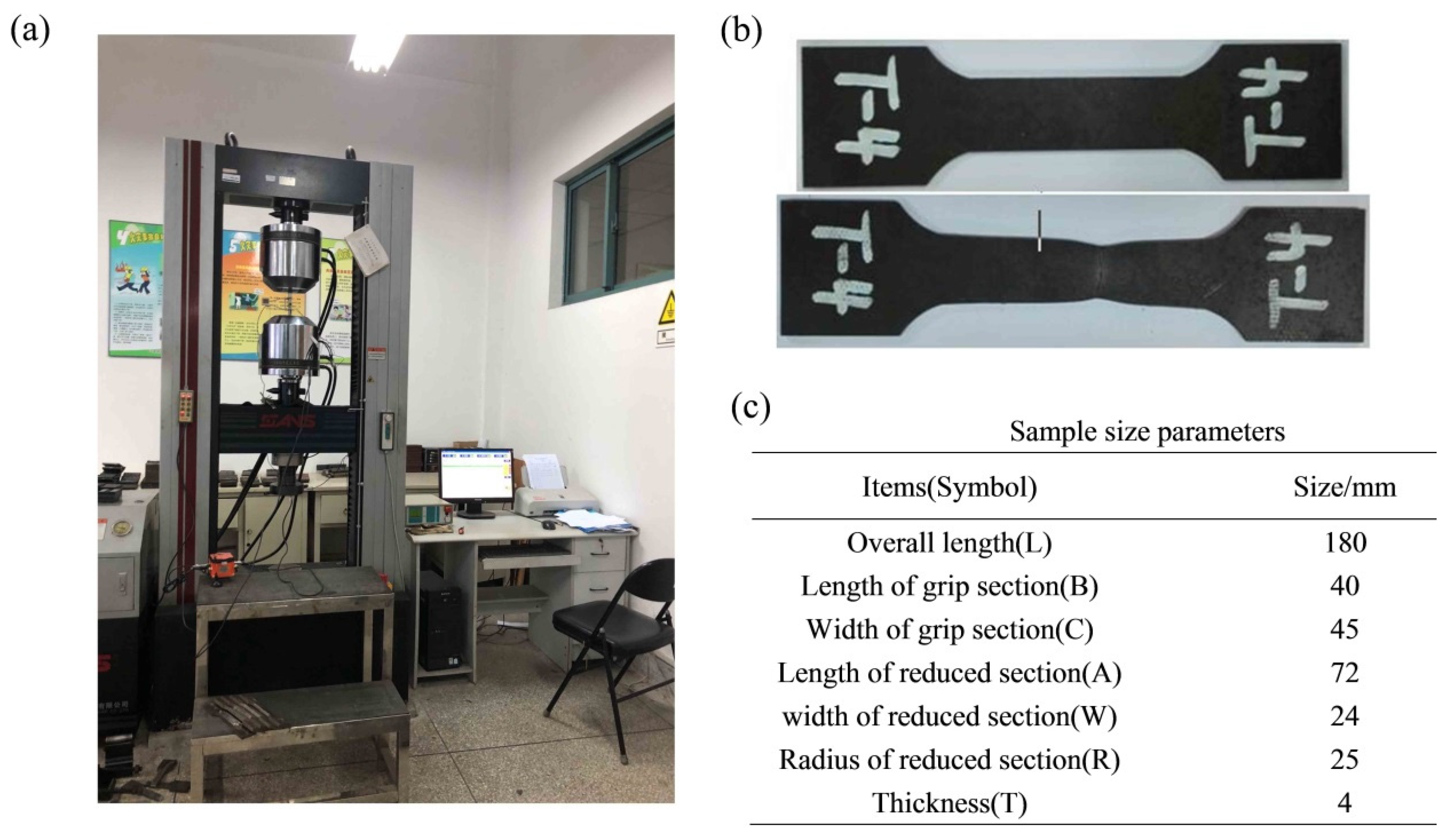
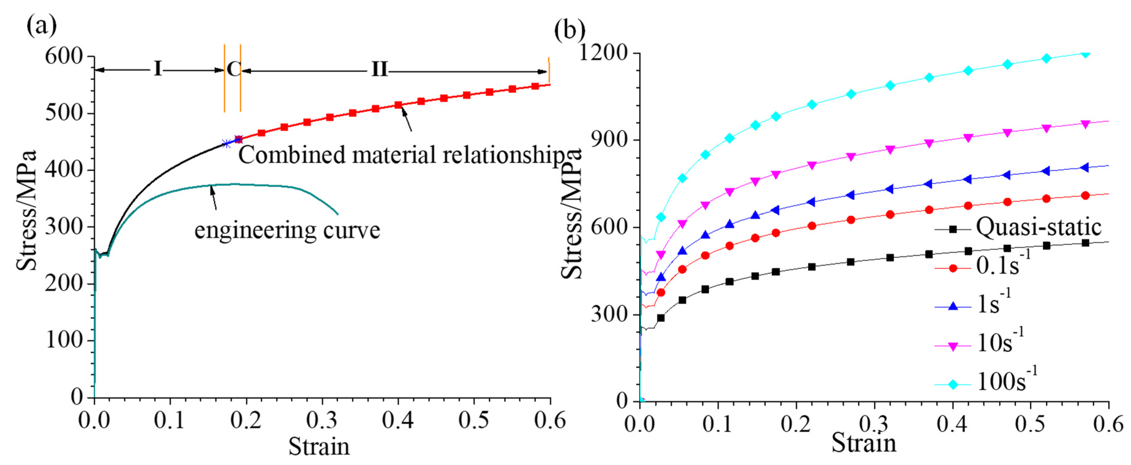
2.1. Quasi-Static Tensile Tests
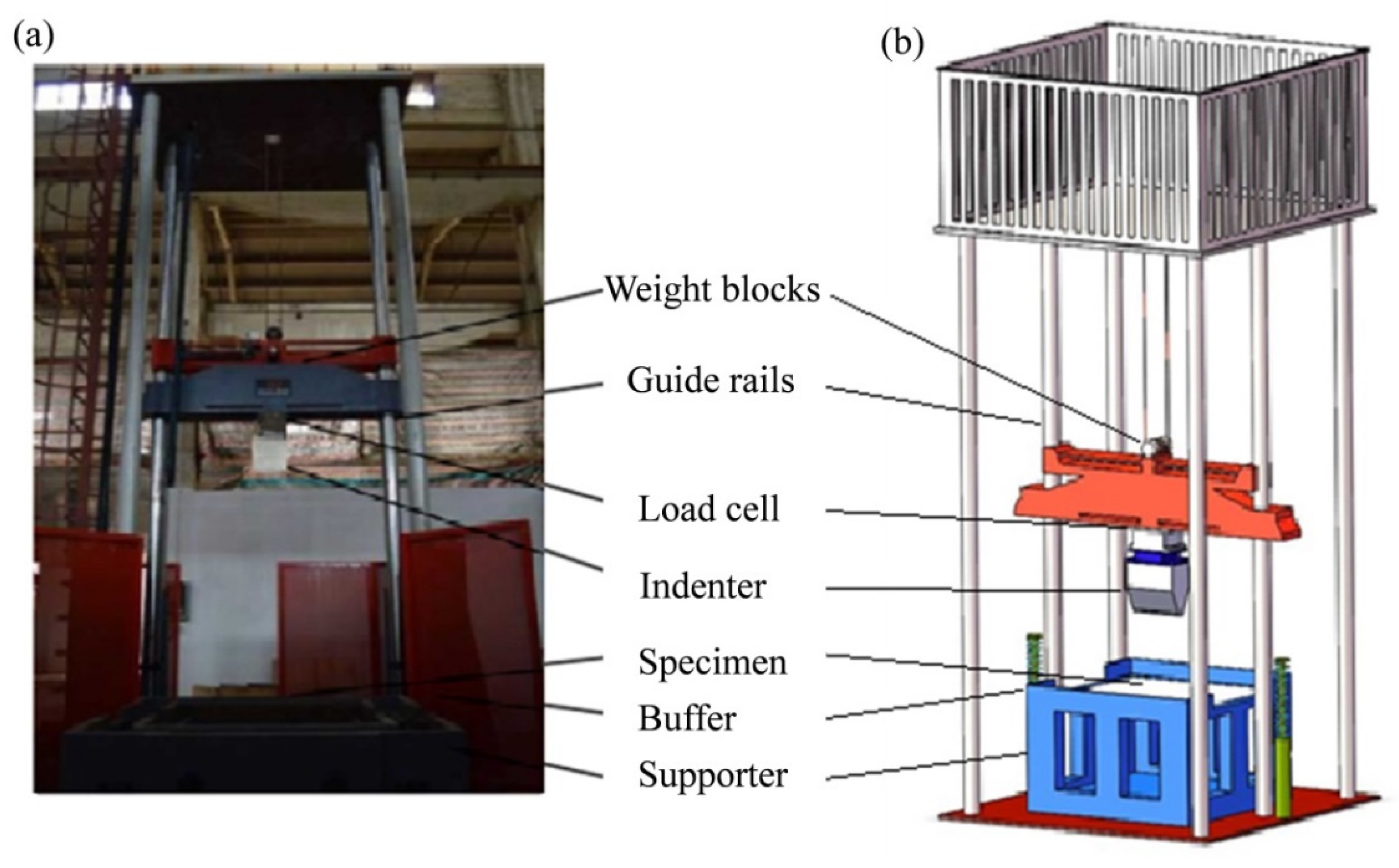
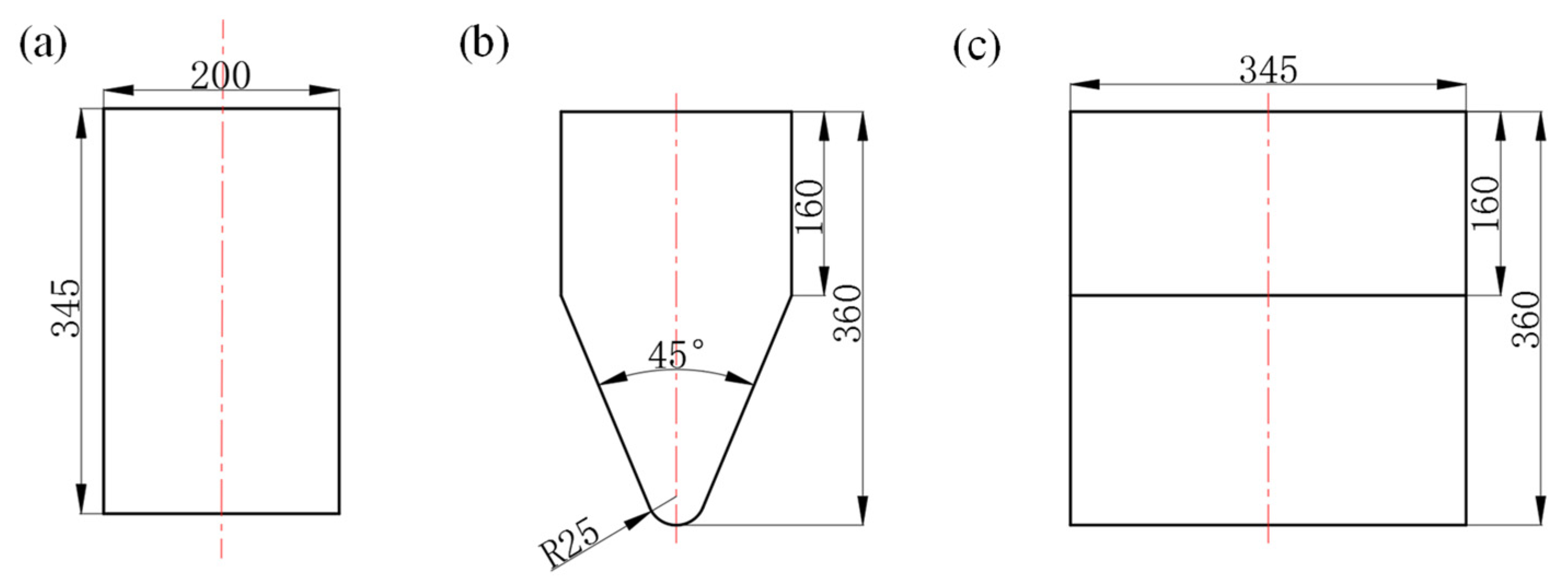
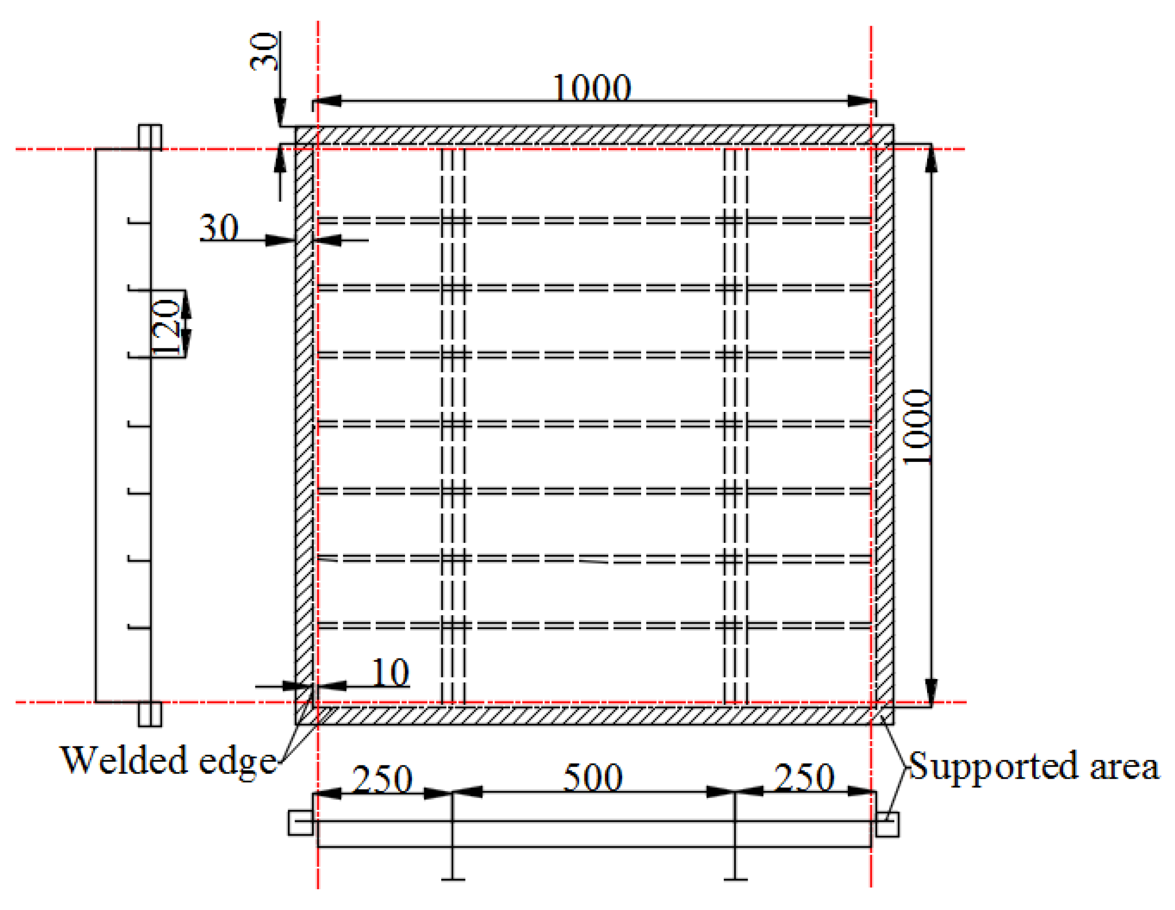
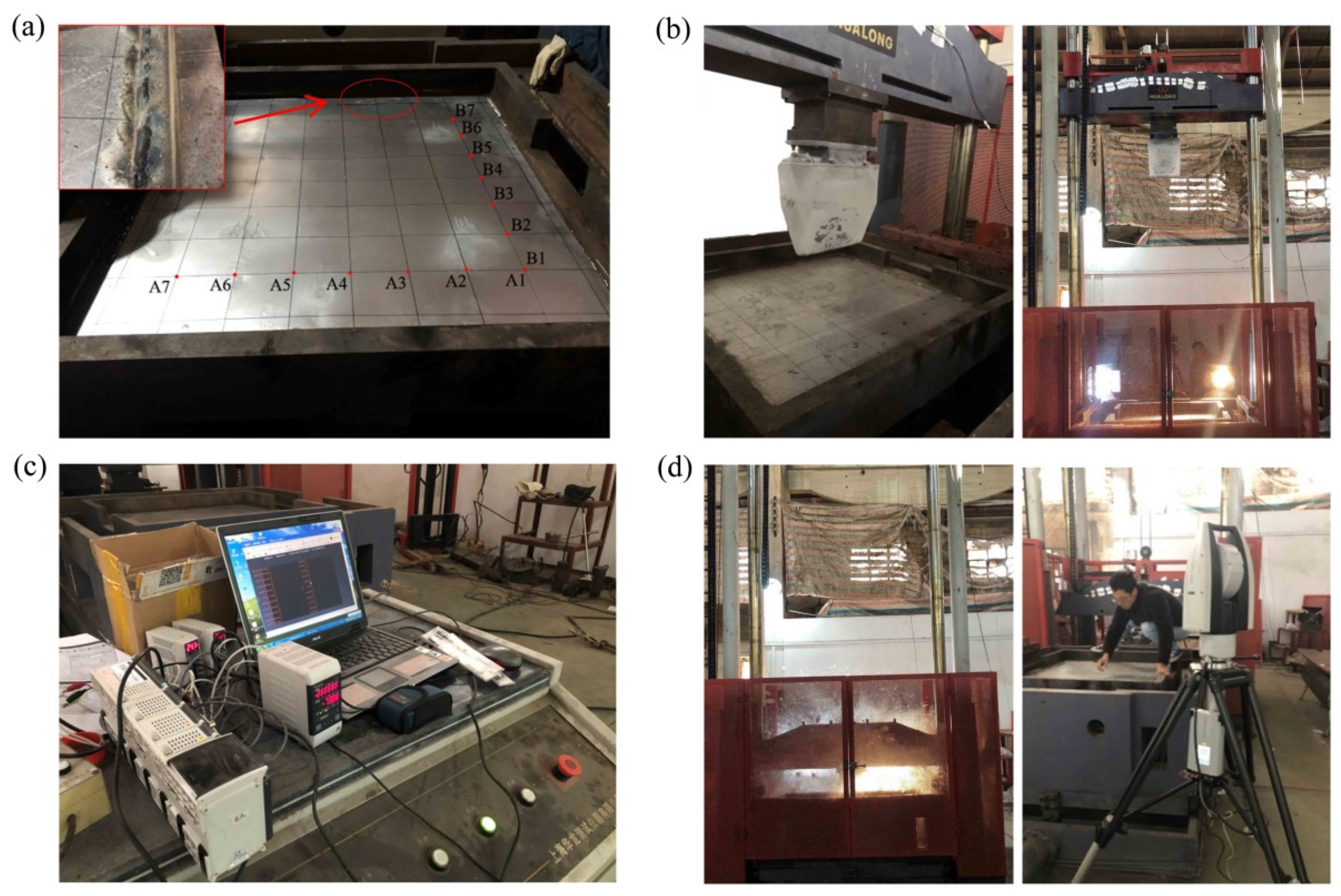
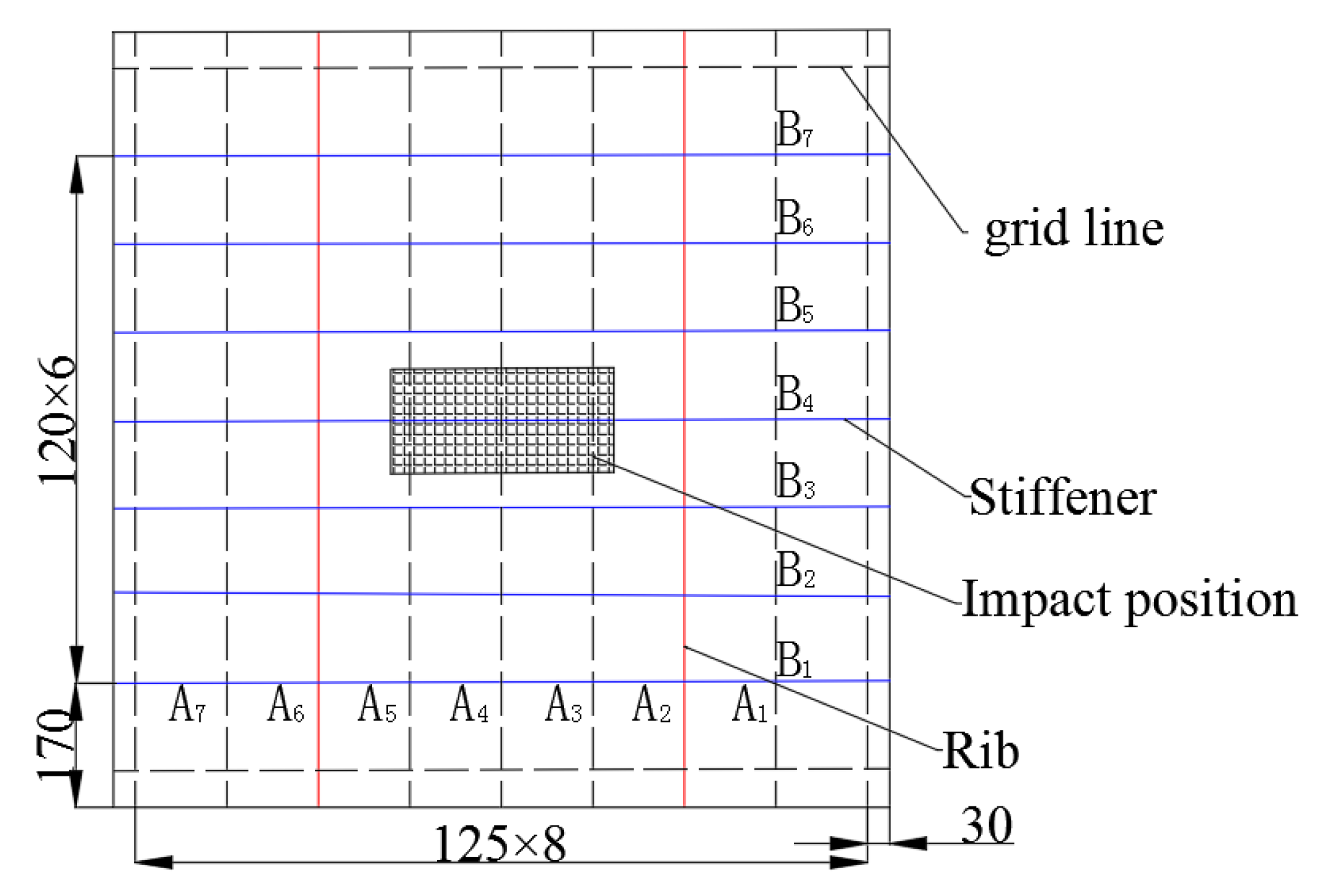
2.2. Impact Test of Stiffened Panel Struck by an Ice Indenter
2.3. Experimental Results
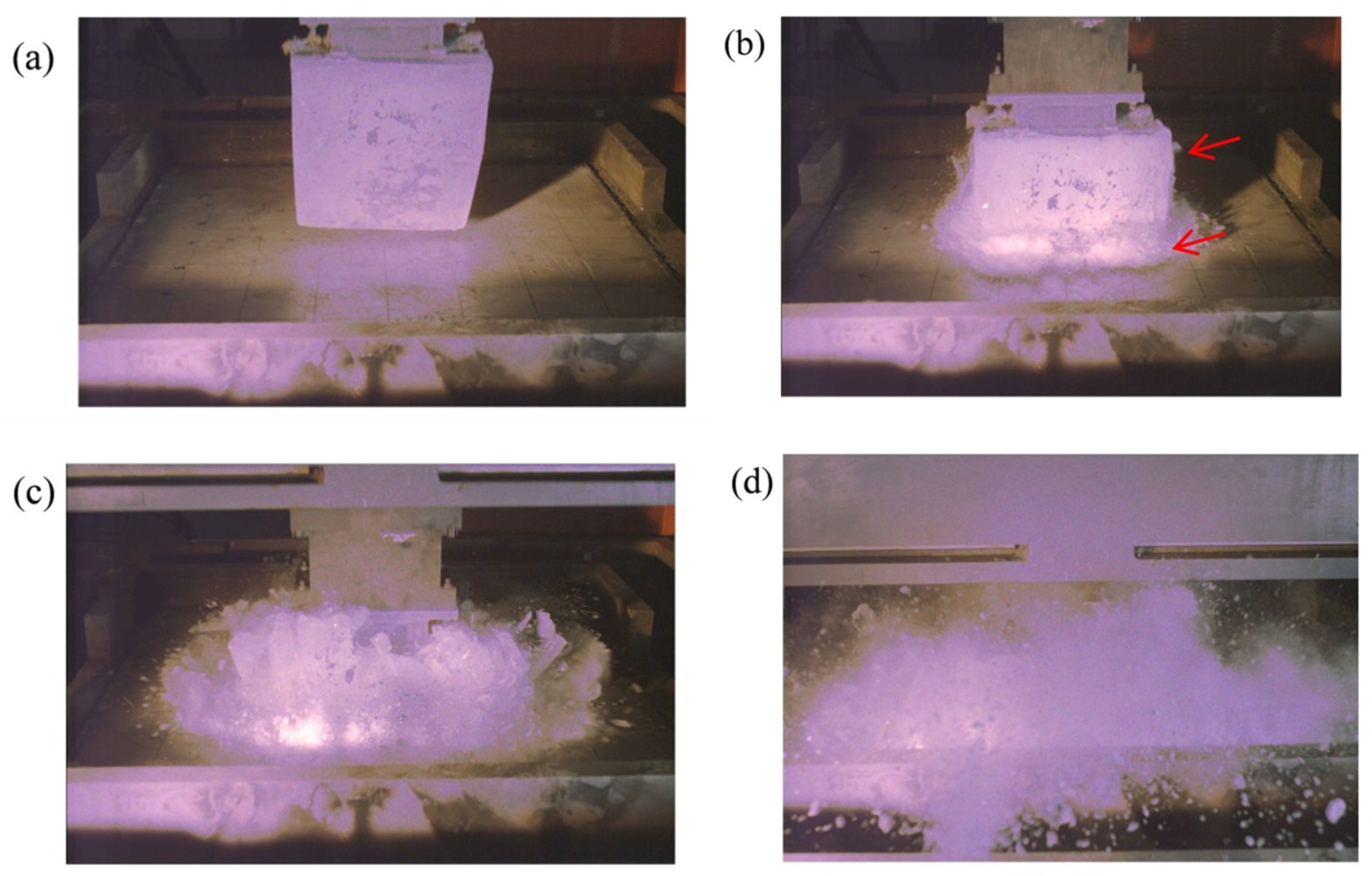
2.3.1. Ice Damage
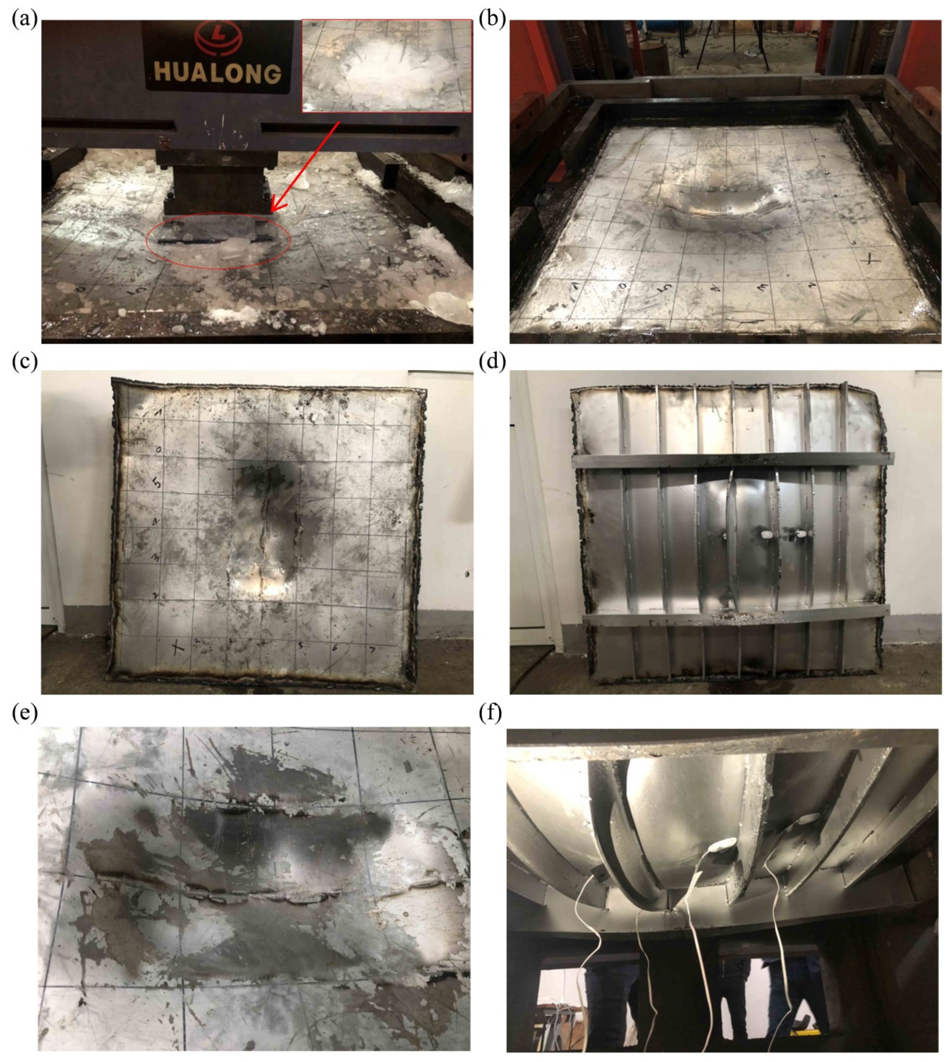
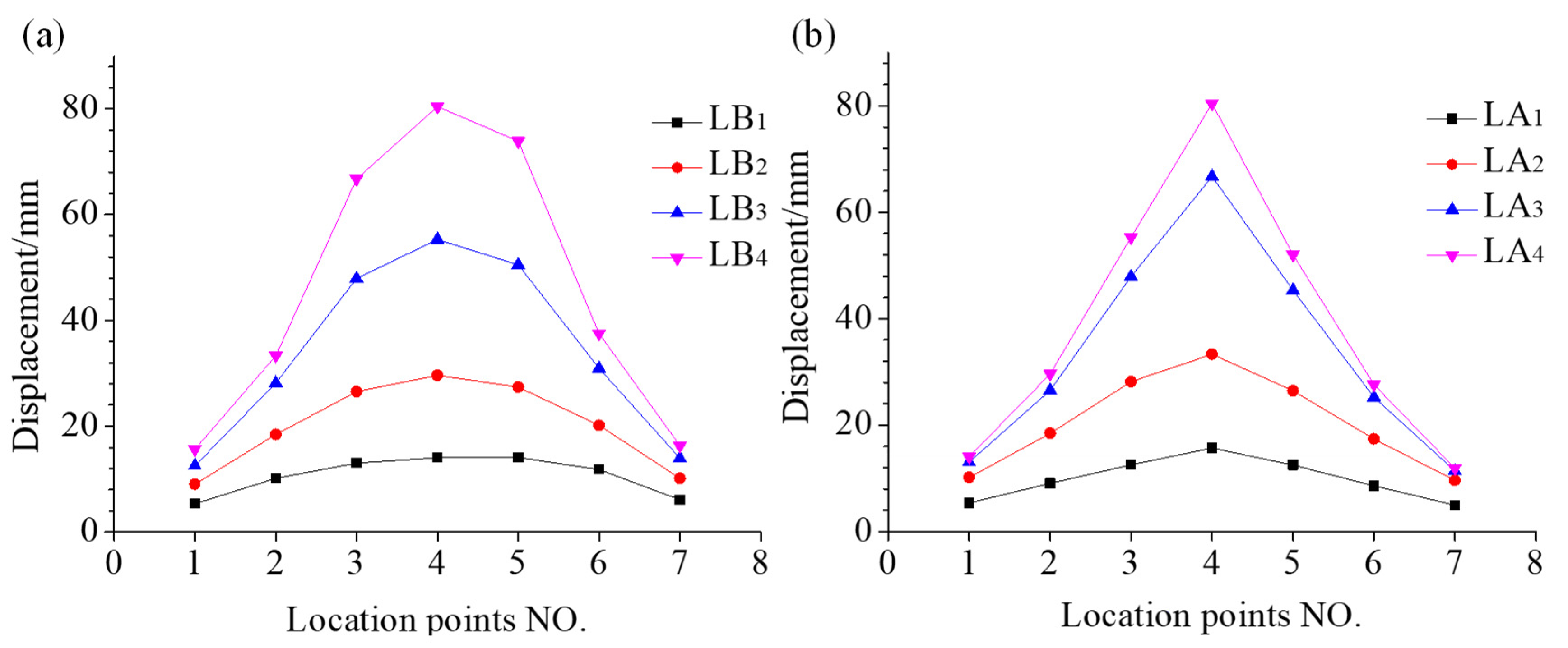
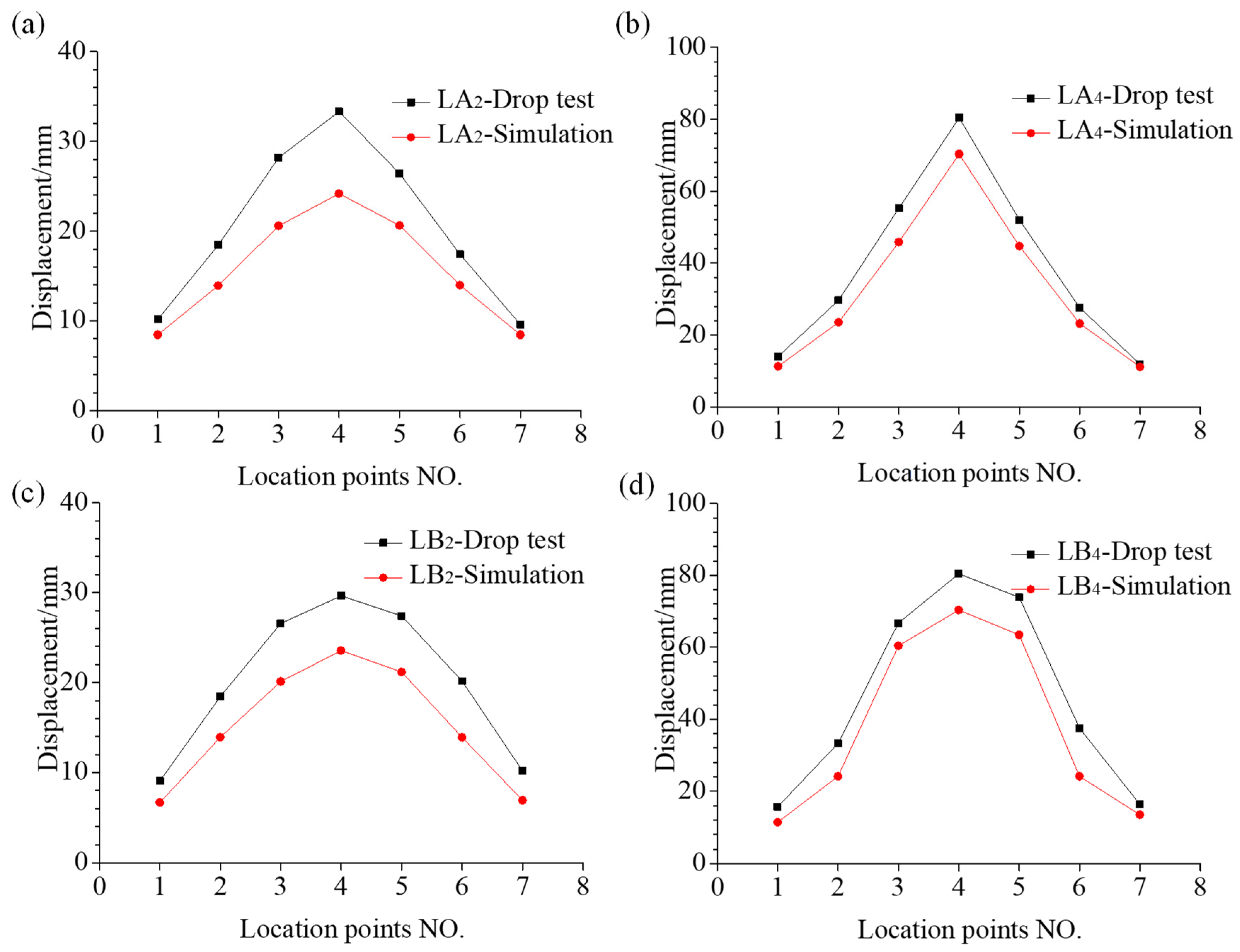
2.3.2. Structural Deformation
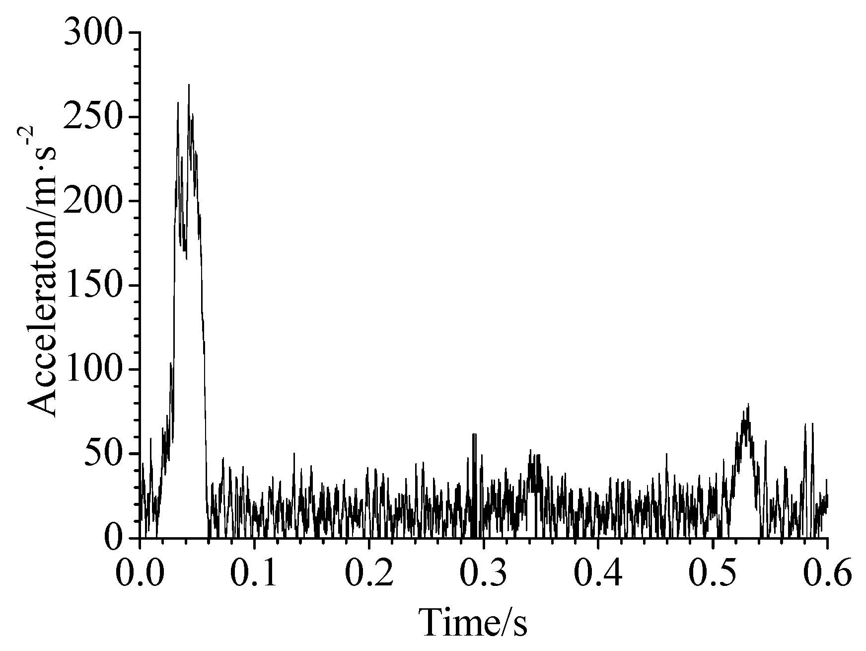
2.3.3. Acceleration Response
3. Numerical Simulation
3.1. Ice Material Model
3.1.1. Constitutive Model
3.1.2. Stress Update Algorithm
3.1.3. Calibration of the Material Model
3.2. Simulation Details
3.2.1. True Stress-Strain Relationship
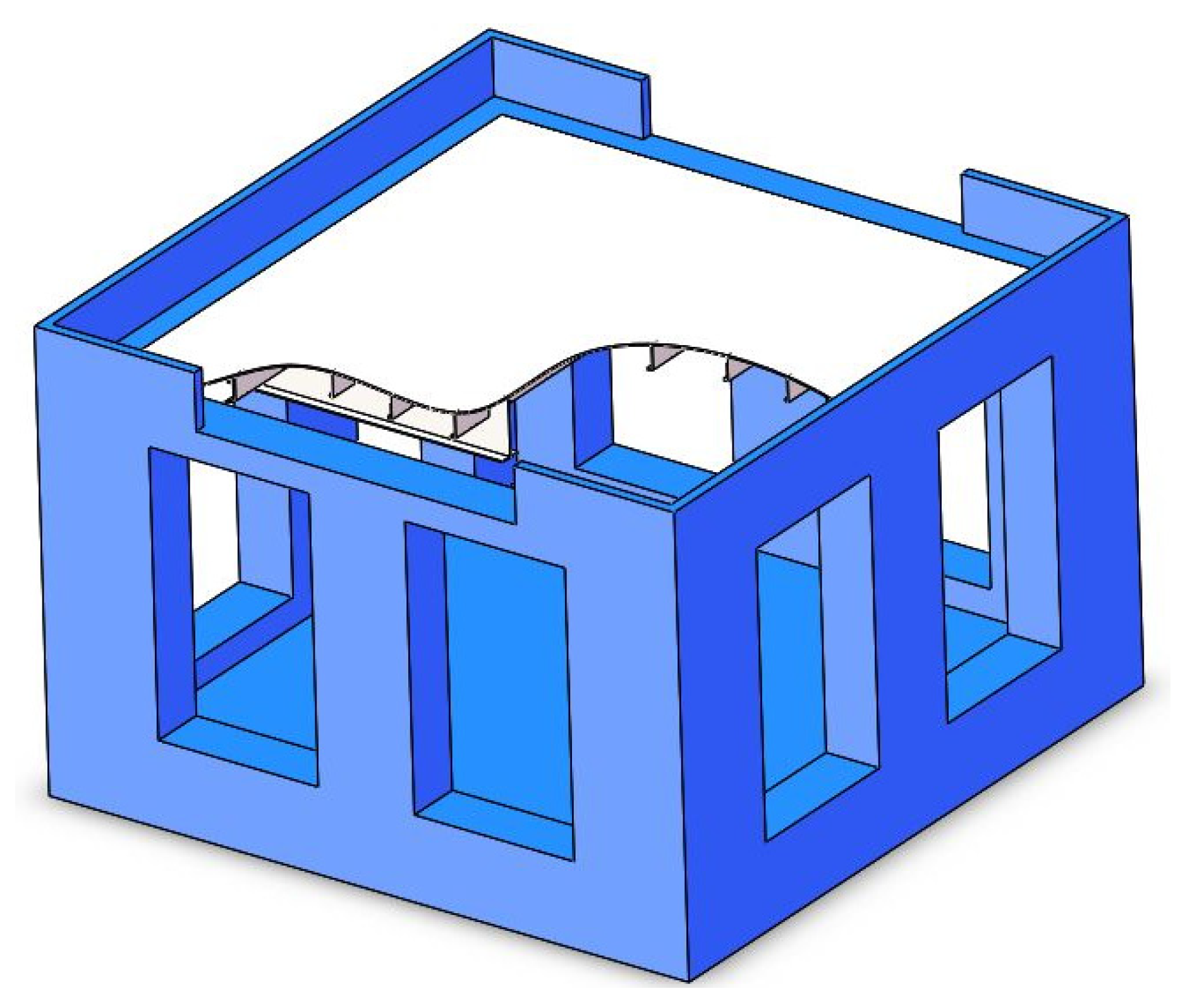
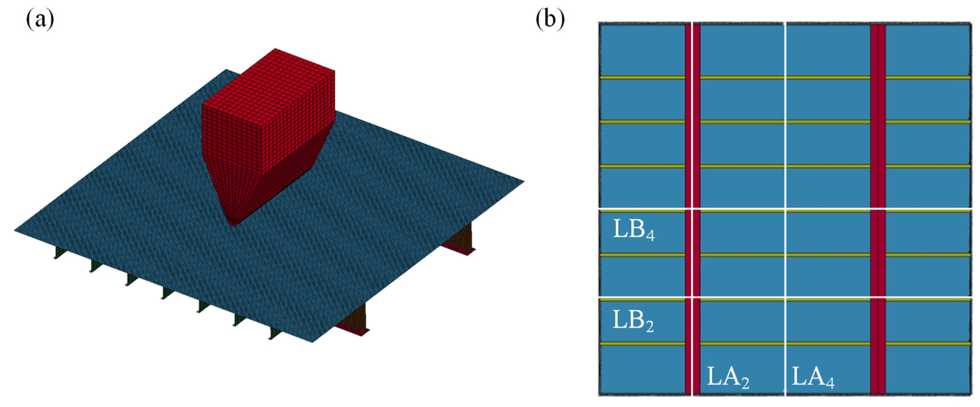
3.2.2. Finite Element Model
3.3. Simulation Results
4. Discussions
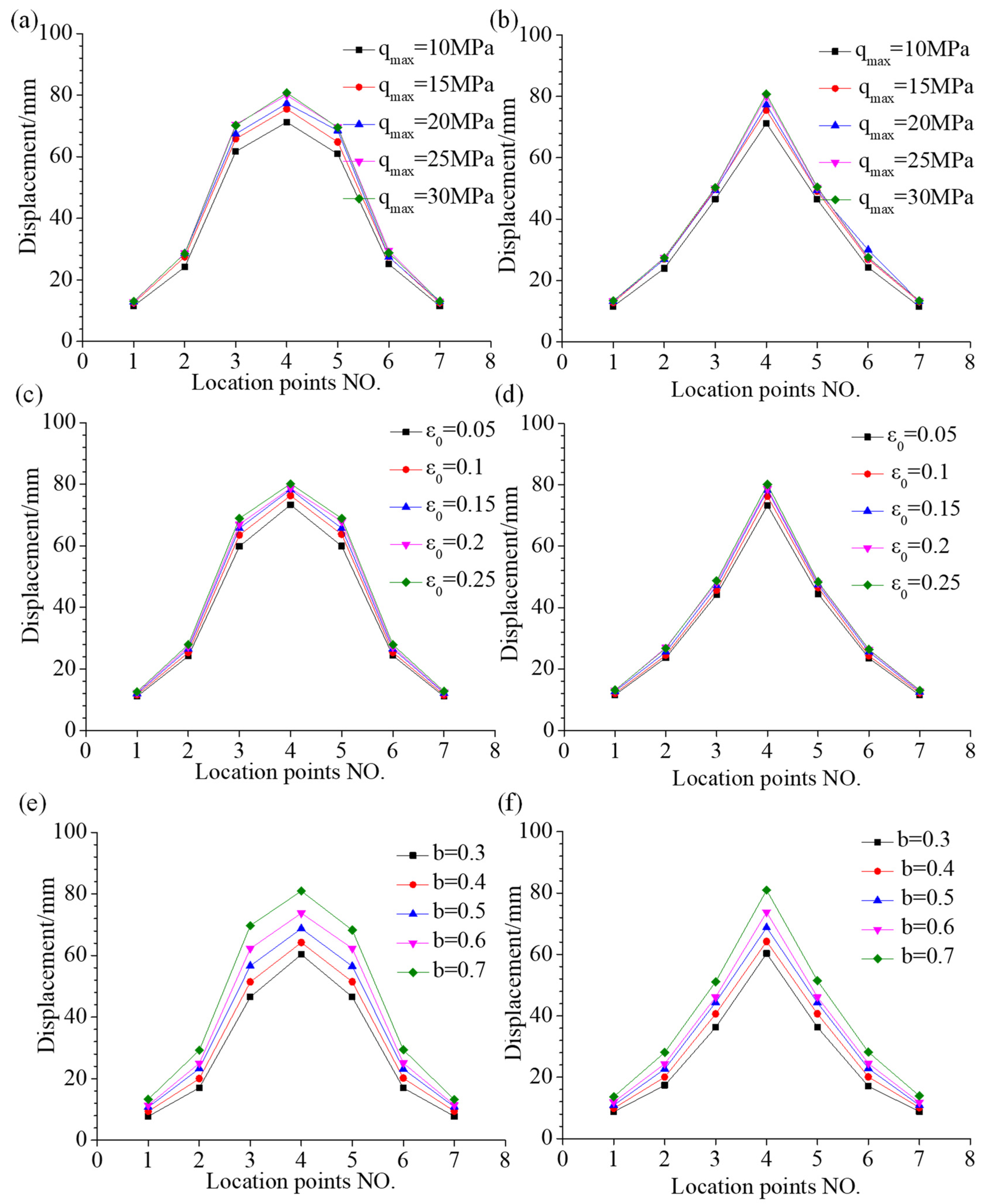
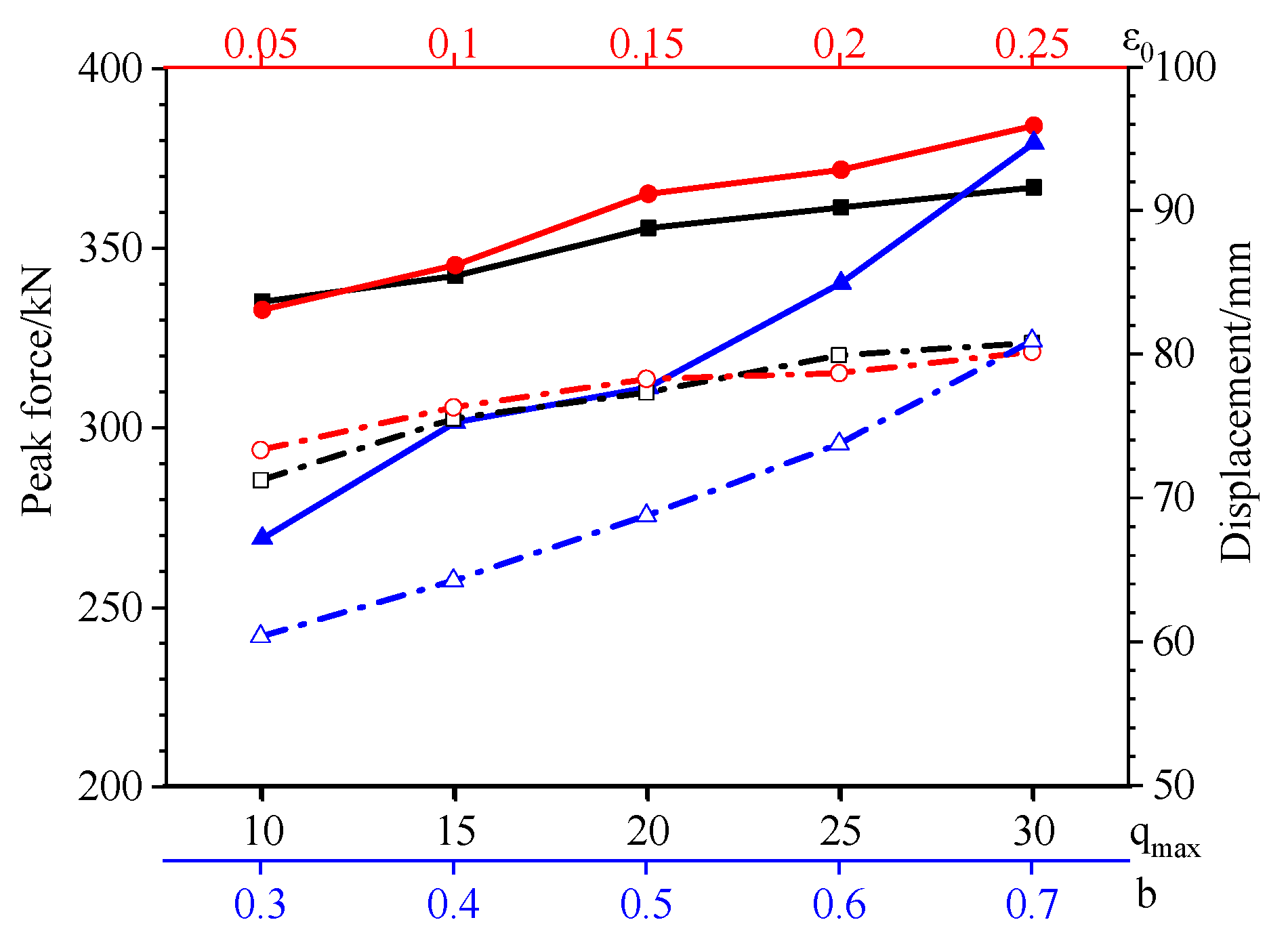
4.1. Effect of Parameters , , and
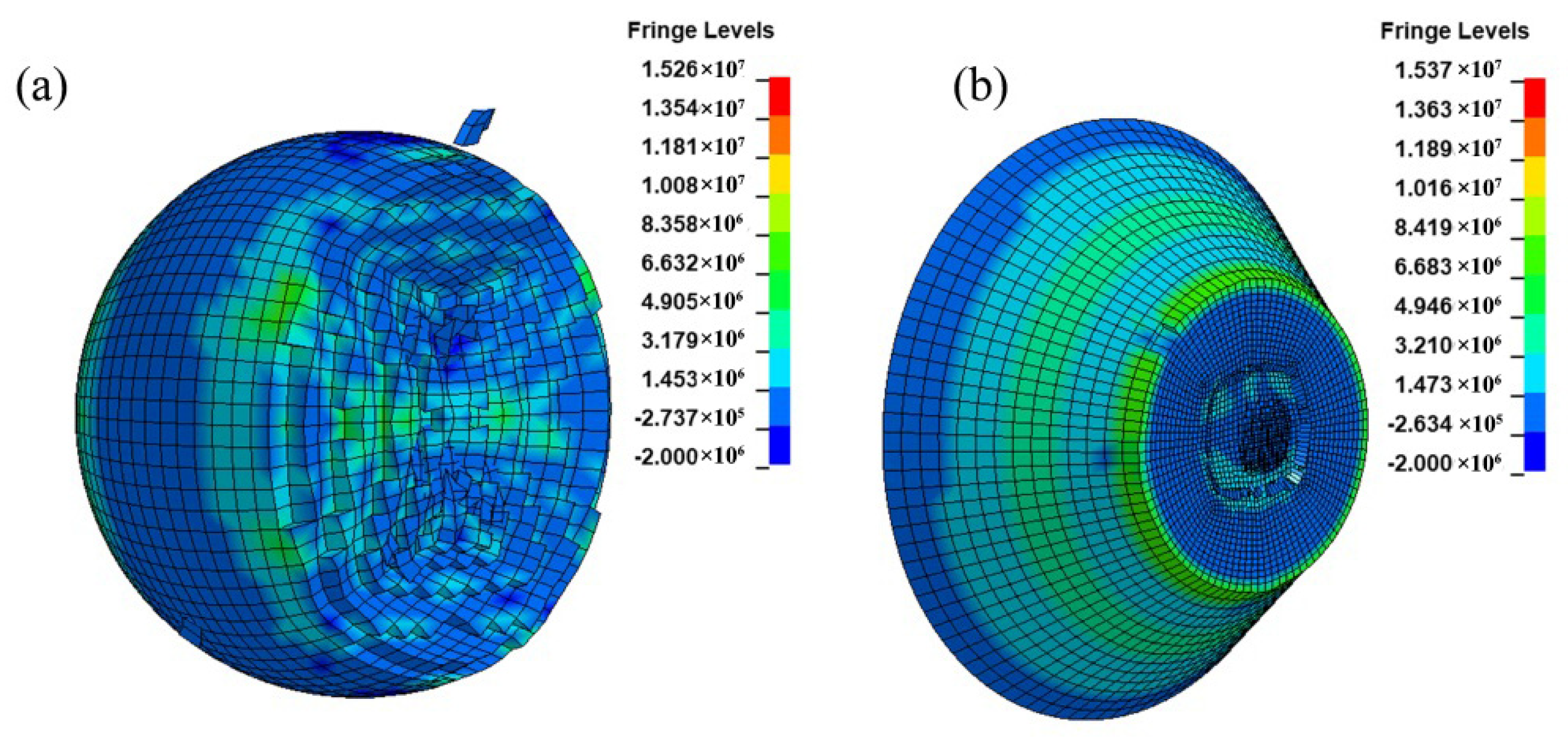
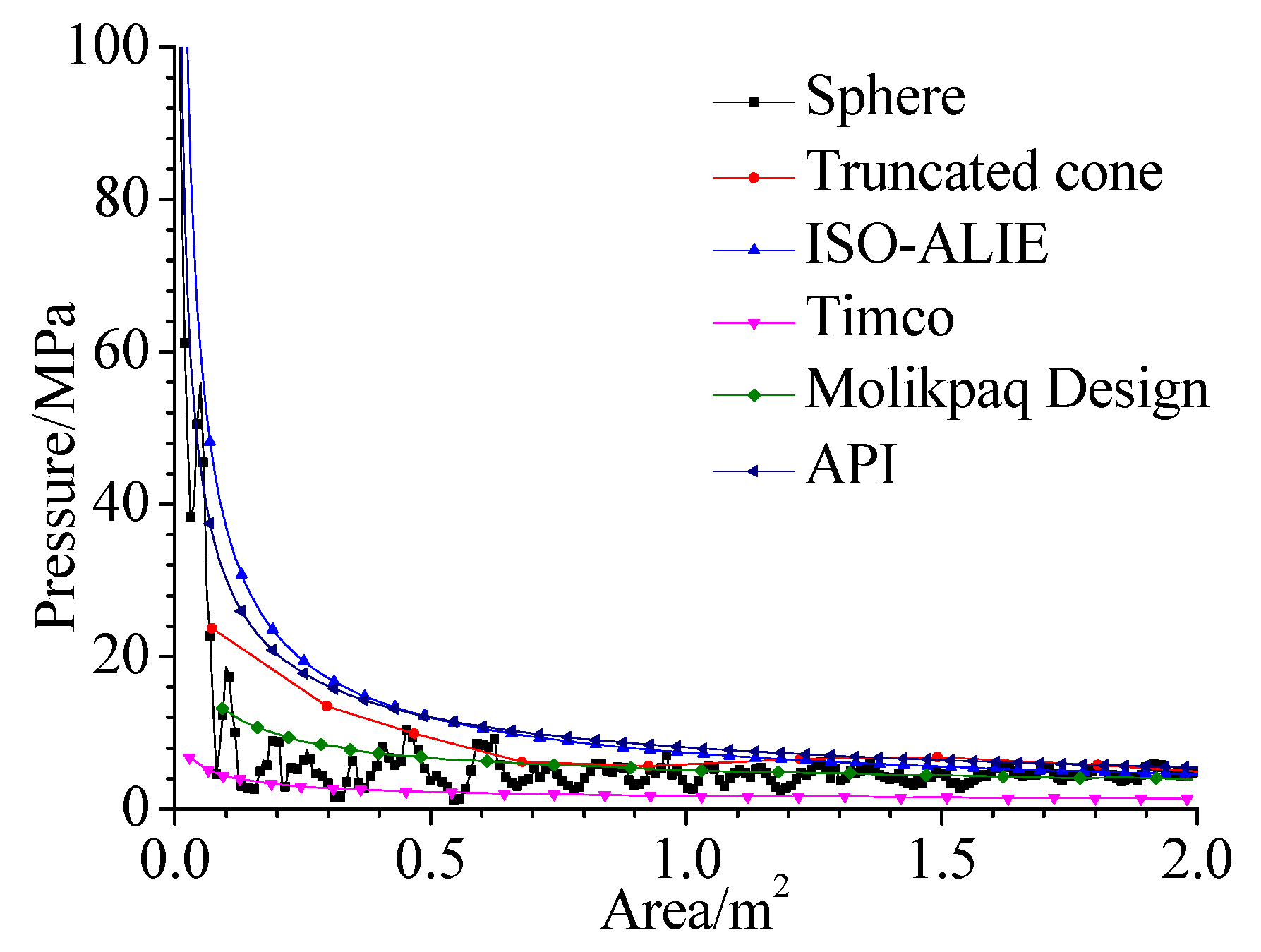
4.2. Comparison with Other Ice Material Models
5. Conclusions
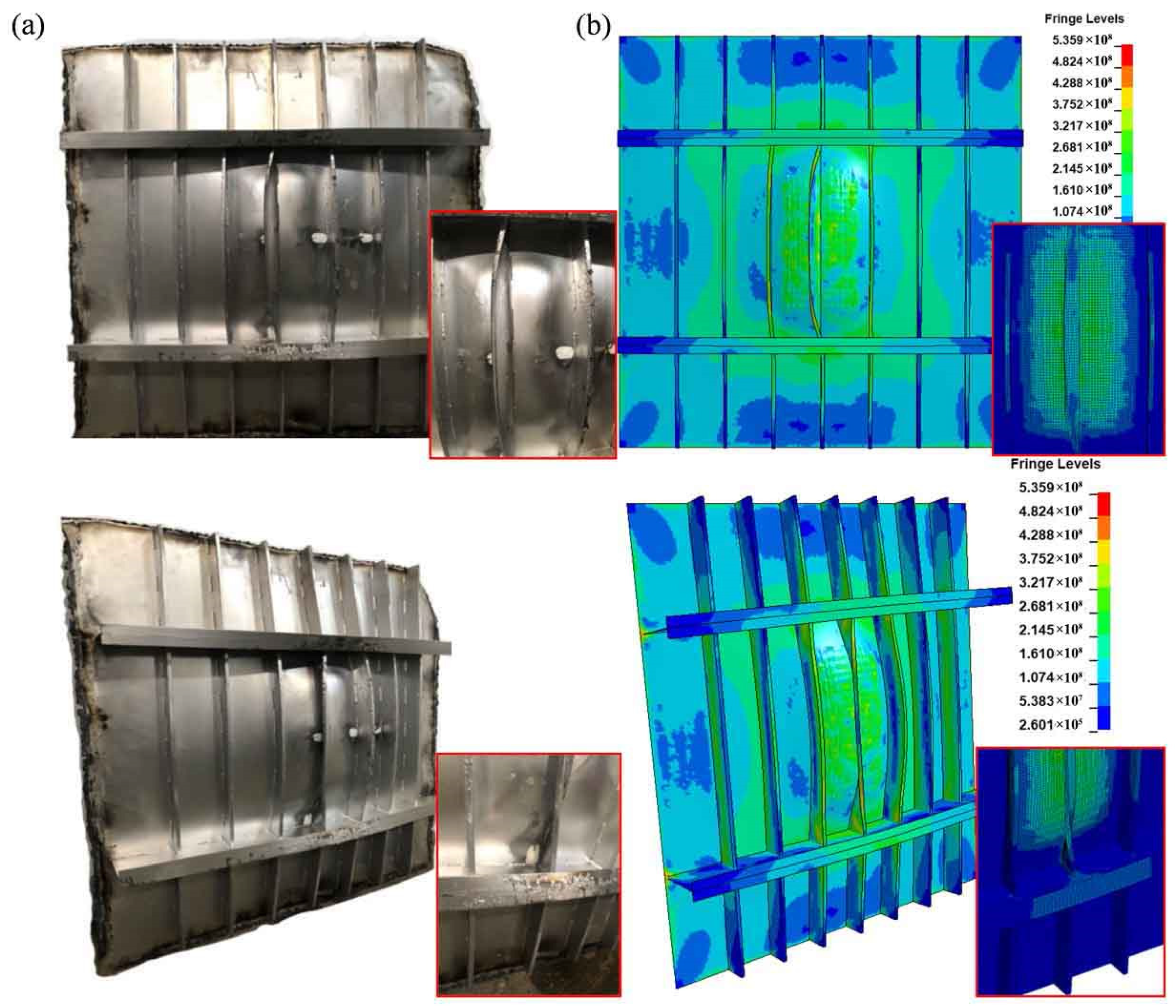
- The impact test shows that the ice indenter caused a significant indentation and experienced severe crushing and scattering. No obvious destruction or structural failure occurs. The deformation is localized at the impact area, and the main supporting components suffer substantial buckling deformation. The crushed ice was tightly compressed in the depression and experienced three-dimension stress state, which plays an important role in the structure’s deformation.
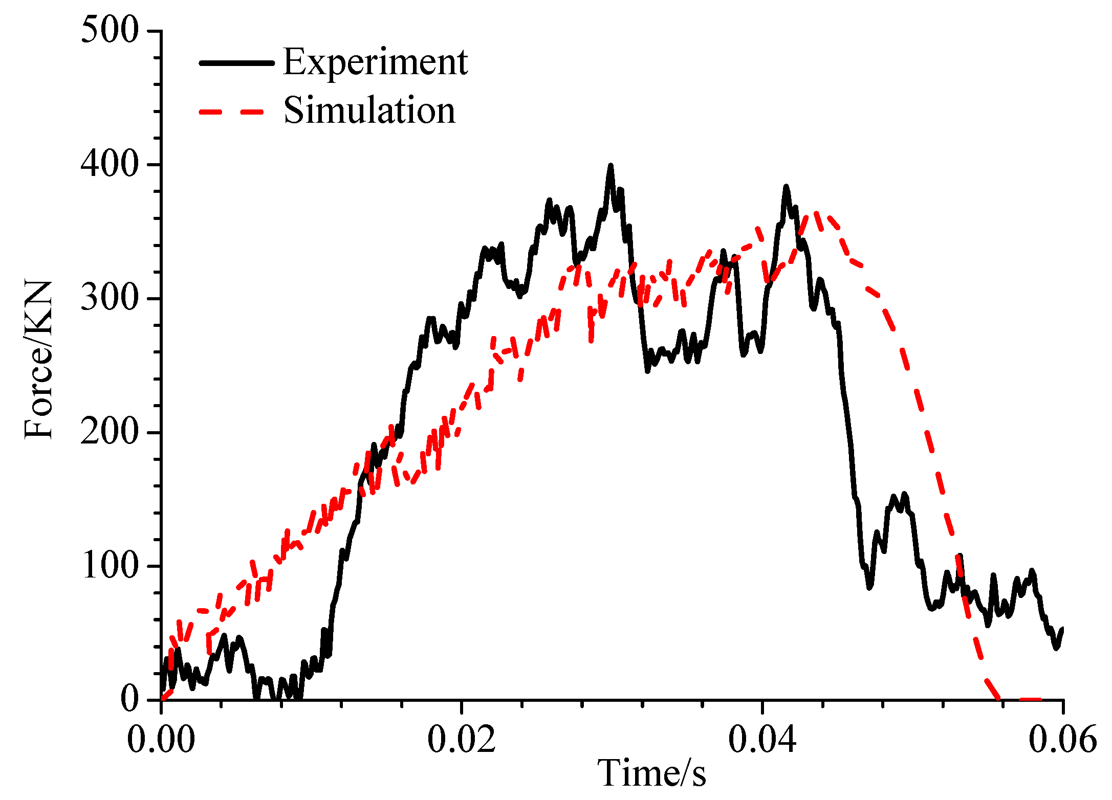
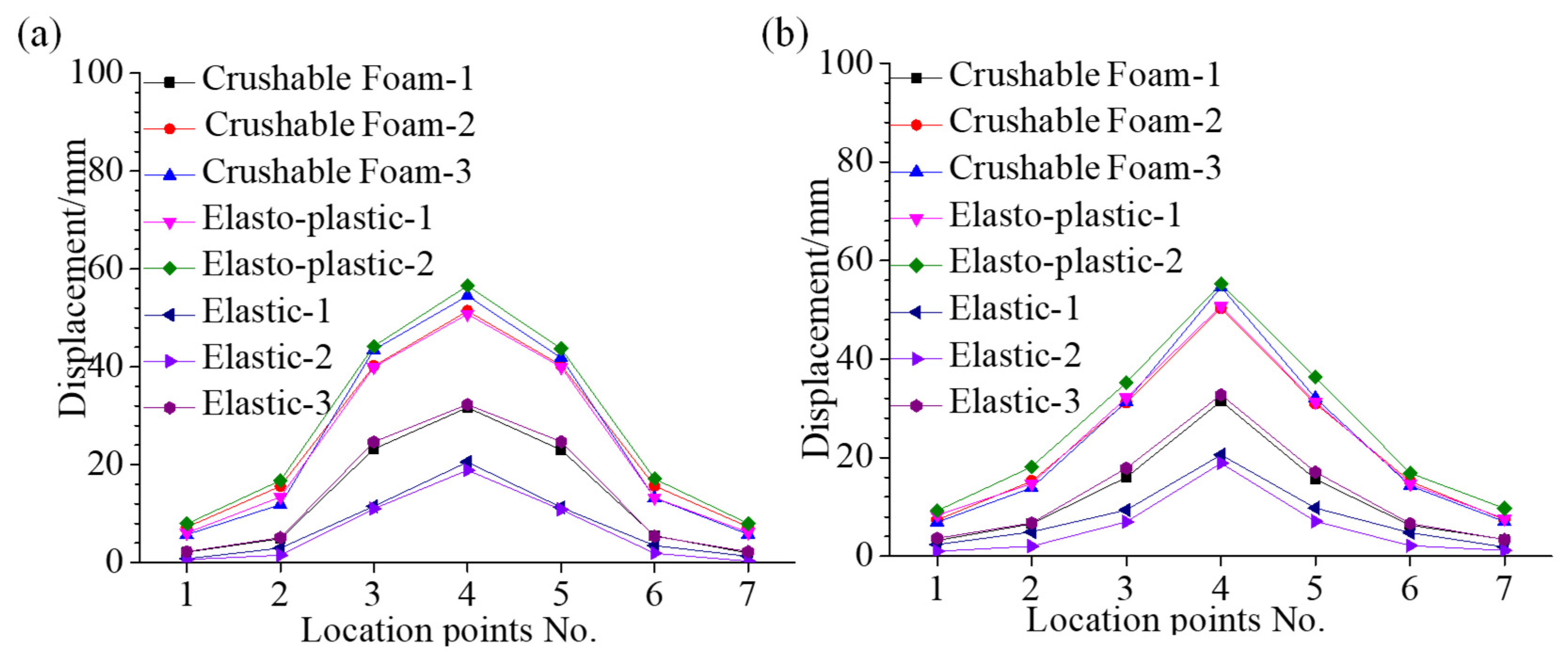
- The elasto-plastic constitutive model based on the multisurface yield envelope and empirical failure criterion is successfully applied. A similar deformation mode is observed, and the deformation of stiffeners and ribs is captured accurately. The relative errors are approximately 12.03% and 14.30% for the deformation and peak force, respectively.
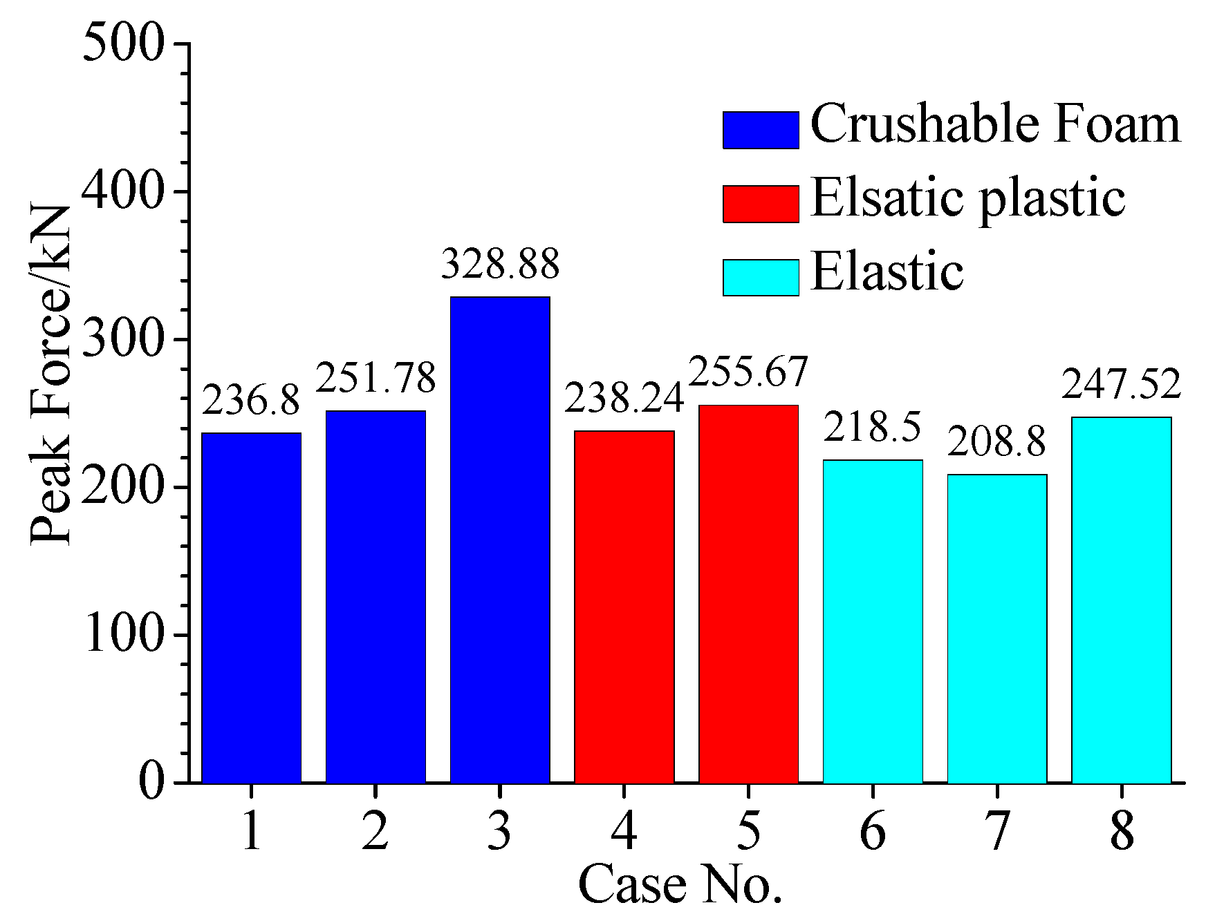
- According to the sensitivity study, the stiffened panel increases in both peak force and deformation with increasing values of parameters , , and , and the values of has the greatest degree of influence. Compared to other ice materials, the elasto-plastic material exhibited the best performance. It is confirmed that a reasonable and meaningful yield equation and failure criterion are both significant and indispensable.
Author Contributions
Funding
Data Availability Statement
Conflicts of Interest
References
- Hill, B.T. Ship collision with iceberg database. In Proceedings of the 7th International Conference and Exhibition on Performance of Ships and Structures in Ice, Banff, AB, Canada, 16–19 July 2006; pp. 16–19. [Google Scholar]
- Hänninen, S. Incidents and Accidents in Winter Navigation in the Baltic Sea, Winter 2002–2003; Finnish Maritime Administration: Helsinki, Finland, 2005. [Google Scholar]
- ISO 19906; Petroleum and Natural Gas Industries–Arctic Offshore Structures. International Standardization Organization: Geneva, Switzerland, 2010.
- Huang, Y.; Sun, J.; Ji, S.; Tian, Y. Experimental study on the resistance of a transport ship navigating in level ice. J. Mar. Sci. Appl. 2016, 15, 105–111. [Google Scholar] [CrossRef]
- Wang, C.; Hu, X.; Tian, T.; Guo, C. Numerical simulation of ice loads on a ship in broken ice fields using an elastic ice model. Int. J. Nav. Arch. Ocean Eng. 2020, 12, 414–427. [Google Scholar] [CrossRef]
- Ince, S.T.; Kumar, A.; Park, D.K.; Paik, J.K. An advanced technology for structural crashworthiness analysis of a ship colliding with an ice-ridge: Numerical modelling and experiments. Int. J. Impact Eng. 2017, 110, 112–122. [Google Scholar] [CrossRef]
- NORSOK. Design of Steel Structures. Appendix A: Design against Accidental Actions; Standards Norway: Oslo, Norway, 2004; p. 88. [Google Scholar]
- Schwarz, J.; Weeks, W.F. Engineering properties of sea ice. J. Glaciol. 1977, 19, 499–531. [Google Scholar] [CrossRef] [Green Version]
- Hutchings, J.K.; Heil, P.; LeComte, O.; Stevens, R.; Steer, A.; Lieser, J.L. Comparing methods of measuring sea-ice density in the East Antarctic. Ann. Glaciol. 2015, 56, 77–82. [Google Scholar] [CrossRef] [Green Version]
- Forsström, S.; Gerland, S.; Pedersen, C.A. Thickness and density of snow-covered sea ice and hydrostatic equilibrium as-sumption from in situ measurements in Fram Strait, the Barents Sea and the Svalbard coast. Ann. Glaciol. 2011, 52, 261–270. [Google Scholar] [CrossRef] [Green Version]
- Timco, G.; Frederking, R.M.W. A review of sea ice density. Cold Reg. Sci. Technol. 1996, 24, 1–6. [Google Scholar] [CrossRef]
- Sodhi, D.S.; Haehnel, R.B. Crushing Ice Forces on Structures. J. Cold Reg. Eng. 2003, 17, 153–170. [Google Scholar] [CrossRef]
- Daley, C.G. Energy based ice collision forces. In Proceedings of the 15th International Conference on Port and Ocean Engi-neering under Arctic Conditions (POAC), Espoo, Finland, 23–27 August 1999; pp. 674–686. [Google Scholar]
- Kujala, P. Semi-empirical evaluation of long term ice loads on a ship hull. Mar. Struct. 1996, 9, 849–871. [Google Scholar] [CrossRef]
- Hibler, W.D., III. A viscous sea ice law as a stochastic average of plasticity. J. Geophys. Res. Earth Surf. 1977, 82, 3932–3938. [Google Scholar] [CrossRef]
- Hibler, W.D., III. A Dynamic Thermodynamic Sea Ice Model. J. Phys. Oceanogr. 1979, 9, 815–846. [Google Scholar] [CrossRef] [Green Version]
- Carney, K.S.; Benson, D.J.; Bois, P.D.; Lee, R. A high strain rate model with failure for ice in LS-DYNA. In Proceedings of the 9th International LS-DYNE Users Conference, Detroit, MI, USA, 12–14 June 2006; pp. 1–15. [Google Scholar]
- Gagnon, R.E.; Derradji-Aouat, A. First results of numerical simulations of bergy bit collisions with the CCGS terry fox icebreaker. In Proceedings of the 18th IAHR International Symposium on Ice, Sapporo, Japan, 28 August–1 September 2006; pp. 9–16. [Google Scholar]
- Gagnon, R.E. A numerical model of ice crushing using a foam analogue. Cold Reg. Sci. Technol. 2011, 65, 335–350. [Google Scholar] [CrossRef] [Green Version]
- Gratz, E.T. Brittle Failure of Columnar S2 Ice under Triaxial Compression; Dartmouth College: Hanover, NH, USA, 1996; pp. 40–55. [Google Scholar]
- Cox, G.F.; Richter-Menge, J.A. Triaxial compression testing of ice. In Civil Engineering in the Arctic Offshore; American Society of Civil Engineers: San Francisco, CA, USA, 1985; pp. 476–488. [Google Scholar]
- Richter-Menge, J.A. Triaxial Testing of First-Year Sea Ice; US Army Corps of Engineers, Cold Regions Research & Engineering Laboratory: Hanover, NH, USA, 1986. [Google Scholar]
- Gagnon, R.E.; Gammon, P.H. Triaxial experiments on iceberg and glacier ice. J. Glaciol. 1995, 41, 528–540. [Google Scholar] [CrossRef] [Green Version]
- Jones, S.J. The confined compressive strength of polycrystalline ice. J. Glaciol. 1982, 28, 171–178. [Google Scholar] [CrossRef] [Green Version]
- Liu, Z.; Amdahl, J.; Løset, S. Plasticity based material modelling of ice and its application to ship–iceberg impacts. Cold Reg. Sci. Technol. 2011, 65, 326–334. [Google Scholar] [CrossRef]
- Gao, Y.; Hu, Z.; Ringsberg, J.W.; Wang, J. An elastic—Plastic ice material model for ship-iceberg collision simulations. Ocean Eng. 2015, 102, 27–39. [Google Scholar] [CrossRef]
- Shi, C.; Luo, Y.; Hu, Z. A Temperature-Gradient-Dependent Elastic-Plastic Material Model of Iceberg and its Application on the Simulation of FPSO-Iceberg Collision. In Proceedings of the 35th International Conference on Offshore Mechanics and Arctic Engineering, Busan, Korea, 19–24 June 2016; pp. 1–8. [Google Scholar]
- Shi, C.; Hu, Z.; Ringsberg, J.; Luo, Y. A nonlinear viscoelastic iceberg material model and its numerical validation. Proc. Inst. Mech. Eng. Part M J. Eng. Marit. Environ. 2017, 231, 675–689. [Google Scholar] [CrossRef] [Green Version]
- Wang, J.; Derradji-Aouat, A. Numerical prediction for resistance of Canadian icebreaker CCGS terry fox in level ice. In Proceedings of the International Conference on Ship and Offshore Technology, Busan, Korea, 10–11 December 2009; pp. 9–15. [Google Scholar]
- Ritch, R.; Frederking, R.; Johnston, M.; Browne, R.; Ralph, F. Local ice pressures measured on a strain gauge panel during the CCGS Terry Fox bergy bit impact study. Cold Reg. Sci. Technol. 2008, 52, 29–49. [Google Scholar] [CrossRef]
- Kim, E.; Storheim, M.; Amdahl, J.; Løset, S.; von Bock und Polach, R. Drop tests of ice blocks on stiffened panels with different structural flexibility. In Proceedings of the 6th International Conference on Collision and Grounding of Ships and Offshore Structures, Trondheim, Norway, 17–19 June 2013; pp. 241–250. [Google Scholar] [CrossRef]
- Kim, E.; Storheim, M.; Amdahl, J.; Løset, S.; von Bock und Polach, R.U.F. Laboratory experiments on shared-energy collisions between freshwater ice blocks and a floating steel structure. Ships Offshore Struct. 2017, 12, 530–544. [Google Scholar] [CrossRef] [Green Version]
- Storheim, M. Structural Response in Ship-Platform and Ship-Ice Collisions. Doctoral Thesis, Norwegian University of Science and Technology, Trondheim, Norway, January 2016. [Google Scholar]
- GB/T 228.1; Metallic Materials-Tensile Testing, Part I: Method of Test at Room Temperature. Standards Press of China: Beijing, China, 2010.
- Glen, J.W. The mechanical properties of ice I. The plastic properties of ice. Adv. Phys. 1958, 7, 254–265. [Google Scholar] [CrossRef]
- Derradji-Aouat, A. A unified failure envelope for isotropic fresh water ice and iceberg ice. In Proceedings of the ETCE/OMAE Joint Conference Energy for the New Millenium, New Orieans, LA, USA, 14–17 February 2000. [Google Scholar]
- Derradji-Aouat, A.A. Multi-surface failure criterion for saline ice in the brittle regime. Cold Reg. Sci. Technol. 2003, 36, 47–70. [Google Scholar] [CrossRef]
- Rist, M.A.; Murrell, S.A.F. Ice triaxial deformation and fracture. J. Glaciol. 1994, 40, 305–318. [Google Scholar] [CrossRef] [Green Version]
- Liu, Z. Analytical and Numerical Analysis of Iceberg Collisions with Ship Structures. Doctoral Thesis, Norwegian University of Science and Technology, Trondheim, Norway, 2011. [Google Scholar]
- Ralston, T.D. Yield and plastic deformation in ice crushing failure. In Proceedings of the ICSI/AIDJEX Symposium on Sea Ice-Processes and Models, Seattle, WA, USA, 6–9 September 1977. [Google Scholar]
- Jordaan, I.J.; Matskevitch, D.G.; Meglis, I.L. Disintegration of ice under fast compressive loading. Int. J. Fract. 1999, 97, 279–300. [Google Scholar] [CrossRef]
- Jones, S.J. High Strain-Rate Compression Tests on Ice. J. Phys. Chem. B 1997, 101, 6099–6101. [Google Scholar] [CrossRef]
- Ortiz, M.; Simo, J.C. An analysis of a new class of integration algorithms for elastoplastic constitutive relations. Int. J. Numer. Methods Eng. 1986, 23, 353–366. [Google Scholar] [CrossRef]
- Timco, G.W.; Johnston, M. Ice loads on the caisson structures in the Canadian Beaufort Sea. Cold Reg. Sci. Technol. 2004, 38, 185–209. [Google Scholar] [CrossRef]
- Timco, G.W.; Sudom, D. Revisiting the Sanderson pressure–area curve: Defining parameters that influence ice pressure. Cold Reg. Sci. Technol. 2013, 95, 53–66. [Google Scholar] [CrossRef]
- API Recommended Practice 2A-WSD. American Petroleum Institute Recommended Practice for Planning, Designing and Constructing Fixed Offshore Platforms—Working Stress Design; American Petroleum Institute: Washington, DC, USA, 2007. [Google Scholar]
- Villavicencio, R.; Guedes Soares, C. Numerical plastic response and failure of a pre-notched transversely impacted beam. Ships Offshore Struct. 2012, 7, 417–429. [Google Scholar] [CrossRef]
- Dieter, G.E. Mechanical behavior under tensile and compressive loads. ASM Handb. 2000, 8, 99–108. [Google Scholar] [CrossRef]
- Zhang, L.; Egge, E.D.; Bruhns, H. Approval Procedure Concept for Alternative Arrangements; Germanischer Lloyd: Hamburg, Germany, 2004; pp. 87–96. [Google Scholar]
- Jones, N. Structural Impact; Cambridge University Press: Cambridge, UK, 2011. [Google Scholar]
- Frederking, R.J.; Barker, A. Friction of sea ice on steel for condition of varying speeds. In Proceedings of the 20th International Offshore and Polar Engineering Conference, Kitakyushu, Japan, 26 May 2002; pp. 765–771. [Google Scholar]


| Items | Mild Steel | Ice Material | Units |
|---|---|---|---|
| Mass density | 7850 | 910 | kg/m3 |
| Elastic modulus | 209 | ≈2 | GPa |
| Poisson’s ratio | 0.3 | 0.3 | - |
| Yield stress | 265 | - | MPa |
| Ultimate tensile stress | 359 | - | MPa |
| Fracture strain | 0.29 | - | - |
| Items | Dimension and Thickness/mm |
|---|---|
| Plate | 2.5 |
| T bar | 100 × 2/40 × 2.5 |
| Stiffener | 42 × 1.75/8.5 × 3.3 |
| Impact Parameters | Values | Unit |
|---|---|---|
| Drop height | 3.2 | m |
| Impact weight | 1340 | kg |
| Impact velocity | 7.9 | m/s |
| Impact energy | 42.3 | kJ |
| Node ID | A1 | A2 | A3 | A4 | A5 | A6 | A7 |
|---|---|---|---|---|---|---|---|
| B1 | −5.36 | −10.15 | −13.02 | −14.07 | −14.11 | −11.85 | −6.12 |
| B2 | −9.07 | −18.45 | −26.56 | −29.64 | −27.39 | −20.16 | −10.18 |
| B3 | −12.55 | −28.17 | −47.92 | −55.29 | −50.50 | −30.96 | −13.96 |
| B4 | −15.69 | −33.32 | −66.73 | −80.43 | −73.85 | −37.52 | −16.35 |
| B5 | −12.50 | −26.42 | −45.35 | −52.04 | −46.89 | −28.92 | −13.71 |
| B6 | −8.61 | −17.41 | −25.21 | −27.60 | −25.62 | −18.57 | −9.74 |
| B7 | −4.94 | −9.60 | −11.37 | −11.89 | −11.66 | −10.37 | −5.85 |
| Items | ||||
| Values | 22.93 | 2.06 | −0.023 | 6.8 |
| Name | Expression |
|---|---|
| ISO-ALIE | |
| Molikpad Design [37] | |
| Timco [38] | |
| API [39] |
| Node ID | A1 | A2 | A3 | A4 | A5 | A6 | A7 |
|---|---|---|---|---|---|---|---|
| B1 | 4.511 | 8.452 | 10.394 | 11.272 | 10.294 | 8.449 | 4.775 |
| B2 | 6.678 | 13.943 | 20.121 | 23.552 | 21.161 | 13.900 | 6.931 |
| B3 | 9.637 | 20.584 | 36.372 | 45.849 | 38.208 | 20.607 | 9.913 |
| B4 | 11.412 | 24.179 | 60.389 | 70.751 | 63.422 | 24.184 | 13.468 |
| B5 | 9.609 | 20.640 | 36.246 | 44.736 | 37.452 | 20.699 | 9.613 |
| B6 | 7.564 | 13.986 | 20.284 | 23.227 | 20.271 | 14.032 | 6.696 |
| B7 | 4.221 | 8.450 | 10.471 | 11.154 | 10.384 | 8.487 | 4.513 |
| Cases | ||||||
|---|---|---|---|---|---|---|
| 1 | 49.58 | 4.46 | −0.049 | 10 | 0.05 | 0.3 |
| 2 | 111.57 | 10.04 | −0.112 | 15 | 0.1 | 0.4 |
| 3 | 198.35 | 17.85 | −0.198 | 20 | 0.15 | 0.5 |
| 4 | 309.92 | 27.89 | −0.309 | 25 | 0.2 | 0.6 |
| 5 | 446.28 | 40.17 | −0.446 | 30 | 0.25 | 0.7 |
| Cases No. | Case Name | MAT No. | Yield Criterion | Failure Criterion | Remarks |
|---|---|---|---|---|---|
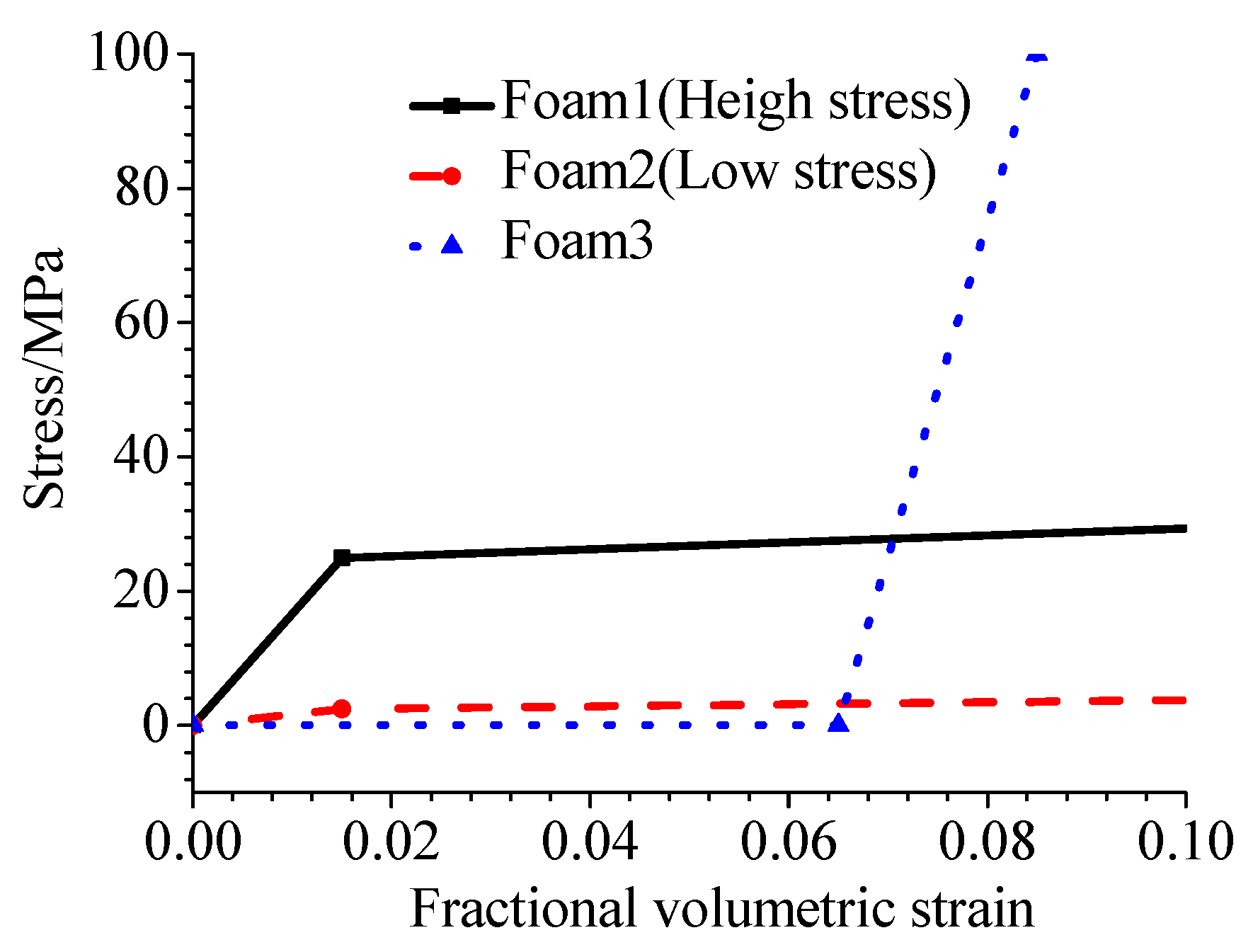
| 1 | Crushable Foam 1 | MAT 63 | 10 MPa | Figure 26, curve Foam 1 | |
| 2 | Crushable Foam 2 | MAT 63 | 10 MPa | Figure 26, curve Foam 2 | |
| 3 | Crushable Foam 3 | MAT 63 | 10 MPa | Figure 26, curve Foam 3 | |
| 4 | Elasto-plastic-1 | MAT 13 | 10 MPa | 0.01 | |
| 5 | Elasto-plastic-2 | MAT 13 | 20 MPa | 0.01 | |
| 6 | Elastic-1 | User defined | multisurface | ||
| 7 | Elastic-2 | MAT 1 | 10 MPa | ||
| 8 | Elastic-3 | MAT 1 | 20 MPa |
Publisher’s Note: MDPI stays neutral with regard to jurisdictional claims in published maps and institutional affiliations. |
© 2022 by the authors. Licensee MDPI, Basel, Switzerland. This article is an open access article distributed under the terms and conditions of the Creative Commons Attribution (CC BY) license (https://creativecommons.org/licenses/by/4.0/).
Share and Cite
Yu, T.; Wang, J.; Liu, J.; Liu, K. Experimental and Numerical Simulation of the Dynamic Response of a Stiffened Panel Suffering the Impact of an Ice Indenter. Metals 2022, 12, 505. https://doi.org/10.3390/met12030505
Yu T, Wang J, Liu J, Liu K. Experimental and Numerical Simulation of the Dynamic Response of a Stiffened Panel Suffering the Impact of an Ice Indenter. Metals. 2022; 12(3):505. https://doi.org/10.3390/met12030505
Chicago/Turabian StyleYu, Tongqiang, Jiaxia Wang, Junjie Liu, and Kun Liu. 2022. "Experimental and Numerical Simulation of the Dynamic Response of a Stiffened Panel Suffering the Impact of an Ice Indenter" Metals 12, no. 3: 505. https://doi.org/10.3390/met12030505