Least Squares Twin Support Vector Machines to Classify End-Point Phosphorus Content in BOF Steelmaking

Abstract

End-point phosphorus content in steel in a basic oxygen furnace (BOF) acts as an indicator of the quality of manufactured steel. An undesirable amount of phosphorus is removed from the steel by the process of dephosphorization. The degree of phosphorus removal is captured numerically by the ‘partition ratio’, given by the ratio of %wt phosphorus in slag and %wt phosphorus in steel. Due to the presence of multitudes of process variables, often, it is challenging to predict the partition ratio based on operating conditions. Herein, a robust data-driven classification technique of least squares twin support vector machines (LSTSVM) is applied to classify the ‘partition ratio’ to two categories (‘High’ and ‘Low’) steels indicating a greater or lesser degree of phosphorus removal, respectively. LSTSVM is a simpler, more robust, and faster alternative to the twin support vector machines (TWSVM) with respect to non-parallel hyperplanes-based binary classifications. The relationship between the ‘partition ratio’ and the chemical composition of slag and tapping temperatures is studied based on approximately 16,000 heats from two BOF plants. In our case, a relatively higher model accuracy is achieved, and LSTSVM performed 1.5–167 times faster than other applied algorithms.

1. Introduction

Production of high-quality steel using the basic oxygen furnace (BOF) requires a deep understanding of numerous complex chemical reactions and accurate end-point control [1]. In BOF, oxygen is blown into the liquid metal, which leads to a conversion of molten pig iron and scraps into liquid steel. Pig iron contains different types of impurities such as carbon, sulfur, manganese, and phosphorous. A high content of phosphorous in the final product leads to poor mechanical properties such as low ductility and increased brittleness, thus, increasing the probability of cracking during deformation and welding [2]. The process of removing phosphorous from pig iron to obtain high-quality steel in BOF is known as dephosphorization. In recent years, the phosphorous content in iron ores has increased significantly, making the dephosphorization process more critical [3]. Research has shown that for a given basicity and carbon content, the presence of iron oxide has a greater effect on dephosphorization compared to dissolved oxygen in steel [4]. 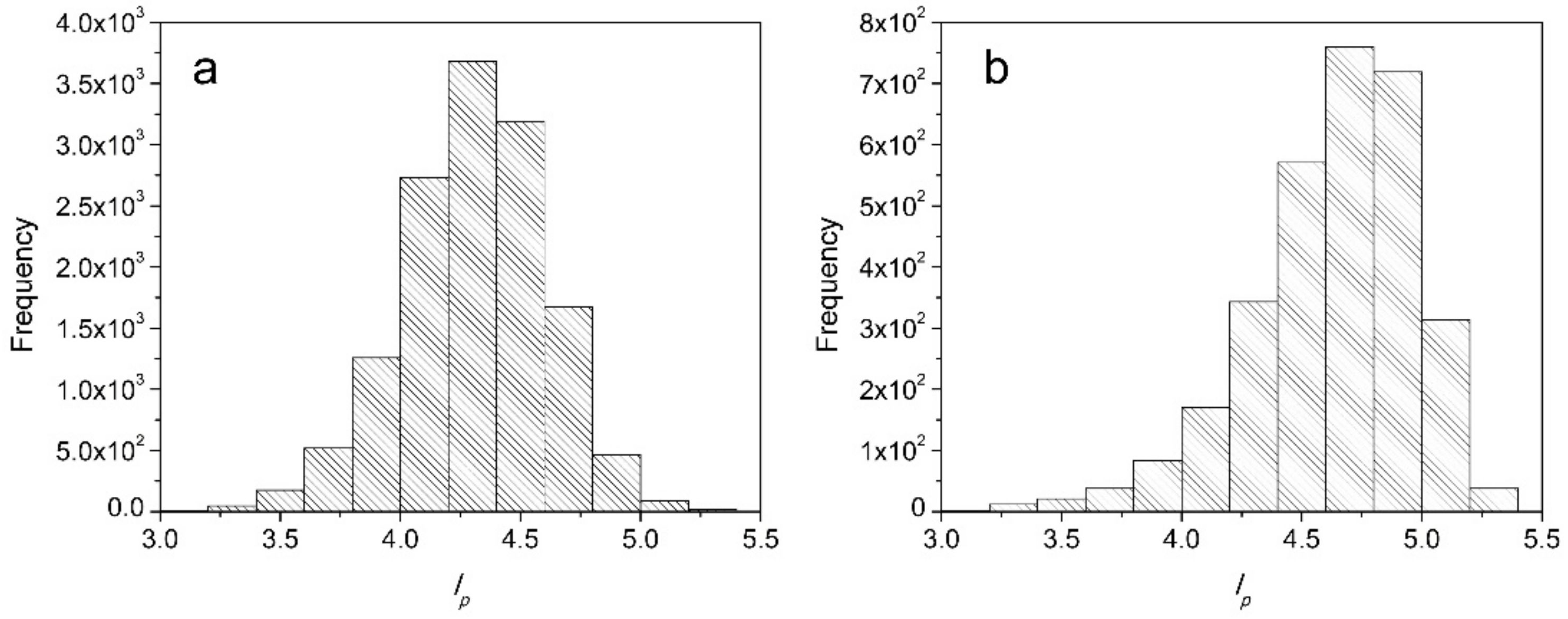The partition ratio between slag and steel quantifies the ability of phosphorous holding onto the slag, given by,$L_p=\frac{{\left(\%\mathrm{P}\right)}_{\mathrm{slag}}}{{\left[\%\mathrm{P}\right]}_{\mathrm{steel}}}$, which indicates the extent of phosphorous removal in the finished steel. Therefore, the extent of dephosphorization can be measured by $L_p$.

Over the years, industries have tried to develop analytical tools to control phosphorous to maintain the quality of products, and many thermodynamics-based mathematical models were developed. In 1974, Balajiva and Vajragupta studied the influences of different chemical compositions of slag on phosphorous removal [5]. The temperature of BOF was kept constant while %CaO, %FeO, and %P2O5 were considered as the controlling factors. Their results showed that an increase in CaO and FeO contents increased the extent of dephosphorization. Suito and Inoue discovered that the phosphorous content in slag is reduced when MnO is added to the slag [6]. Later in 2006, Suito and Inoue conducted experiments to study the behavior of phosphorous transfer from CaO-Fe_tO-P₂O₅(-SiO₂) slags to CaO particles. Based on the results, they developed an equation for the phosphorous partition at the metal-slag interface, given by $\log \left\{\frac{\left(\%P\right)}{\left[\%P\right]}\right\}=0.072\{\left(\%CaO\right)+0.3\left(\%MgO\right)\}+2.5\log \left(\%F{e}_{total}\right)+\frac{11570}{T}-10.52$, where T represents the equilibrium temperature [7]. Assis and Tayeb used 100% direct reduced iron (DRI) in an electric arc furnace (EAF) to investigate the phosphorous equilibrium in different slags [8]. The study has shown that the presence of alumina in slag significantly reduces the phosphorous partition coefficients due to the inactivity of iron oxide. In addition, an equation was developed by Tayeb et al. to describe the relation between phosphorous partition coefficients, slag temperature, and composition, given by, $\log \left(\frac{L_p}{T·F{e}^{2.5}}\right)=0.073\left[\left(\%CaO\right)+0.148\left(\%MgO\right)+0.96\left(\%P_2{O}_5\right)+0.144\left(\%Si{O}_2\right)+0.22\left(\%A{l}_2{O}_3\right)\right]+\frac{11570}{T}-0.46\pm 0.1$. Although simulation of the dynamic reactions is important and effective in many cases of end-point predictions, there are still many uncertainties in the BOF process that are not being captured in even state-of-the-art thermodynamic models owing to the overwhelming numbers of chemical reactions taking place in the process. Therefore, data-driven models are more likely to capture the true non-linear, complex, and stochastic nature of the relationships that exist among the relevant variables in a BOF process.

There are many advantages of using data-driven models over thermodynamic models, and the former one unites and simplifies many complex interactions between factors. A data-driven model learns from large data and evaluates the affecting factors while using none or limited domain knowledge. This factor becomes increasingly handy when the underlying reactions operate at conditions far away from equilibrium. In addition, validation of results is also crucial in building a reliable model used for prediction, and a machine learning (ML) model is a great choice for the situation. ML includes all algorithms that allow the computer to learn from often large data sets and then makes intellectual decisions based on the feedback. The algorithms are built upon the data themselves as it updates and learns from the training data. Recently, multiple linear regression (MLR) model was used to analyze dephosphorization data from the BOF of two steelmakers with different slag basicity and temperatures [9]. Results showed that by reducing the tapping temperature, the phosphorous distribution can be better controlled during steel making. Similarly, Drain et al. developed partition relations between minor slag constituents and dephosphorization of steel and validated those by fitting against a large industrial data set [3]. Their investigation highlighted several important factors; for example, Al₂O₃ was found to have a positive relation with a phosphorous partition at high oxygen potentials and vice versa. Bae et al. explored a range of ML models such as artificial neural network (ANN) and support vector regression (SVR) for the end-point prediction of phosphorous content using a three-year span production data [10]. The 10-fold validation results showed that ANN and SVR perform much better in providing accurate predictions than other algorithms such as extreme gradient boosting (XGBoost) and K-nearest neighbor (KNN). Wang et al. discussed about a multi-level recursive regression model to predict end-point phosphorus [11]. He and Zhang employed principal component analysis combined with a back-propagation neural network on data obtained from a BOF process [12]. Further, Gao et al. introduced an ensemble algorithm combining k-nearest neighbor-based weighted twin support vector regression and Lévy flight whale optimization algorithm [13]. Duo and Zhang implemented a novel multiclass classifier decision tree twin support vector machine based on kernel clustering algorithm [14]. More recently, Phull et al. studied a decision tree-based twin support vector machine to assess the performance of a dephosphorization process using end-point phosphorus content in two BOF steelmaking plants [15]. Indeed, these works imply significant and successful applications of machine learning models for the end-point predictions in BOF. However, either most of these models project and explore dephosphorization as a regression problem [10,11], or not many machine learning models are applied specifically to the dephosphorization process, but rather used to study other measurable components of a BOF process [13,14]. As a result, a detailed investigation is required to further explore the potential of machine learning classifiers (rather than regressors), e.g., support vector machines (SVMs) or other variants of SVM to study the non-linear complex relationships among variables in a BOF process, specifically for dephosphorization.

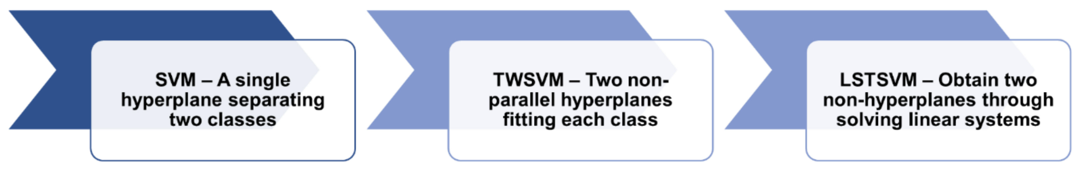
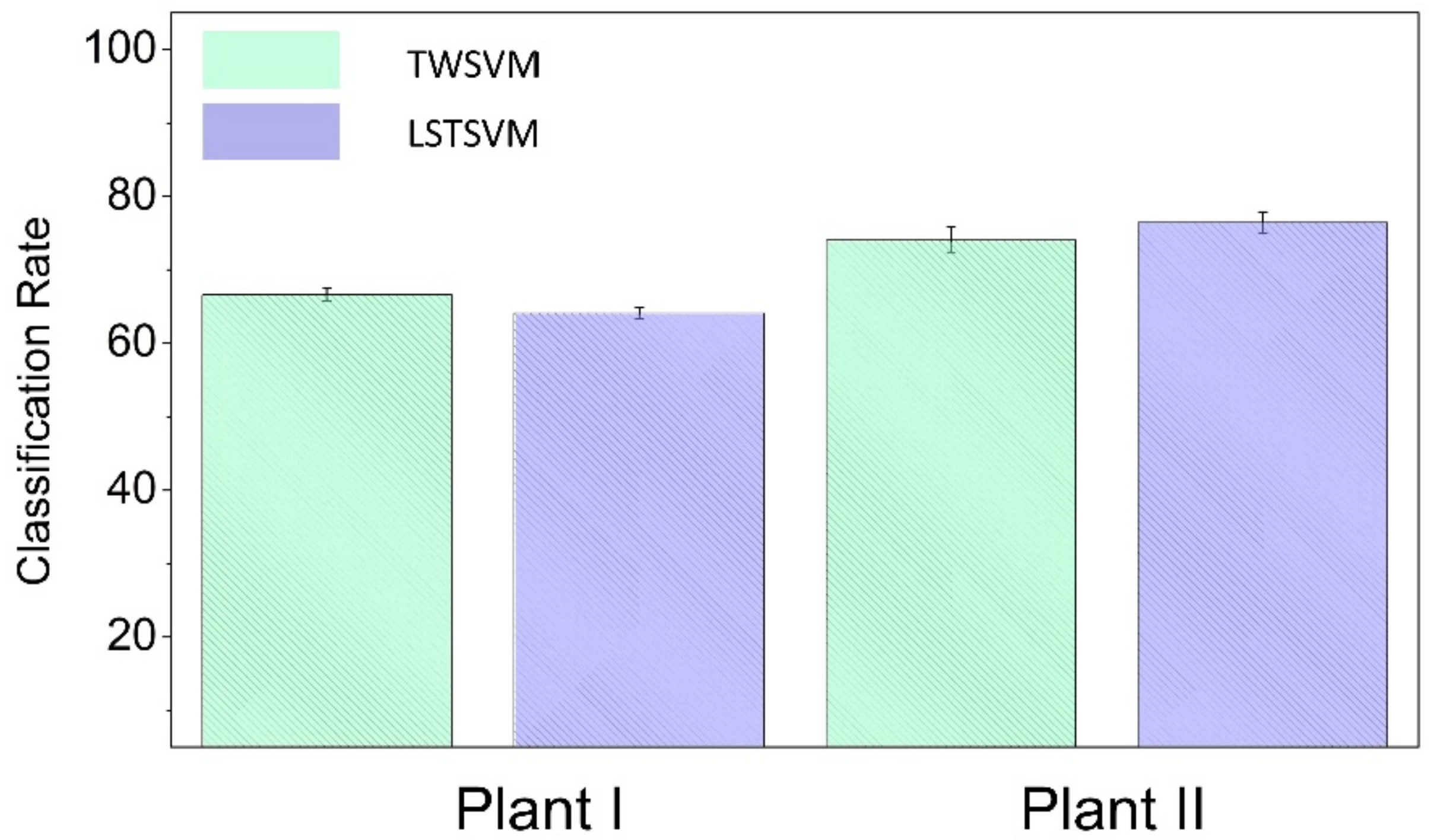
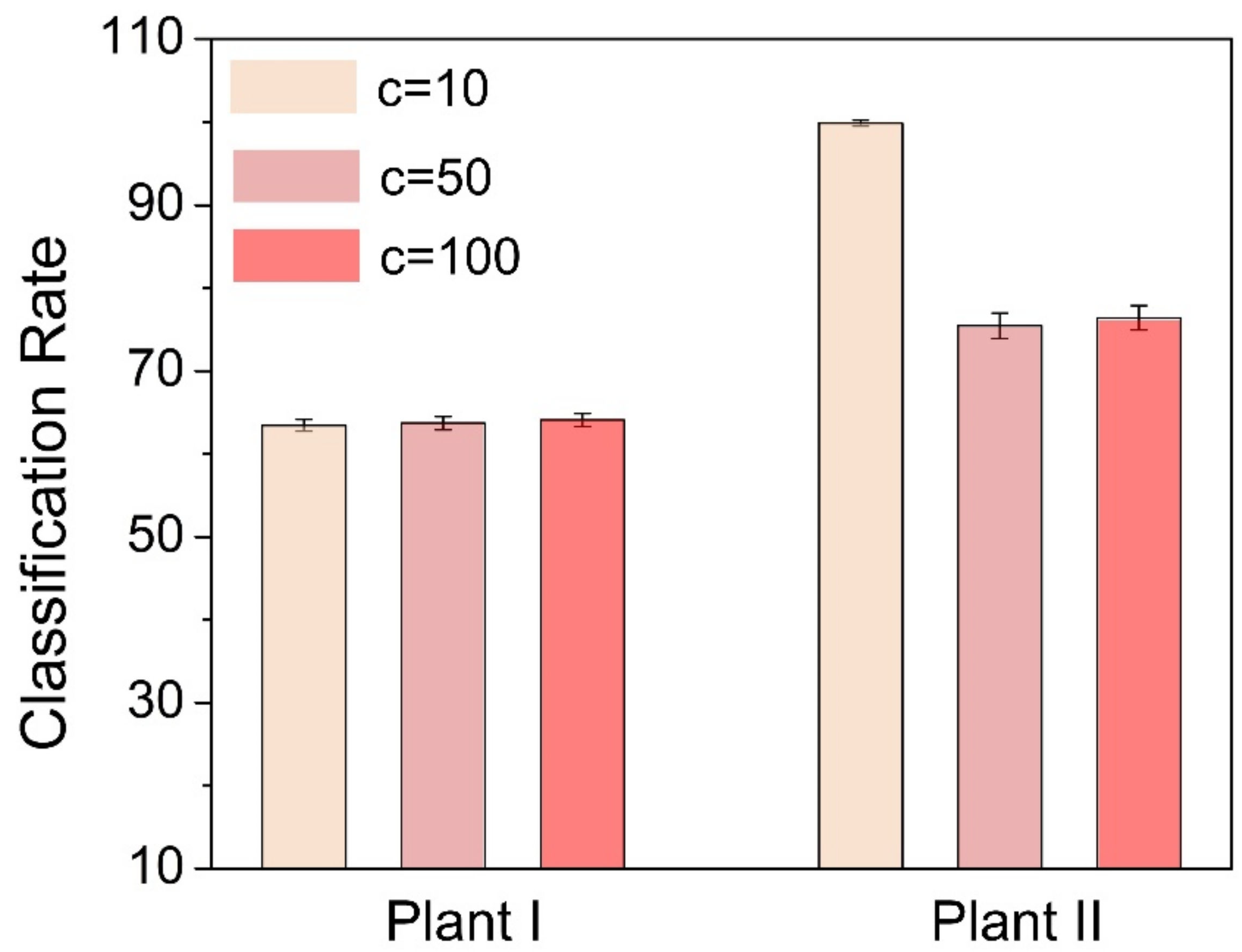
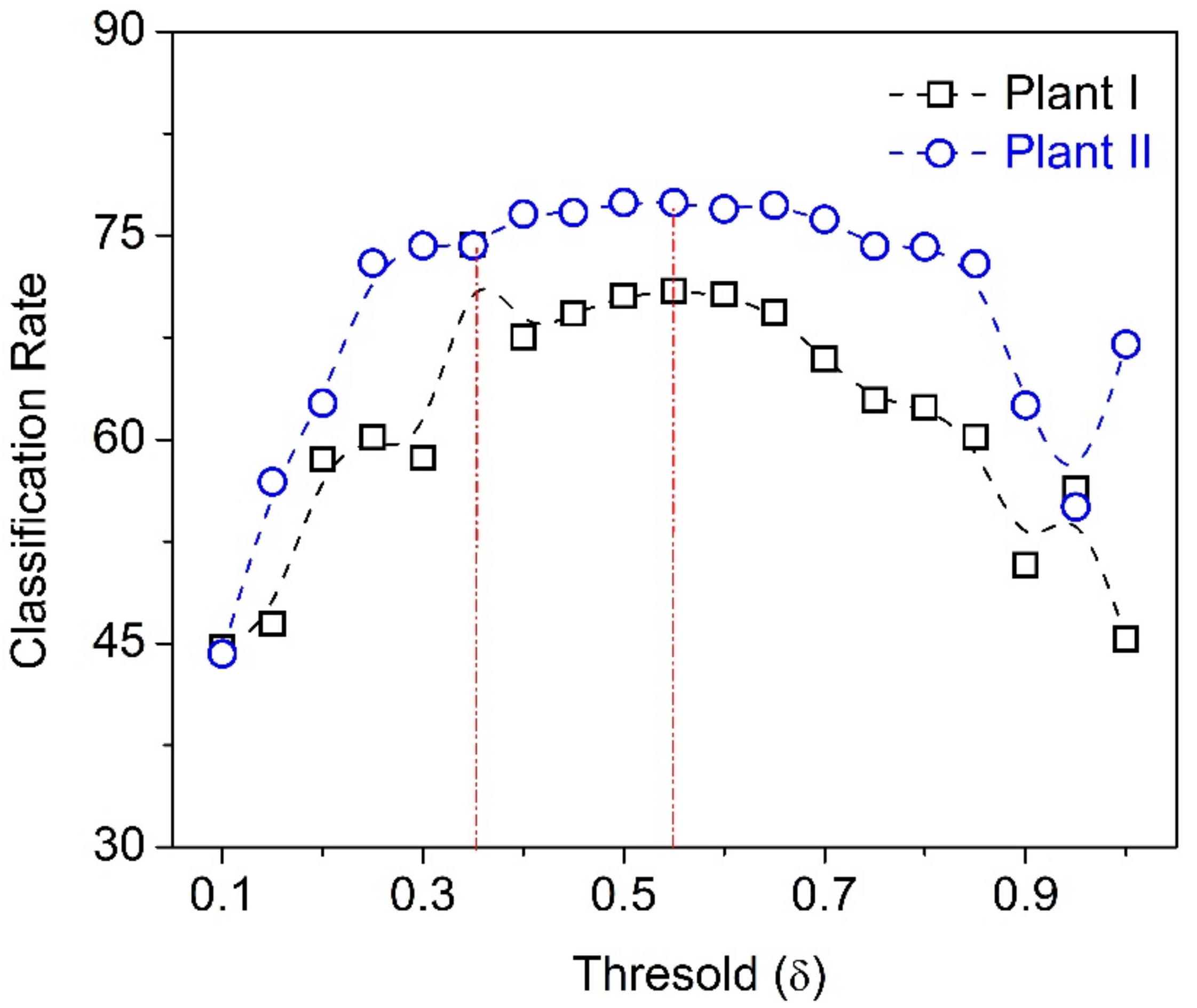
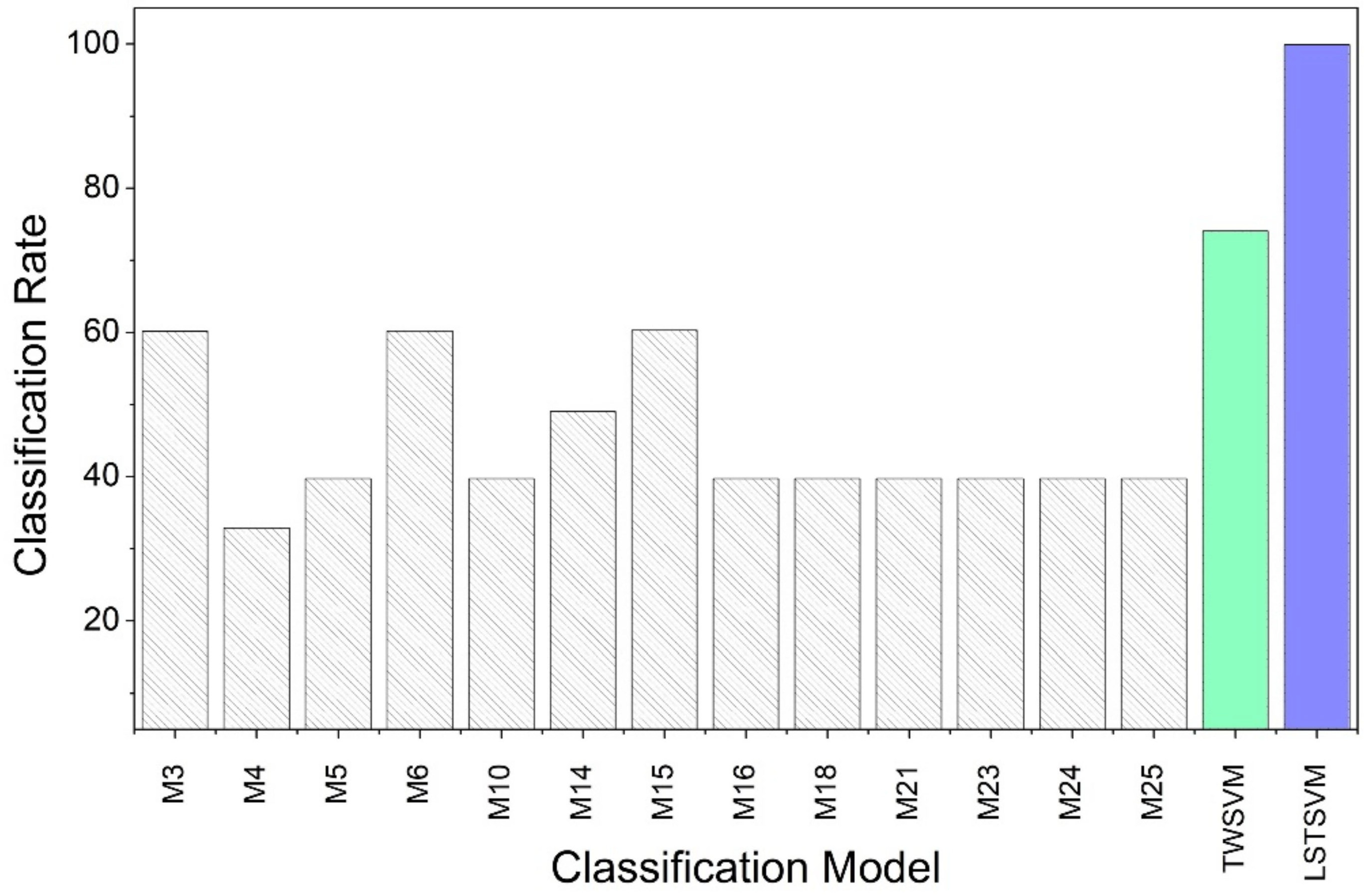
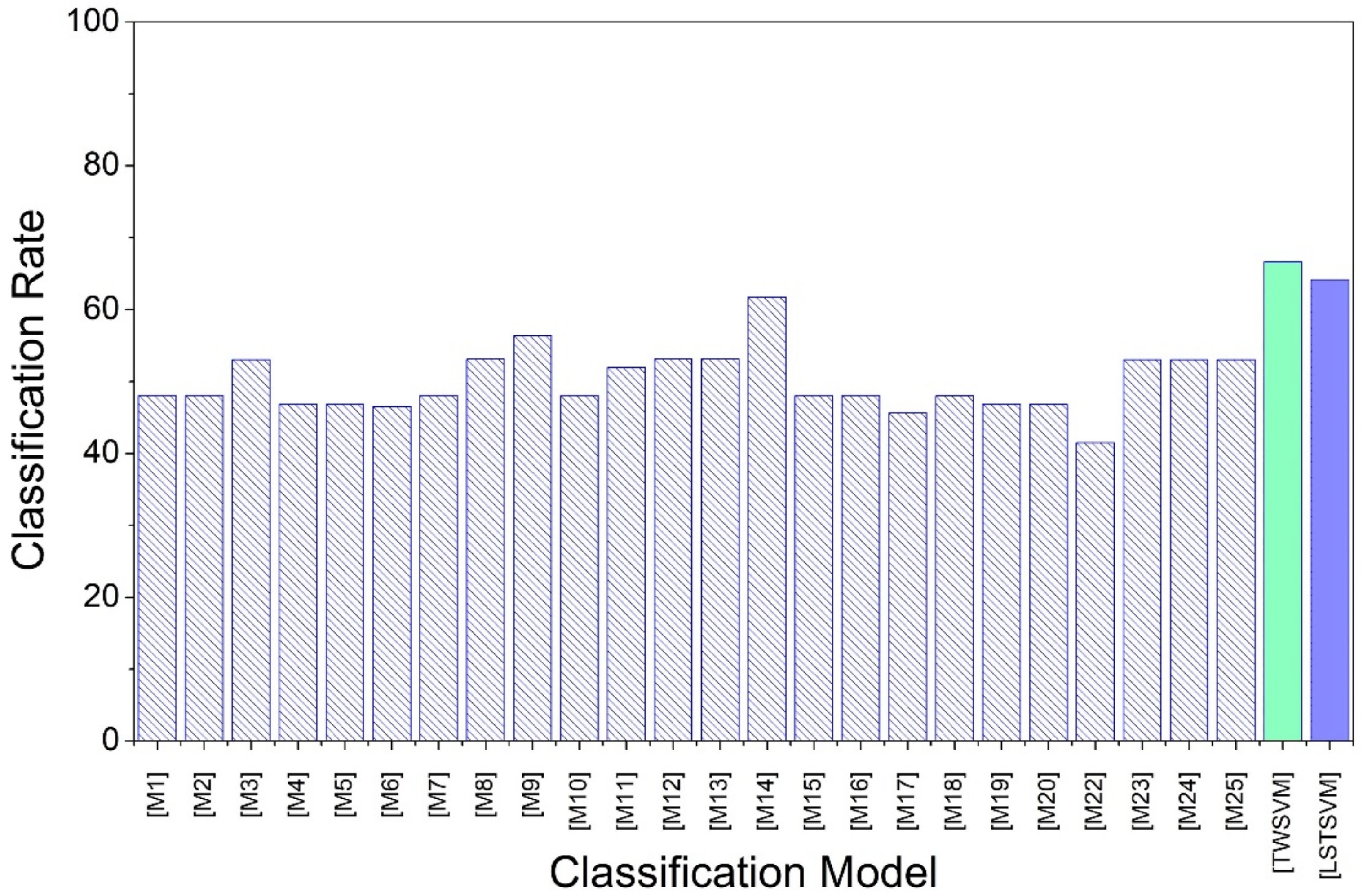
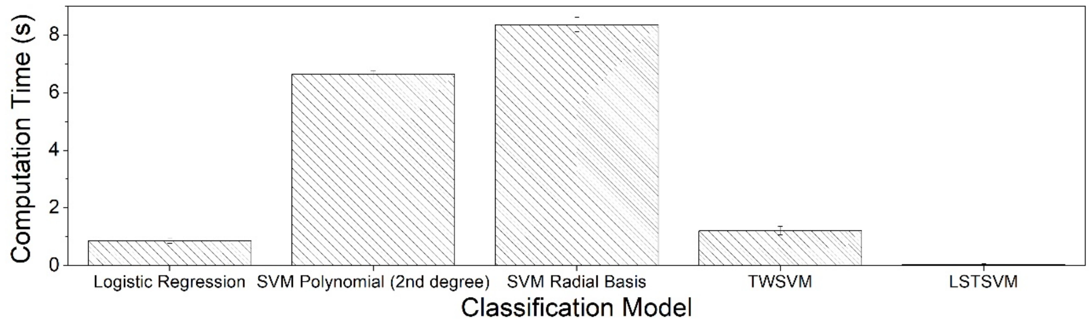
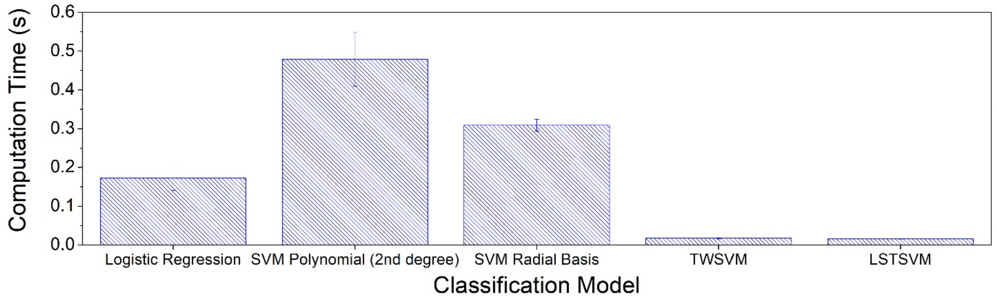
In this article, following the work of Phull et al., ML models are developed using twin support vector machine (TWSVM) and least square twin support vector machine (LSTSVM) for the end-point phosphorous prediction [15]. These models are applied to BOF plant data of two steelmakers in North America. Phosphorous partition is quantified, and the measure is used to classify steel samples based on the chemical composition of slag. The partition values are labeled as Classes 1 and 2 by implementing the K-means clustering algorithm [16,17]. The degree of phosphorous removal is represented through the partition labels. The goal is to implement ML algorithms to predict the partition labeling based on the chemical composition of slag as well as the tapping temperature. TWSVM and LSTSVM are the two ML methods incorporated in the training and testing process. In general, the SVM algorithm determines the best hyperplane as the decision boundary, separating the data into classes. Unlike SVM, TWSVM determines two non-parallel hyperplanes, each fitting one class of data [18,19]. In addition, the computation cost is much less than that of SVM because TWSVM solves a pair of much simplified quadratic programming problems (QPPs). Therefore, for a complex situation such as the phosphorous end-point prediction, TWSVM is preferred over general SVM. LSTSVM is a more appropriate algorithm than TWSVM for data sets with unbalanced classes, as it chooses a different parameter for each class [20,21]. LSTSVM and TWSVM are also preferred over regular SVM when it comes to the large scale and high complexity of QPPs. Consequently, using the mentioned classification algorithms, gradation of the extent of phosphorus removal can be obtained, which can be used to classify a final batch of BOF output to have superior or inferior quality of steel.

2. Theory and Methodology

The purpose of this work is to estimate the extent of phosphorus partition in BOF depending on the chemical composition of slag. Herein, the extent of phosphorous partition (denoted as $l_p$) is quantified as follows:

$$l_p= \ln \left(\frac{\mathrm{Percent}\mathrm{Weight}\mathrm{of}\mathrm{P}\mathrm{in}\mathrm{Slag}}{\mathrm{Percent}\mathrm{Weight}\mathrm{of}\mathrm{P}\mathrm{in}\mathrm{Steel}}\right)=\ln L_p$$

(1)

A higher value of $l_p$ indicates a lower content of phosphorous in steel, which indicates a higher efficiency of the dephosphorization process. TWSVM and LSTSVM with different optimization functions were applied in the characterization of $l_p$ values for the highest accuracy and to optimize the dephosphorization process. $l_p$ values were initially grouped into two classes using the K-means clustering technique. According to the definition of $l_p$, the class with a higher average $l_p$ value is expected to have undergone a greater extent of P removal and vice versa. Therefore, TWSVM and LSTSVM were implemented to classify $l_p$ labels based on the chemical composition of slag and tapping temperatures. All the calculations were performed using the R software v 4.0.4 [22].

2.1. Descriptive Statistics of the Data

Data were collected from two plants (plants I and II) with different average tapping temperatures. The tapping temperatures for plant I was between 1620 and 1650 °C, whereas for plant II this range was slightly higher (between 1660 and 1700 °C). For plant I, 13,853 observations were considered, and each observation had 9 different chemical feature measurements. In plant II, 3084 sets of observations were collected with 7 different chemical features of the slag. The general distribution of the data is displayed in

Table 1. General statistics of the chemical composition of slag in plant I.

Variables	Mean	Standard Deviation	Minimum	Maximum
Temperature °C	1648.82	19.14	1500.00	1749.00
CaO	42.43	3.62	20.00	55.90
MgO	9.23	1.37	3.75	16.46
SiO2	12.89	1.74	5.40	23.30
Fetotal	18.22	3.53	7.70	36.00
MnO	4.80	0.70	2.28	11.98
Al2O3	1.80	0.48	0.59	7.79
TiO2	1.13	0.28	0.17	2.21
V2O5	2.13	0.49	0.25	3.95

and

Table 2. General statistics of the chemical composition of slag in plant II.

Variables	Mean	Standard Deviation	Minimum	Maximum
Temperature °C	1679.10	27.11	1579.00	1777.00
CaO	53.45	2.30	42.33	64.06
MgO	0.99	0.34	0.30	3.18
SiO2	13.52	1.44	8.16	18.74
Fetotal	19.34	2.06	13.71	29.72
MnO	0.62	0.18	0.24	2.50
Al2O3	0.94	0.25	0.46	4.09

below.

Figure 1 represents histograms displaying the data distribution of the two plants based on $l_p$ values after the removal of outliers. These histograms show that $l_p$ values for plant I are distributed symmetrically that for plant II is skewed. This observation could be due to a relatively higher proportion of heats involved in a greater extent of dephosphorization in plant II than in plant I.

2.2. Theory and Modeling

Our implementation has two components: (i) labeling of the $l_p$ values using K-means clustering, and (ii) applying TWSVM and LSTSVM to modify the classification. The purpose is to evaluate the performances of the two methods in classifying the extent of P removal based on the chemical composition of slag. In traditional SVM classification, two classes of data are separated by a hyperplane, which maximizes the distance between data points and the hyperplane. The hyperplane is determined by solving complex QPPs, which is time consuming for a medium or large data set. TWSVM, on the other hand, uses two non-parallel hyperplanes that fit each of the data classes [18,19]. A set of simpler QPPs is solved to determine the hyperplanes. This method is more efficient when compared to regular SVM because the information from one class provides constraints to the other class, which reduces the computation complexity of the algorithm by four times [20,21].

Different from TWSVM, LSTSVM is an improved classification ML algorithm with even faster computational capabilities. LSTSVM solves two linear systems of equations (as opposed to the quadratic ones) while minimizing computational costs. LSTSVM works along a similar line as that of TWSVM in solving two non-parallel planes to fit each class but is more time-efficient for complex data sets. LSTSVM allows for different penalty parameters for different classes, thereby enhancing the speed of the algorithm [17]. A diagrammatic representation of the three related models (SVM, TWSVM and LSTSVM) are presented in Figure 2.

2.2.1. K-Means Clustering

Data were separated into two classes labeled 1 and 2 using the K-means clustering method based on the $l_p$ values [16,17].

2.2.2. Twin Support Vector Machines

After the data sets are separated into two classes based on their corresponding $l_p$ values, the TWSVM algorithm, is applied by fitting two non-parallel hyperplanes into each cluster of data. The two clusters can be represented by two matrices $X_{\mathbf{1}}\in R^{m\times k} \mathrm{and}$ $X_{\mathbf{2}}\in R^{n\times k}$, where $m$ and $n$ are the number of data in each cluster, and $k$ is the number of variables in each set of data. The non-parallel hyperplanes corresponding to each matrix are listed below:

$$x^T{\mathit{w}}_{\mathbf{1}}+b_1=0 \mathrm{and} x^T{\mathit{w}}_{\mathbf{2}}+b_2=0$$

where ${\mathit{w}}_{\mathbf{1}}$ and ${\mathit{w}}_{\mathbf{2}}$ are normal vectors to the hyperplanes, and $b_1$ and $b_2$ are the corresponding bias terms [12]. The hyperplanes can be computed by solving the following objective functions:

$$\begin{gathered} \min \left({\mathit{w}}_{\mathbf{1}},b_1,\mathit{\xi }\right) \frac{1}{2}{\left|\left|X_{\mathbf{1}}{\mathit{w}}_{\mathbf{1}}+{\mathit{e}}_{\mathbf{1}}{b}_1\right|\right|}^2+c_1{\mathit{e}}_{\mathbf{2}}{}^{\mathit{T}}\mathit{\xi } \\ \mathrm{subjected}\mathrm{to} - \left(X_{\mathbf{2}}{\mathit{w}}_{\mathbf{1}}+{\mathit{e}}_{\mathbf{2}}{b}_1\right)+\mathit{\xi } \ge {\mathit{e}}_{\mathbf{2}}, \mathit{\xi }\ge 0 \end{gathered}$$

and

$$\begin{gathered} \min \left({\mathit{w}}_{\mathbf{2}},b_2,\mathit{\xi }\right) \frac{1}{2}{\left|\left|X_{\mathbf{2}}{\mathit{w}}_{\mathbf{2}}+{\mathit{e}}_{\mathbf{2}}{b}_2\right|\right|}^2+c_2{\mathit{e}}_{\mathbf{1}}{}^{\mathit{T}}\mathit{\xi } \\ \mathrm{subjected}\mathrm{to}\left(X_{\mathbf{1}}{\mathit{w}}_{\mathbf{2}}+{\mathit{e}}_{\mathbf{1}}{b}_2\right)+\mathit{\eta } \ge {\mathit{e}}_{\mathbf{1}}, \mathit{\eta }\ge 0 \end{gathered}$$

where $\mathit{\eta }$ and $\mathit{\xi }$ are slack variables, and $c_1$ and $c_2$ are penalty parameters. Further, ${\mathit{e}}_{\mathbf{1}}$ and ${\mathit{e}}_{\mathbf{2}}$ are two vectors of suitable dimensions with values of all 1s. To find a solution, Lagrange multipliers are introduced to simplify the problem [18]. Testing data samples will be assigned to each group according to the perpendicular distance from each data to the hyperplane, and the decision function is expressed as:

$$\mathrm{Class} i=\min \left|{\mathbf{x}}^{\mathbf{T}}{\mathit{w}}_{\mathit{i}}+b_i\right| \mathrm{for} i=1, 2.$$

2.2.3. Least Squares Twin Support Vector Machines

LSTSVM generates two non-parallel hyperplanes by solving two linear systems of equations, and the solutions are obtained through the following optimization problems [20,21]:

$$\begin{gathered} \min \left({\mathit{w}}_{\mathbf{1}},b_1,\mathit{\xi }\right) \frac{1}{2}{\left|\left|{\mathbf{X}}_{\mathbf{1}}{\mathit{w}}_{\mathbf{1}}+\mathit{e}{b}_1\right|\right|}^2+\frac{c_1}{2}{\mathit{\xi }}^{\mathit{T}}\mathit{\xi } \\ \mathrm{subjected}\mathrm{to} -\left({\mathbf{X}}_{\mathbf{2}}{\mathit{w}}_{\mathbf{1}}+\mathit{e}{b}_1\right)+\mathit{\xi }=\mathit{e} \end{gathered}$$

and

$$\begin{gathered} \min \left({\mathit{w}}_{\mathbf{2}},b_2,\mathit{\eta }\right) \frac{1}{2}{\left|\left|{\mathbf{X}}_{\mathbf{2}}{\mathit{w}}_{\mathbf{2}}+\mathit{e}{b}_2\right|\right|}^2+\frac{c_2}{2}{\mathit{\eta }}^{\mathit{T}}\mathit{\eta } \\ \mathrm{subjected}\mathrm{to} \left({\mathbf{X}}_{\mathbf{1}}{\mathit{w}}_{\mathbf{2}}+\mathit{e}{b}_2\right)+\mathit{\eta }=\mathit{e}. \end{gathered}$$

The assignment of data sample will take place as follows:

$$\mathrm{Class} i=\arg \min \left(j = 1,2\right)\frac{\left|{\mathit{w}}_{\mathit{j}}^{\mathit{T}}\mathit{x}+b_j\right|}{||{\mathit{w}}_{\mathit{j}}||}$$

2.3. Model Validation and Performance Measures

The models’ tuning parameters were adjusted by comparing the accuracy of the test results against the true clustering results. To maintain a margin large enough when the distribution overlaps, a penalty parameter $c$ was introduced to regularize the cost function. A large penalty parameter leads to a smaller margin and larger training accuracy, while a small penalty parameter results in a smaller training accuracy. A larger margin prevents overfitting, and thus, the parameters were tuned based on the margin and accuracy trade-off.

Both models randomly selected 80% of the total data from each data set (i.e., plant I and plant II) for training and the other 20% for testing. The accuracy of the classification methods was calculated through the classification table and is given by [16,17]:

$$\mathrm{Classification}\mathrm{Rate}=\frac{\mathrm{True}\mathrm{Positives}+\mathrm{True}\mathrm{Nagatives}}{\mathrm{Total}\mathrm{Sample}\mathrm{Size}}$$

(2)

Classification rates were measured for 100 random dynamic train-test splits to demonstrate the consistency of the accuracy of the model by normalizing over random noises that may occur. The average over these 100 runs is presented as the accuracy of a model. Along with the average, standard deviation, minimum and maximum over all 100 runs were estimated to further ascertain the accuracy, robustness, and consistency of the binary classification techniques.

• To demonstrate the model performances, we compared results from TWSVM and LSTSVM against the logistic regression model. Logistic regression is a statistical method of regressing where the probability (P) of the response variable belonging to a group is estimated based on feature variables by using likelihood-based estimation [23]. If Y is the response variable ($l_p$ in our analysis) and Y can belong to either group ‘0’ or ‘1’ (Class 1 or Class 2 in our analysis), then

$$\mathrm{P}\left(\mathrm{Y}=1\right) ={\left[1+e^{-\left({\beta }_0+{\beta }_1{x}_1+{\beta }_2{x}_2+\cdots +{\beta }_p{x}_p\right)}\right]}^{-1}$$

(3)

where $p$ represents the number of features, and ${\beta }_0,{\beta }_1\dots , {\beta }_p$ are the regression coefficients [24]. This regression technique can be converted to a classification method by choosing an appropriate threshold value $\delta \in \left[0,1\right]$. If $\widehat{\mathrm{P}\left(\mathrm{Y}=1\right)}>\delta$ then Y takes the value ‘1’, else Y takes ‘0’, where $\widehat{\mathrm{P}\left(\mathrm{Y}=1\right)}$ is the estimated value of $\mathrm{P}\left(\mathrm{Y}=1\right)$ using (3). After fitting the logistic regression model on 80% training data from plants I and II, confusion matrices were constructed on the 20% test data in the same way mentioned in (2). A grid search was performed over $\delta$ in the interval [0,1] with an increment of 0.05, and the one that returned the highest accuracy (classification rate) was chosen. To average out noises and establish consistency, the process was repeated 100 times for each threshold value, and their mean accuracies were observed.

• Besides the ML algorithms used in recent years, there have been many regression models (based on thermodynamic or empirical concepts) that predicts the $l_p$ values from other chemical compositions of slag. In 2019, Barui et al. selected 25 existing regression models and tested their performances against their own data-driven linear regression model using RMSE and R² values [25]. In this article, we compared our classification models (TWSVM and LSTSVM) against those 25 regression models that were applied to plant I and plant II data for classification. Interested readers may refer to Barui et al. for the detailed list of these 25 predictive model equations. We considered the same numbering system of the 25 equations (namely, (M1)–(M25)) as adopted by Barui et al. Not all equations could be used for comparisons for both plants’ data due to the lack of complete information. Of those 25 models, 13 were available for comparisons for the plant I data, while 24 were used for the plant II data. For each heat, $l_p$ values were predicted (${\widehat{l}}_p$) based on the chemical composition of slag and tapping temperature using the equations among (M1)–(M25), whichever were applicable. On the other hand, by using K-means clustering, we obtained the two clusters (Classes 1 and 2) and their respective $l_p$ averages, say ${\overline{l}}_{p1}$ and ${\overline{l}}_{p2}$. A particular heat was classified to $\mathrm{Class} i$ by the following assignment rule:

$$\mathrm{Class} i=\arg \min \left(j=1, 2\right)\left\{\mathrm{dist}\left({\widehat{l}}_p,{\overline{l}}_{pj}\right)\right\}$$

Once the assignments were over for all heats, the accuracies of the predictive model equations were measured by the classification rate as mentioned in (2).

3. Results

3.1. Labeling of $l_p$ and Statistics of the Classes

The frequency, mean, standard deviation, minimum, and maximum for each cluster of $l_p$ values, namely, Classes 1 and 2, after the application of the K-means clustering method, are presented in

Table 3. Descriptive statistics of $l_p$ values for Classes 1 and 2 for plant I.

	Frequency (%)	Mean	Standard Deviation	Minimum	Maximum
Class 1 (L)	6097 (44.01%)	4.04	0.19	2.50	4.27
Class 2 (H)	7756 (55.99%)	4.52	0.18	4.28	7.06

and

Table 4. Descriptive statistics of $l_p$ values for Classes 1 and 2 for plant II.

	Frequency (%)	Mean	Standard Deviation	Minimum	Maximum
Class 1 (L)	1035 (33.59%)	4.24	0.26	2.76	4.53
Class 2 (H)	2046 (66.41%)	4.82	0.17	4.53	5.64

for both the plants. For plant I, data from 6097 heats are found to belong to Class 1 and 7756 to Class 2, whereas for plant II there are 1035 data points belonging to Class 1 and 2046 assigned to Class 2. In addition, the standard deviations are of similar magnitudes. For both plants, Class 1 represents the class with ‘Low’ degree of phosphorus removal, whereas Class 2 represents the one with a ‘High’ degree of dephosphorization. The bifurcation is evident on observing the mean, minimum and maximum $l_p$ values. The range of the $l_p$ values spans between 2.50 and 7.06, implying a high level of dispersion across heats.

3.2. Optimization and Performance

Lagrange multipliers were used to solve the hyperplane equations, which were obtained from the Wolfe dual optimization functions [18]. Three methods, namely, a general-purpose optimization based on the Nelder–Mead method, spectral projected gradient (SPG), and quasi-Newton algorithms included in the wrapper function, were used for optimization [26,27,28]. For the Nelder–Mead method, a simplex is used to search for the optimal solution. The simplex changes its shape and traverses in space to move toward the minimum. Targeting convex constrained problems, SPG is a hybrid method of spectral nonmonotone concepts and classical projected gradient techniques. Quasi-Newton optimization is another gradient-based method that searches for a function’s maxima and minima. This method requires a gradient of the function to build on the second-order information, which is the Hessian matrix. The quasi-Newton method works best for medium-sized data but is not efficient for large data sets. From the results, the Nelder–Mead method provided the most optimal performance at the lowest computational cost.

The classification rates of the TWSVM and LSTSVM models are provided in

Table 5. Model performances in terms of classification rate for plant I and plant II data.

TWSVM
Plant	$c$	Mean	Standard Deviation	Minimum	Maximum
I	-	0.6662	0.0082	0.6435	0.6835
II	-	0.7404	0.0179	0.6932	0.7744
LSTSVM
Plant	$c$	Mean	Standard Deviation	Minimum	Maximum
I	10	0.6346	0.0071	0.6146	0.6532
I	50	0.6372	0.0080	0.6193	0.6561
I	100	0.6410	0.0078	0.6207	0.6619
II	10	0.9990	0.0036	0.9789	1.0000
II	50	0.7546	0.0153	0.7143	0.8036
II	100	0.7643	0.0147	0.7305	0.8019

. From Table 5, it is observed that the accuracy percentages reach almost 100% while classifying $l_p$ by applying LSTSVM on plant II data when the penalty parameter $c=10$. On the contrary, the same penalty parameter value resulted in a classification rate of approximately 63% for the plant I data. The classification rate across different penalty parameter values ($c=10, 50$ and $100$) by LSTSVM for the plant I data showed a similar trend (63.46–64.10%). However, the classification rate by LSTSVM for plant II data is the lowest (75.46%) for $c=50$ and highest (99.90%) for $c=10$. On average, TWSVM performs marginally better (accuracy of 66.62%) as opposed to LSTSVM (accuracy of 64.10%) for plant I data, whereas LSTSVM (accuracy of 99.90%) outperforms TWSVM (accuracy of 74.04%) when applied to plant II data. Graphical representations of the classification rate are shown in Figure 3 and Figure 4 with the aid of bar plots. The standard deviations for both classification models and various penalty parameters values are low in comparison to the respective means signifying less variability across 100 runs. This suggests the insensitivity of accuracy measures with respect to the split in training and test data.

The performance of the logistic regression-based classifications is given in

Table 6. Performance of the logistic regression-based classification for plants I and II.

Logistic Regression Classifier
Plant	$\mathbf{Threshold} \left(\mathit{\delta }\right)$	Mean	Standard Deviation	Minimum	Maximum
I	0.05	0.4469	0.0089	0.4273	0.4630
I	0.10	0.4643	0.0089	0.4370	0.4857
I	0.50	0.7090	0.0071	0.6011	0.7279
I	0.80	0.6017	0.0092	0.5778	0.6254
II	0.05	0.4422	0.0226	0.3890	0.5089
II	0.10	0.5490	0.0216	0.4830	0.5948
II	0.50	0.7739	0.1450	0.3710	0.8023
II	0.80	0.7290	0.0167	0.6807	0.7715

. We computed the mean, standard deviation, minimum and maximum of the classification rates over 100 Monte Carlo runs of random 80–20% train-test split for every $\delta =0.05, 0.10,\dots , 0.95$. For brevity, we just presented the values for $\delta =0.05, 0.10, 0.50, 0.80$ in Table 6. On the other hand, Figure 5 shows the mean classification rates of the logistic regression model for both plants I and II for every $\delta =0.05, 0.10,\dots , 0.95$. For $\delta =0.30$ and $\delta =0.50$, the highest accuracies in terms of the classification rates were observed for plants I and II, respectively (see Figure 5). LSTSVM provided with better accuracy (99.90%) as compared to the logistic regression model (accuracy of 77.39%) for plant II data, whereas the latter has a greater classification rate (accuracy of 74.31%) than both TWSVM (accuracy of 66.62%) and LSTSVM (accuracy of 64.10%) for the plant I data.

As mentioned in Section 2.3, the performances based on the classification rates of our proposed models were compared against the 25 regression equations discussed by Barui et al. These 25 equations, along with their references, are also provided in Table S1. in the supplementary materials of this paper. Figure 6 and Figure 7 reveal that the highest accuracies were attained by the equation (M15) (with an accuracy of 60.30%) for plant I and by the equation (M14) (with an accuracy of 61.70%) for plant II. Nevertheless, the classification rates were lesser than the TWSVM and LSTSVM models for all cases. Some equations (e.g., (M16), (M18), (M21), (M23), (M24) for plant I) were found to have equal classification rates because they all have predicted either too high or too low $l_p$ values than the K-means cluster averages. Hence, all observations were classified to just one cluster for those equations resulting in skewed accuracies. From the results, it can be concluded that these regression models do not perform as well as the proposed TWSVM and LSTSVM algorithms.

The main advantage of applying LSTSVM over other fitted models is in terms of computation or running time. As shown in

Table 7. Average running time (in seconds) of the applied classification models per 100 runs for plant I and plant II data.

Model	Plant I	Plant II
Logistic Regression	0.8577	0.1730
SVM Polynomial (2nd Degree)	6.6370	0.4793
SVM Radial Basis	8.3610	0.3090
TWSVM	1.2130	0.0175
LSTSVM	0.0500	0.0167

, the average running times of logistic regression, SVM with both polynomial and radial basis function (RBF) kernels, TWSVM, and LSTSVM with their best-performing parameters are recorded. For each model, the test is repeated 100 times with randomly selected data, and the total time is noted. Then the total time is divided by 100 to show the time taken for each prediction. The run time of each prediction improves significantly in LSTSVM compared with the other models. As discussed before, the SVM models and their variants are tuned for the best combinations of hyperparameters. It can be clearly seen from Table 7 that LSTSVM is approximately 167 times faster than SVM with RBF kernel for large data set (Plant I) and 18 times for small data set (plant II). LSTSVM shows 1.5–24 times lesser computation times than TWSVM. Figure 8 and Figure 9 represent results from Table 7 graphically.

4. Discussion

4.1. Algorithm Performance

All data points were normalized before applying the algorithms for classification to reduce both consumption of computational resources and aid comparability by bringing all variables down at the same scale. Looking at the classification rates obtained from both algorithms (Figure 4), LSTSVM produced an accuracy of almost 25% greater with $c=10$ for plant II data than TWSVM, while TWSVM outperformed LSTSVM by a marginal 2% for plant I data. Furthermore, on average, after applying both algorithms, the accuracy obtained for plant I data by applying both algorithms is lower than plant II. Similar observations were made by Phull et al. in their work where the same data sets were analyzed by a decision tree-based TWSVM algorithm [15]. This discrepancy in accuracy could have the following plausible explanation: Plant I has a larger data set (almost five times) in comparison to plant II, and the $l_p$ distribution for plant II is more negatively skewed than that of plant I. Data from 13,853 heats and 9 chemical features were observed for plant I, and only 3084 observations and 7 chemical features were considered from plant II for the study. Two additional features, namely V₂O₅ and TiO₂, were considered in the classification models for the plant I data. Although large data sets generally result in smaller bias, however, they may also exhibit higher variability and a noisy pattern, which can diminish the accuracy of the ML algorithms. As shown in Figure 1, the $l_p$ distribution for plant II is more skewed to the left, whereas plant I is almost normally distributed. This condition indicates that the $l_p$ values reside more on the higher range for plant II and are more symmetrically spread out across all observations for plant I. Further, the initial clusters obtained by using the K-means clustering algorithm to the data had a split ratio of 45–55% for plant I and 34–66% division ratio for plant II. The ratio points toward the asymmetry in the data distribution for plant II. Therefore, it is easier to separate the values into two classes for plant II, which could result in a higher classification rate in the algorithm. From our study, it is fair to conclude that LSTSVM outperforms TWSVM when the initial data clusters are disproportionate with respect to the number of observations while performing almost similar to that of TWSVM for proportionately distributed clusters.

The performances of our proposed models (TWSVM and LSTSVM) were compared against the logistic regression-based classifier and 25 well-established data-driven regression equations (adapted for classification) discussed by Barui et al. LSTSVM outperforms all classification models considered for comparison for the plant II data [25]. On the contrary, the logistic regression model performs best for the plant I data. The probable reasons for this discrepancy have been discussed above. All three classification models, namely, TWSVM, LSTSVM, and logistic regression-based classifier, perform better than the 25 predictive models discussed in Barui et al.

Because LSTSVM solves two linear systems of equations while TWSVM solves a pair of QPPs (though much simple in complexity than that of the regular SVM), LSTSVM computes at a considerably faster speed than TWSVM does in the training process. The superiority of LSTSVM over other applied algorithms is evident in Table 7. Therefore, training models with very large data sets (big data) LSTSVM would be extremely time and cost efficient.

This efficiency in computation can be a major advantage in an industrial setting. It is also worth noting that the classification rate for plant II increases with lower cost parameters, and this is because a lower cost results in a larger margin. A larger margin sets a better possible separation between the two classes and thus performs better on validation data.

4.2. Applications to the Steel Industry and Future Work

These ML algorithms can be applied to the steel manufacturing industry to tackle not only dephosphorization but to efficiently maintain end-point control in the BOF process, where the end-point phosphorous parameters could be predicted with a given chemical composition of slag and tapping temperatures. In our current study, the $l_p$ value is separated into two classes, in which Class 1 represents the group with a lower extent of phosphorus partition and Class 2 represents a higher degree of phosphorous removal. The proposed method is a reliable structure that takes in the values of the chemical composition of slag and tapping temperature and computes the cluster its corresponding $l_p$ belongs to, allowing for manufacturing improved finished product. In addition, the computational time of LSTSVM is significantly reduced from that of traditional SVM and TWSVM, as shown in Table 7. The reduced run time poses the advantage of the proposed algorithm, allowing easy use in the industrial setting when they do not have access to high-end computational tools. With more comprehensive data, we can adjust the initial labeling to be more precise by clustering the $l_p$ values into classes. The goal of the dephosphorization process is to produce a grade of steel that falls in the higher class for the process to be efficient. This improvement would lead to a more accurate prediction of the $l_p$ value, and the ML models could predict the final content with careful adjustment of the process parameters. Although TWSVM and LSTSVM show promising results in their classification performance, LSTSVM would be a better fit in a shop floor setting because of its faster speed and easier implementation by computing linear systems of equations, especially when dealing with higher dimensional real-time data.

5. Concluding Remarks

Least squares twin support vector machines, a modified version of the twin support vector machines, which itself is an extension of ordinary support vector machines, is proposed in this paper for the binary classification of the phosphorus ‘partition’ ratio denoted by $l_p$. The classes, denoted by Class 1 and Class 2, represent the respective lower and a higher degree of phosphorus removal in steel in the BOF steelmaking process. An unsupervised ML algorithm of K-means clustering is implemented for the initial labeling of each heat observation based on the $l_p$ values. LSTSVM is a fast and simple alternative to the TWSVM, which solves two systems of linear equations as opposed to solving two systems of quadratic programming problems. Data from two BOF plants (plant I and plant II) were explored for studying the performance of the proposed algorithms. LSTSVM achieved an accuracy of around 64% for plant I data and 99.9% for plant II data. On average, LSTSVM outperformed TWSVM when the data distribution is skewed, as in the case of plant II. It is further observed that increasing the number of features or data points does not necessarily improve the accuracy of the suggested models. To further exemplify the performance of LSTSVM, it was compared against the logistic regression model as well as already existing 25 data-driven predictive models. For the plant II data, LSTSVM delivered the highest classification rate among all these classification models.

The rapidity of the algorithms could be used in actual industrial settings or BOF shops generating real-time data for end-point phosphorus classification. By carefully manipulating the chemical composition of slag and tapping temperature for a particular heat in subsequent batches, a greater degree of phosphorus removal could be achieved within a short span of time by channelizing the structure of the proposed classification algorithm. Other efficient variations of the TWSVM could be studied in the context of dephosphorization as a part of future works.

References

1. Miller, T.W.; Jimenez, J.; Sharan, A.; Goldstein, D.A. Oxygen Steelmaking Processes. In The Making, Shaping and Treating of Steel-Steelmaking and Refining; AISE Steel Foundation: Pittsburgh, PA, USA, 1998; pp. 457–524. [Google Scholar]
2. Pig Iron: Meaning and Impurities|Metals|Industries|Metallurgy, Engineering Notes India. 2020. Available online: https://www.engineeringenotes.com/metallurgy/iron/pig-iron-meaning-and-impurities-metals-industries-metallurgy/20784 (accessed on 26 January 2022).
3. Drain, P.B.; Monaghan, B.J.; Zhang, G.; Longbottom, R.J.; Chapman, M.W.; Chew, S.J. A review of phosphorus partition relations for use in basic oxygen steelmaking. Ironmak. Steelmak. 2017, 44, 721–731. [Google Scholar] [CrossRef] [Green Version]
4. Basu, S.; Lahiri, A.; Seetharaman, S. Phosphorus Partition between Liquid Steel and CaO-SiO2-FeOx-P2O5-MgO Slag Containing 15 to 25 Pct FeO. Metall. Mater. Trans. B 2007, 38, 623–630. [Google Scholar] [CrossRef]
5. Balajiva, K.; Quarrell, A.G.; Vajragupta, P. A laboratory investigation of the phosphorus reaction in the basic steelmaking process. J. Iron. Steel. Inst. 1946, 153, 115. [Google Scholar]
6. Suito, H.; Inoue, R. Phosphorus distribution between MgO-saturated CaO-FetO-SiO2-P2O5-MnO slags and liquid iron. Trans. Iron Steel Inst. Jpn. 1984, 24, 40–46. [Google Scholar] [CrossRef]
7. Suito, H.; Inoue, R. Behavior of Phosphorous Transfer from CaO-FetO-P2O5(-SiO2) Slag to CaO Particles. ISIJ Int. 2006, 46, 180–187. [Google Scholar] [CrossRef] [Green Version]
8. Assis, A.N.; Tayeb, M.A.; Sridhar, S.; Fruehan, R.J. Phosphorus Equilibrium between Liquid Iron and CaO-SiO2-MgO-Al2O3-FeO-P2O5 Slags: EAF Slags, the Effect of Alumina and New Correlation. Metals 2019, 9, 116. [Google Scholar] [CrossRef] [Green Version]
9. Chattopadhyay, K.; Kumar, S. Application of thermodynamic analysis for developing strategies 496 to improve BOF steelmaking process capability. In Proceedings of the AISTech 2013 Iron and 497 Steel Technology Conference, Pittsburgh, PA, USA, 6 May 2013; pp. 809–819. [Google Scholar]
10. Bae, J.; Li, Y.; Ståhl, N.; Mathiason, G.; Kojola, N. Using Machine Learning for Robust Target Prediction in a Basic Oxygen Furnace System. Met. Mater. Trans. A 2020, 51, 1632–1645. [Google Scholar] [CrossRef]
11. Wang, Z.; Xie, F.; Wang, B.; Liu, Q.; Lu, X.; Hu, L.; Cai, F. The Control and Prediction of End-Point Phosphorus Content during BOF Steelmaking Process. Steel Res. Int. 2014, 85, 599–606. [Google Scholar] [CrossRef]
12. He, F.; Zhang, L. Prediction model of end-point phosphorus content in BOF steelmaking process based on PCA and BP neural network. J. Process Control 2018, 66, 51–58. [Google Scholar] [CrossRef]
13. Gao, C.; Shen, M.; Liu, X.; Wang, L.; Chen, M. End-point Prediction of BOF Steelmaking Based on KNNWTSVR and LWOA. Trans. Indian Inst. Met. 2018, 72, 257–270. [Google Scholar] [CrossRef]
14. Dou, Q.; Zhang, L. Decision Tree Twin Support Vector Machine Based on Kernel Clustering for Multi-class Classification. In International Conference on Neural Information Processing; Springer: Cham, Switzerland, 2018; pp. 293–303. [Google Scholar] [CrossRef]
15. Phull, J.; Egas, J.; Barui, S.; Mukherjee, S.; Chattopadhyay, K. An Application of Decision Tree-Based Twin Support Vector Machines to Classify Dephosphorization in BOF Steelmaking. Metals 2019, 10, 25. [Google Scholar] [CrossRef] [Green Version]
16. James, G.; Witten, D.; Hastie, T.; Tibshirani, R. An Introduction to Statistical Learning; Springer: New York, NY, USA, 2013; Volume 112. [Google Scholar]
17. Friedman, J.; Hastie, T.; Tibshirani, R. The Elements of Statistical Learning; Springer Series in Statistics: New York, NY, USA, 2001; Volume 1. [Google Scholar]
18. Khemchandani, R.; Chandra, S. Twin Support Vector Machines for Pattern Classification. IEEE Trans. Pattern Anal. Mach. Intell. 2004, 26, 4. [Google Scholar]
19. Tomar, D.; Agarwal, S. Twin Support Vector Machine: A review from 2007 to 2014. Egypt. Inform. J. 2015, 16, 55–69. [Google Scholar] [CrossRef]
20. Chen, S.; Xu, J. Least Squares Twin Support Vector Machine for Multi-Class Classification. Int. J. Database Theory Appl. 2015, 8, 65–76. [Google Scholar] [CrossRef]
21. Mitra, V.; Wang, C.-J.; Banerjee, S. Text classification: A least square support vector machine approach. Appl. Soft Comput. 2007, 7, 908–914. [Google Scholar] [CrossRef]
22. R-project.org. R: The R Project for Statistical Computing. 2021. Available online: https://www.r-project.org/ (accessed on 26 January 2022).
23. Dreiseitl, S.; Ohno-Machado, L. Logistic regression and artificial neural network classification models: A methodology review. J. Biomed. Inform. 2002, 35, 352–359. [Google Scholar] [CrossRef] [Green Version]
24. Kurt, I.; Ture, M.; Kurum, A. Comparing performances of logistic regression, classification and regression tree, and neural networks for predicting coronary artery disease. Expert Syst. Appl. 2008, 34, 366–374. [Google Scholar] [CrossRef]
25. Barui, S.; Mukherjee, S.; Srivastava, A.; Chattopadhyay, K. Understanding Dephosphorization in Basic Oxygen Furnaces (BOFs) Using Data Driven Modeling Techniques. Metals 2019, 9, 955. [Google Scholar] [CrossRef] [Green Version]
26. Mathews, J.H.; Fink, K.D. Numerical Methods Using MATLAB, 4th ed.; Prentice-Hall Inc.: Upper Saddle River, NJ, USA, 2004. [Google Scholar]
27. Birgin, E.; Martínez, J.; Raydan, M. Spectral Projected Gradient Methods: Review and Perspectives. J. Stat. Software 2014, 60, 1–21. [Google Scholar] [CrossRef]
28. Hennig, P.; Kiefel, M. Quasi-Newton Methods: A New Direction. J. Mach. Learn. Res. 2013, 14, 843–865. [Google Scholar]
Figure 1. Frequency distributions of l p values from (a) plant I and (b) plant II after removing outliers.
Metals 12 00268 g001
Figure 2. Hierarchy of three different classification methods.
Metals 12 00268 g002
Figure 3. Performance (in % accuracy) comparison between two algorithms: TWSVM and LSTSVM.
Metals 12 00268 g003
Figure 4. Performance (in % accuracy) comparison of LSTSVM for various penalty values.
Metals 12 00268 g004
Figure 5. Performance of the logistic regression model for different threshold values.
Metals 12 00268 g005
Figure 6. Performance (% accuracy) comparison with the classification models in Barui et al. for plant I.
Metals 12 00268 g006
Figure 7. Performance (% accuracy) comparison with the classification models in Barui et al. for plant II.
Metals 12 00268 g007
Figure 8. Computation time comparison of the applied classification models for plant I.
Metals 12 00268 g008
Figure 9. Computation time comparison of the applied classification models for plant II.
Metals 12 00268 g009