
Optimization of Process Parameters for Powder Bed Fusion Additive Manufacturing Using a Linear Programming Method: A Conceptual Framework


Abstract
:1. Introduction
- -
- It ensures the convergence of the solution for any number of constraints. Any additional restriction can be easily introduced; for example, the dependence of residual porosity on a combination of P, v, h, t;
- -
- It facilitates constraint sensitivity analysis, which makes it possible to define critical constraints; i.e., define those constraints that have the greatest impact on the objective function. The limitations of the suggested method include the fact that the solution has acceptable adequacy only for a narrow range of changes in the basic parameters. The novelty of the proposed method for optimization is the formalization of the objective function, which consists of the process productivity and one or more key quality characteristics of choice; for example, the yield strength of the fused sample. It is preferable to obtain constraints in the form of polynomials. This makes it possible to reduce the optimization problem to a linear programming problem after taking the parameters’ logarithms.
2. Theoretical Foundations of the Optimization Method and Models
2.1. Algorithm
2.2. Object Function in General
2.3. Definition of Constraints
σ ≥ σmin,
δ ≥ δmin.
hmin ≤ h ≤ hmax
Amax ∙ X + Bmax ≤ 0,
3. Validation of the Optimization Model for HN58MBYu Alloy
3.1. Objective Function Formation
FΣ(p,h,v,t) → max.
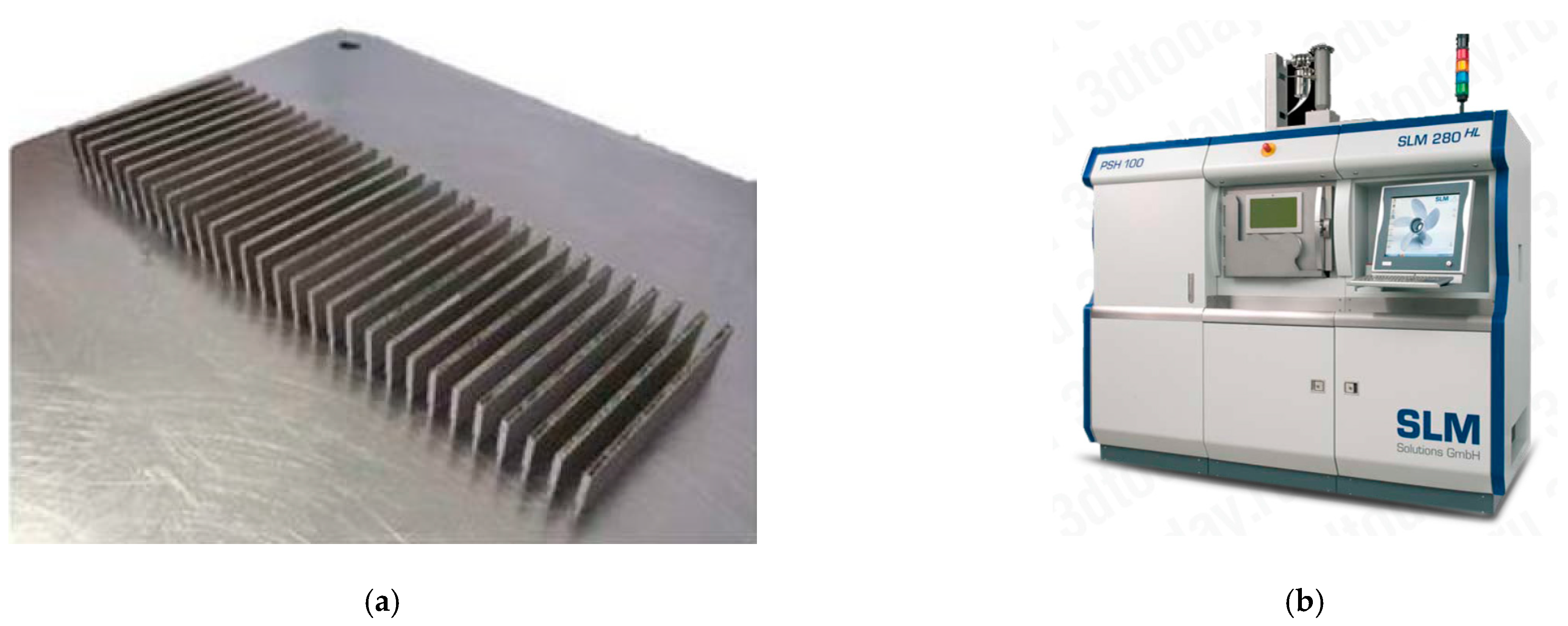
3.2. Materials and Experiment Design
3.3. Solution of the Optimization Problem
FΣ(p,h,v,t) → max
4. Conclusions
- A generalized LP optimization model for determining the technological parameters of LPBF was proposed, containing:
- An objective function in the form of additive normalized performance parameters and one of the key quality characteristics;
- The domain of definition, formed by constraints on the limiting values of the quality characteristics (mechanical properties, surface roughness, parameters of the continuity of the material structure), which were presented as polynomial dependencies of the quality characteristics for technological parameters.
- The initial data for the LP optimization process should be grouped according to the recommended base values of layer thickness (t), scanning speed (v), laser power (P), and hatch spacing (h). The lower and upper limits of deviations from the recommended values were also calculated from Equation (2) and are indicated in the matrix of constraints. The recommended values P, v, h, and t (base point) can be obtained from previous tests or known data.
- The optimization model for determining the technological parameters of LPBF was tested with LPBF specimens from HN58MBYu. The results of the optimization made it possible to determine the optimal technological AM regimes for the formulated objective function and the assigned constraints. Since the area of constraints regarding the variation of technological parameters was rather narrow, this was justified by the use of the chosen optimization method—linear programming. Then, most of the optimal parameters took on the value of constraints. Thus, the optimal scanning speed corresponded to the maximum vopt = vmax = 640 mm/s, which is explained by the requirements of maximum productivity; and the deposited layer thickness was the minimum t = 0.05 mm, which is explained by the requirements of minimizing the roughness. The optimum values of the laser power P = 293 W and hatching step h = 0.14 mm provide a balanced value for the fusion volume energy density E = 65.4 J/mm3, which, according to the data in Table 2, should correspond to the required mechanical properties.
Author Contributions
Funding
Data Availability Statement
Conflicts of Interest
References
- Najmon, J.C.; Raeisi, S.; Tovar, A. 2—Review of additive manufacturing technologies and applications in the aerospace industry. In Additive Manufacturing for the Aerospace Industry; Froes, F., Boyer, R., Eds.; Elsevier: Amsterdam, The Netherlands, 2019; pp. 7–31. Available online: https://www.sciencedirect.com/science/article/pii/B9780128140628000029 (accessed on 10 September 2022). [CrossRef]
- Vora, J.; Parmar, H.; Chaudhari, R.; Khanna, S.; Doshi, M.; Patel, V. Experimental investigations on mechanical properties of multi-layered structure fabricated by GMAW-based WAAM of SS316L. J. Mater. Res. Technol. 2022, 20, 2748–2757. Available online: https://www.sciencedirect.com/science/article/pii/S2238785422013072 (accessed on 10 September 2022). [CrossRef]
- Chen, Z. Understanding of the Modeling Method in Additive Manufacturing. IOP Conf. Ser. Mater. Sci. Eng. 2020, 711, 012017. [Google Scholar] [CrossRef]
- International Organization for Standardization. Additive manufacturing—General principles—Terminology. ISO/ASTM 52900. 2018. Available online: https://www.iso.org/obp/ui/#iso:std:iso-astm:52900:dis:ed-2:v1:en (accessed on 10 September 2022).
- Wang, D.; Liu, L.; Deng, G.; Deng, C.; Bai, Y.; Yang, Y.; Wu, W.; Chen, J.; Liu, Y.; Wang, Y.; et al. Recent progress on additive manufacturing of multi-material structures with laser powder bed fusion. Virtual Phys. Prototyp. 2022, 17, 329–365. [Google Scholar] [CrossRef]
- Yap, C.Y.; Chua, C.K.; Dong, Z.L.; Liu, Z.H.; Zhang, D.Q.; Loh, L.E.; Sing, S.L. Review of selective laser melting: Materials and applications. Appl. Phys. Rev. 2015, 2, 041101. [Google Scholar] [CrossRef]
- Qiu, C.; Al Kindi, M.; Aladawi, A.S.; Al Hatmi, I. A Comprehensive Study on Microstructure and Tensile Behavior of a Selectively Laser Melted Stainless Steel. Sci. Rep. 2018, 8, 1–16. [Google Scholar] [CrossRef] [PubMed] [Green Version]
- Charles, A.; Elkaseer, A.; Thijs, L.; Hagenmeyer, V.; Scholz, S.G. Effect of Process Parameters on the Generated Surface Roughness of Down-Facing Surfaces in Selective Laser Melting. Appl. Sci. 2019, 9, 1256. [Google Scholar] [CrossRef] [Green Version]
- Perevoshchikova, N.; Rigaud, J.; Sha, Y.; Heilmaier, M.; Finnin, B.; Labelle, E.; Wu, X. Optimisation of Selective Laser Melting Parameters for the Ni-Based Superalloy IN-738 LC Using Doehlert’s Design. Rapid Prototyp. J. 2017, 23, 881–892. [Google Scholar] [CrossRef] [Green Version]
- Zhou, Y.; Abbara, E.; Jiang, D.; Azizi, A.; Poliks, M.D.; Ning, F. High-cycle fatigue properties of curved-surface AlSi10Mg parts fabricated by powder bed fusion additive manufacturing. Rapid Prototyp. J. 2022, 28, 7. [Google Scholar] [CrossRef]
- Mani, M.; Lane, B.M.; Donmez, M.A.; Feng, S.C.; Moylan, S.P. A Review on Measurement Science Needs for Real-Time Control of Additive Manufacturing Metal Powder Bed Fusion Processes. Int. J. Prod. Res. 2016, 55, 1–19. [Google Scholar] [CrossRef]
- Baturynska, I.; Semeniuta, O.; Martinsen, K. Optimization of Process Parameters for Powder Bed Fusion Additive Manufacturing by Combination of Machine Learning and Finite Element Method: A Conceptual Framework. Proced. CIRP 2018, 67, 227–232. [Google Scholar] [CrossRef]
- Singh, A.K.; Prakash, R.S. DoE Based Three-Dimensional Finite Element Analysis for Predicting Density of a Laser-Sintered Part. Rap. Prototyp. J. 2010, 16, 460–467. [Google Scholar] [CrossRef]
- Gong, H.; Rafi, K.; Gu, H.; Starr, T.; Stucker, B. Analysis of Defect Generation in Ti–6al–4v Parts Made Using Powder Bed Fusion Additive Manufacturing Processes. Addit. Manufact. 2014, 1, 87–98. [Google Scholar] [CrossRef]
- Thipprakmas, S.; Phanitwong, W. Process Parameter Design of Spring-Back and Spring-Go in V-Bending Process Using Taguchi Technique. Mater. Des. 2011, 32, 4430–4436. [Google Scholar] [CrossRef]
- Giri, N.C.; Das, M.N. Design and Analysis of Experiments; Wiley: New Delhi, India, 1986. [Google Scholar]
- Krishnan, M.; Atzeni, E.; Canali, R.; Calignano, F.; Manfredi, D.G.; Ambrosio, E.P.; Iuliano, L. On the Effect of Process Parameters on Properties of AlSi10Mg Parts Produced by DMLS. Rapid Prototyp. J. 2014, 20, 449–458. [Google Scholar] [CrossRef]
- Linares, J.-M.; Chaves-Jacob, J.; Lopez, Q.; Sprauel, J.-M. Fatigue life optimization for 17-4Ph steel produced by selective laser melting. Rapid Prototyp. J. 2022, 28, 1–16. [Google Scholar] [CrossRef]
- Khaimovich, A.I.; Stepanenko, I.S.; Smelov, V.G. Optimization of Selective Laser Melting by Evaluation Method of Multiple Quality Characteristics. IOP Conf. Ser. Mater. Sci. Eng. 2018, 302, 012067. [Google Scholar] [CrossRef]
- Fanya, A.; Haruman, E.; Mohd Shahriman, A. Optimization of Multi-Objective Taguchi Method for Hybrid Thermochemical Treatment Applied to AISI 316LVM Biological Grade Stainless Steel. In Reference Module in Materials Science and Materials Engineering; Elsevier: Amsterdam, The Netherlands, 2019. [Google Scholar] [CrossRef]
- Nath, R.; Murugesan, K. Optimization of Double Diffusive Mixed Convection in a Bfs Channel Filled with Alumina Nanoparticle Using Taguchi Method and Utility Concept. Sci. Rep. 2019, 9, 1–19. [Google Scholar] [CrossRef] [PubMed] [Green Version]
- Liu, Y.; Liu, C.; Liu, W.; Ma, Y.; Tang, S.; Liang, C.; Cai, Q.; Zhang, C. Optimization of Parameters in Laser Powder Deposition AlSi10Mg Alloy Using Taguchi Method. Opt. Laser Technol. 2019, 111, 470–480. [Google Scholar] [CrossRef]
- Manjunath, B.; Vinod, A.; Abhinav, K.; Verma, S.; Sankar, M.R. Optimisation of Process Parameters for Deposition of Colmonoy Using Directed Energy Deposition Process. Mater. Today Proc. 2020, 26, 1108–1112. [Google Scholar] [CrossRef]
- Yang, B.; Lai, Y.; Yue, X.; Wang, D.; Zhao, Y. Parametric Optimization of Laser Additive Manufacturing of Inconel 625 Using Taguchi Method and Grey Relational Analysis. Scanning 2020, 2020, 1–10. [Google Scholar] [CrossRef]
- Joguet, D.; Costil, S.; Liao, H.; Danlos, Y. Porosity Content Control of CoCrMo and Titanium Parts by Taguchi Method Applied to Selective Laser Melting Process Parameter. Rapid Prototyp. J. 2016, 22, 20–30. [Google Scholar] [CrossRef]
- Dong, G.; Marleau-Finley, J.; Zhao, Y.F. Investigation of Electrochemical Post-Processing Procedure for Ti-6AL-4V Lattice Structure Manufactured by Direct Metal Laser Sintering (DMLS). Int. J. Adv. Manuf. Technol. 2019, 104, 3401–3417. [Google Scholar] [CrossRef]
- Calignano, F.; Manfredi, D.; Ambrosio, E.P.; Iuliano, L.; Fino, P. Influence of Process Parameters on Surface Roughness of Aluminum Parts Produced by DMLS. Int. J. Adv. Manuf. Technol. 2013, 67, 2743–2751. [Google Scholar] [CrossRef] [Green Version]
- Rathod, M.K.R.; Karia, M.M.C. Experimental Study for Effects of Process Parameters of Selective Laser Sintering for alsi10mg. Int. J. Technol. Res. Eng. 2020, 7, 6957–6960. [Google Scholar]
- Jiang, H.-Z.; Li, Z.-Y.; Feng, T.; Wu, P.-Y.; Chen, Q.-S.; Feng, Y.-L.; Li, S.-W.; Gao, H.; Xu, H.-J. Factor Analysis of Selective Laser Melting Process Parameters with Normalised Quantities and Taguchi Method. Opt. Laser Technol. 2019, 119, 105592. [Google Scholar] [CrossRef]
- Campanelli, S.; Casalino, G.; Contuzzi, N.; Ludovico, A. Taguchi Optimization of the Surface Finish Obtained by Laser Ablation on Selective Laser Molten Steel Parts. Proced. CIRP 2013, 12, 462–467. [Google Scholar] [CrossRef]
- Sathish, S.; Anandakrishnan, V.; Dillibabu, V.; Muthukannan, D.; Balamuralikrishnan, N. Optimization of Coefficient of Friction for Direct Metal Laser Sintered Inconel 718. In Advances in Manufacturing Technology; Springer: Berlin/Heidelberg, Germany, 2019; pp. 371–379. [Google Scholar]
- Carley, K.M.; Kamneva, N.Y.; Reminga, J. Response Surface Methodology; Center for Computational Analysis of Social and Organizational Systems: Pittsburgh, PA, USA, 2004; p. 32. [Google Scholar]
- Dada, M.; Popoola, P.; Mathe, N.; Pityana, S.; Adeosun, S. Parametric Optimization of Laser Deposited High Entropy Alloys Using Response Surface Methodology (RSM). Int. J. Adv. Manuf. Technol. 2020, 109, 2719–2732. [Google Scholar] [CrossRef]
- Read, N.; Wang, W.; Essa, K.; Attallah, M.M. Selective Laser Melting of ALSi10Mg Alloy: Process Optimisation and Mechanical Properties Development. Mater. Des. 2015, 65, 417–424. [Google Scholar] [CrossRef] [Green Version]
- Pant, P.; Chatterjee, D.; Nandi, T.; Samanta, S.K.; Lohar, A.K.; Changdar, A. Statistical Modelling and Optimization of Clad Characteristics in Laser Metal Deposition of Austenitic Stainless Steel. J. Braz. Soc. Mech. Sci. Eng. 2019, 41, 283. [Google Scholar] [CrossRef]
- Bartolomeu, F.; Faria, S.; Carvalho, O.; Pinto, E.; Alves, N.; Silva, F.S.; Miranda, G. Predictive Models for Physical and Mechanical Properties of Ti6Al4V Produced by Selective Laser Melting. Mater. Sci. Eng. A 2016, 663, 181–192. [Google Scholar] [CrossRef]
- El-Sayed, M.A.; Ghazy, M.; Youssef, Y.; Essa, K. Optimization of SLM Process Parameters for Ti6Al4V Medical Implants. Rapid Prototyp. J. 2019, 25, 433–447. [Google Scholar] [CrossRef] [Green Version]
- Marmarelis, M.G.; Ghanem, R.G. Data-Driven Stochastic Optimization on Manifolds for Additive Manufacturing. Comput. Mater. Sci. 2020, 181, 109750. [Google Scholar] [CrossRef]
- Fotovvati, B.; Balasubramanian, M.; Asadi, E. Modeling and Optimization Approaches of Laser-Based Powder-Bed Fusion Process for Ti-6Al-4V Alloy. Coatings 2020, 10, 1104. [Google Scholar] [CrossRef]
- Wang, G.; Huang, L.; Liu, Z.; Qin, Z.; He, W.; Liu, F.; Chen, C.; Nie, Y. Process Optimization and Mechanical Properties of Oxide Dispersion Strengthened Nickel-Based Superalloy by Selective Laser Melting. Mater. Des. 2020, 188, 108418. [Google Scholar] [CrossRef]
- Hashmi, S. Comprehensive Materials Finishing; Elsevier: Amsterdam, The Netherlands, 2017; pp. 1–25. [Google Scholar]
- Dongari, S.; Davidson, M.J. Multi response optimization of Inconel 625 wire arc deposition for development of additive manufactured components using Grey relational analysis (GRA). Metallurg. Mater. Eng. 2021, 27, 2. [Google Scholar] [CrossRef]
- Bhadrakali, A.; Narayana, K.; Prabhu, T.; Reddy, Y. Optimization of mechanical properties of ER-4043 specimens fabricated by WAAM process through Grey Relational Analysis. IOP Conf. Ser. Mater. Sci. Eng. 2021, 1055, 012047. [Google Scholar] [CrossRef]
- Khaimovich, A.; Erisov, Y.; Smelov, V.; Agapovichev, A.; Petrov, I.; Razhivin, V.; Bobrovskij, I.; Kokareva, V.; Kuzin, A. Interface quality indices of Al–10Si–Mg aluminum alloy and Cr18–Ni10–Ti stainless-steel bimetal fabricated via selective laser melting. Metals 2021, 11, 172. [Google Scholar] [CrossRef]
- Garg, A.; Lam, J.S.L.; Savalani, M. A New Computational Intelligence Approach in Formulation of Functional Relationship of Open Porosity of the Additive Manufacturing Process. Int. J. Adv. Manufact. Technol. 2015, 80, 555–565. [Google Scholar] [CrossRef]
- Garg, A.; Lam, J.S.L. Measurement of Environmental Aspect of 3-D Printing Process Using Soft Computing Methods. Measurement 2015, 75, 210–217. [Google Scholar] [CrossRef]
- Li, X.-F.; Dong, J.-H.; Zhang, Y.-Z. Modeling and Applying of Rbf Neural Network Based on Fuzzy Clustering and Pseudo-Inverse Method. In Proceedings of the International Conference on Information Engineering and Computer Science (ICIECS), Wuhan, China, 19–20 December 2009; pp. 1–4. [Google Scholar]
- Wang, R.-J.; Li, J.; Wang, F.; Li, X.; Wu, Q. Ann Model for the Prediction of Density in Selective Laser Sintering. Int. J. Manufact. Res. 2009, 4, 362–373. [Google Scholar] [CrossRef]
- Wang, R.-J.; Wang, L.; Zhao, L.; Liu, Z. Influence of Process Parameters on Part Shrinkage in Sls. Int. J. Adv. Manufact. Technol. 2007, 33, 498–504. [Google Scholar] [CrossRef]
- Rong-Ji, W.; Xin-Hua, L.; Qing-Ding, W.; Lingling, W. Optimizing Process Parameters for Selective Laser Sintering Based on Neural Network and Genetic Algorithm. Int. J. Adv. Manufact. Technol. 2009, 42, 1035–1042. [Google Scholar] [CrossRef]
- Negi, S.; Sharma, R.K. Study on Shrinkage Behaviour of Laser Sintered Pa 3200gf Specimens Using Rsm and Ann. Rap. Prototyp. J. 2016, 22, 645–659. [Google Scholar] [CrossRef]
- Munguía, J.; Ciurana, J.; Riba, C. Neural-Network-Based Model for Build-Time Estimation in Selective Laser Sintering. Proc. Inst. Mechan. Eng. Part B J. Eng. Manufact. 2009, 223, 995–1003. [Google Scholar] [CrossRef]
- Shen, X.; Yao, J.; Wang, Y.; Yang, J. Density Prediction of Selective Laser Sintering Parts Based on Artificial Neural Network. In Proceedings of the International Symposium on Neural Networks, Dalian, China, 19–21 August 2004; Springer: Berlin/Heidelberg, Germany, 2004; pp. 832–840. [Google Scholar]
- Murphy, T.; Tsui, K.-T.; Allen, J. A Review of Robust Design Methods for Multiple Responses. Res. Eng. Des. 2005, 15, 201–215. [Google Scholar] [CrossRef]
- Zobaa, A.; Abdel Aleem, S.H.E.; Abdelaziz, A.Y. Classical and Recent Aspects of Power System Optimization; Elsevier: Amsterdam, The Netherlands, 2018. [Google Scholar] [CrossRef]
- Goldak, J.; Chakravarti, A.; Bibby, M. A new finite element model for welding heat sources. Metall. Trans. B 1984, 15, 299–305. [Google Scholar] [CrossRef]
- Lindwall, J.; Pacheco, V.; Sahlberg, M.; Lundbäck, A.; Lindgren, L.-E. Thermal simulation and phase modeling of bulk metallic glass in the powder bed fusion process. Addit. Manufact. 2019, 27, 345–352. [Google Scholar] [CrossRef]
- Khorasani, M.; Ghasemi, A.H.; Leary, M.; Sharabian, E.; Cordova, L.; Gibson, I.; Downing, D.; Bateman, S.; Brandt, M.; Rolfe, B. The effect of absorption ratio on meltpool features in laser-based powder bed fusion of IN718. Opt. Laser Technol. 2022, 153, 108263. [Google Scholar] [CrossRef]


| C | S | P | Mn | Cr | Si | Ni | Fe | Al | B | Mo | Nb | Mg | Y | La |
|---|---|---|---|---|---|---|---|---|---|---|---|---|---|---|
| 0.05 | 0.011 | 0.012 | 0.49 | 26.4 | 0.8 | Balance | 2.7 | 1.29 | 0.002 | 7.6 | 3.1 | 0.02 | 0.02 | 0.03 |
| No. | Energy Density Е, J/mm3 | Laser Power Р, W | Scanning Speed v, mm/s | Scanning Step h, mm | Layer Thickness t, mm | Sample Thickness S, mm | Tensile Strength, MPa | Relative Elongation | Ra |
|---|---|---|---|---|---|---|---|---|---|
| 1 | 56 | 148 | 480 | 0.11 | 0.05 | 3 | 1036 | 21.1 | 4.48 |
| 2 | 69 | 215 | 480 | 0.13 | 0.05 | 2 | 1024 | 19.9 | 4.46 |
| 3 | 76 | 306 | 480 | 0.14 | 0.06 | 2 | 1020 | 16.2 | 4.58 |
| 4 | 63 | 218 | 480 | 0.12 | 0.06 | 3 | 1011 | 24.3 | 4.56 |
| 5 | 56 | 262 | 600 | 0.13 | 0.06 | 3 | 962 | 20.1 | 4.49 |
| 6 | 69 | 273 | 600 | 0.11 | 0.06 | 2 | 1024 | 19.6 | 4.51 |
| 7 | 76 | 274 | 600 | 0.12 | 0.05 | 2 | 1025 | 21.2 | 4.50 |
| 8 | 63 | 265 | 600 | 0.14 | 0.05 | 3 | 1013 | 25.1 | 4.47 |
| 9 | 56 | 259 | 660 | 0.14 | 0.05 | 2 | 1051 | 20.8 | 4.50 |
| 10 | 69 | 273 | 660 | 0.12 | 0.05 | 3 | 1024 | 23.0 | 4.47 |
| 11 | 76 | 331 | 660 | 0.11 | 0.06 | 3 | 998 | 22.5 | 4.48 |
| 12 | 63 | 299 | 660 | 0.12 | 0.06 | 2 | 1013 | 17.3 | 4.52 |
| 13 | 56 | 218 | 540 | 0.12 | 0.06 | 2 | 1055 | 15.9 | 4.59 |
| 14 | 69 | 313 | 540 | 0.14 | 0.06 | 3 | 980 | 19.6 | 4.60 |
| 15 | 76 | 267 | 540 | 0.13 | 0.05 | 3 | 1024 | 23.1 | 4.42 |
| 16 | 63 | 187 | 540 | 0.11 | 0.05 | 2 | 1081 | 19.85 | 4.49 |
| max | 76 | 331 | 660 | 0.14 | 0.06 | 3 | 1081 | 25.1 | 4.6 |
| min | 56 | 148 | 480 | 0.11 | 0.05 | 2 | 962 | 15.9 | 4.42 |
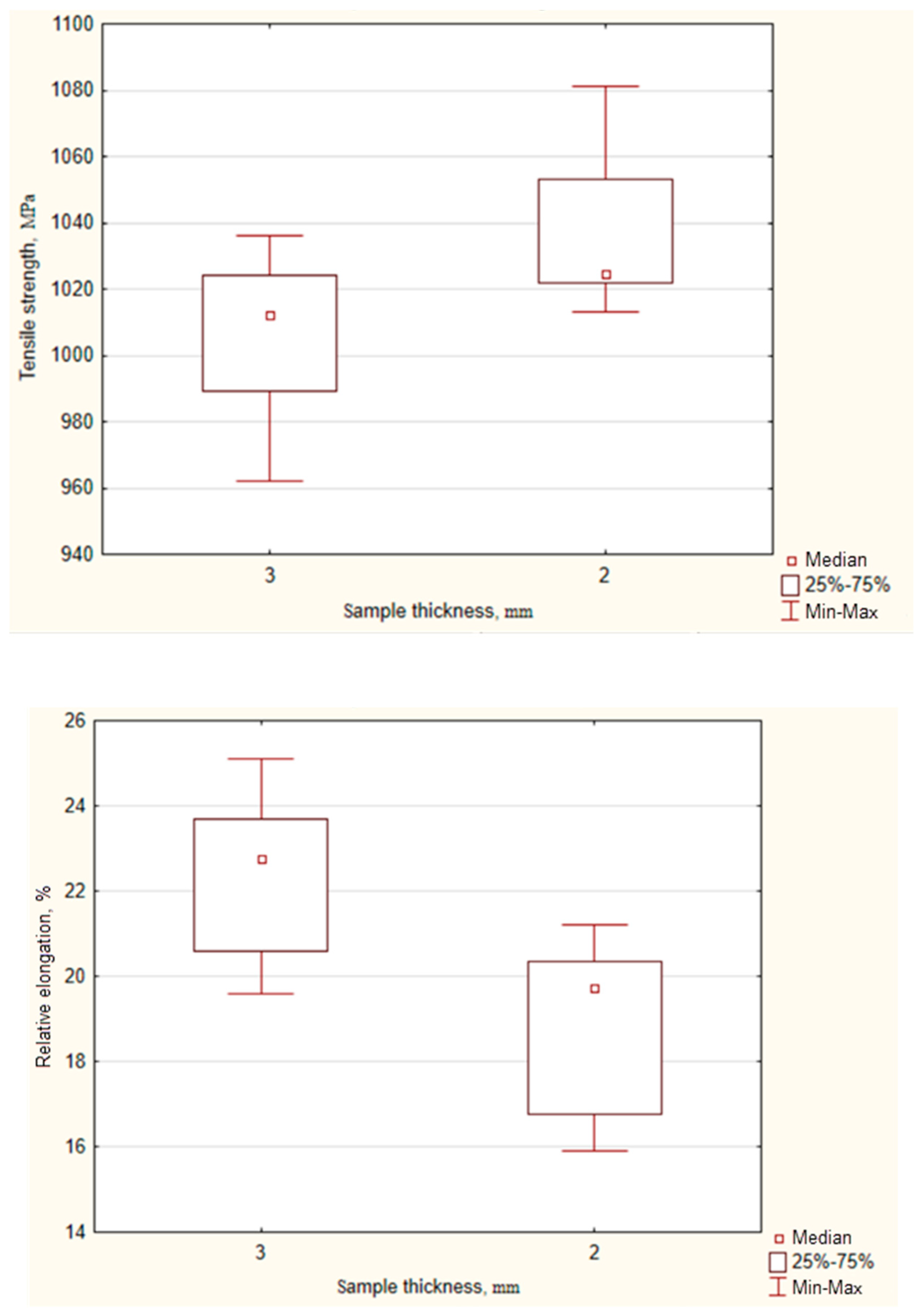
| Mechanical Properties | Mann–Whitney U-Criterion | Z—Normal Distribution Function | p-Level |
|---|---|---|---|
| Tensile strength, MPa | 11.50000 | −2.10042 | 0.035693 |
| Relative elongation, % | 7.50000 | 2.52050 | 0.011719 |
| No. | Logarithm of Linear Power Density, ln(p/v) | Logarithm of Scanning Step, ln(h) | Logarithm of Thickness Layer, ln(t) | Logarithm of Tensile Strength, ln(σ) | Logarithm of Relative Elongation, ln(δ) |
|---|---|---|---|---|---|
| 1 | −1.17657 | −2.20727 | −2.99573 | 6.943122 | 3.049273 |
| 2 | −0.78929 | −2.12026 | −2.81341 | 6.918695 | 3.190476 |
| 3 | −0.82859 | −2.04022 | −2.81341 | 6.869014 | 3.00072 |
| 4 | −0.8172 | −1.96611 | −2.99573 | 6.920672 | 3.222868 |
| 5 | −0.88277 | −2.12026 | −2.99573 | 6.931472 | 3.135494 |
| 6 | −0.69012 | −2.20727 | −2.81341 | 6.905753 | 3.113515 |
| 7 | −0.54537 | −1.96611 | −2.81341 | 6.887553 | 2.97553 |
| 8 | −0.70432 | −2.04022 | −2.99573 | 6.931472 | 3.139833 |
| Input Parameter | Logarithm of Tensile Strength, ln(σ) | Logarithm of Relative Elongation, ln(δ) | ||||
|---|---|---|---|---|---|---|
| Group Dispersion SS | Fisher F-Test | p-Value | SS—Dispersion in Group | Fisher F-Test | p-Value | |
| ln(P/v) | 0.134641 | 9.05307 | 0.019695 | 0.02955 | 2.497524 | 0.158037 |
| ln(h) | 0.255182 | 17.15802 | 0.004337 | 0.07102 | 6.002435 | 0.044108 |
| ln(t) | 0.612845 | 41.20670 | 0.000361 | 0.09798 | 8.280913 | 0.023731 |
| No. | Characteristic | Type | Value |
|---|---|---|---|
| 1 | Yield strength (MPa) | Min | 1020 |
| 2 | Relative elongation | Min | 20 |
| 3 | Layer thickness, t (mm) | Min | 0.05 |
| 4 | Layer thickness, t (mm) | Max | 0.06 |
| 5 | Hatch spacing, h (mm) | Min | 0.1 |
| 6 | Hatch spacing, h (mm) | Max | 0.15 |
| 7 | Laser power, P (W) | Min | 200 |
| 8 | Laser power, P (W) | Max | 300 |
| 9 | Scanning speed, v (mm/s) | Min | 500 |
| 10 | Scanning speed, v (mm/s) | Max | 640 |
| 11 | Roughness, Ra (µm) | Min | 12 |
| 12 | Melting pool depth, c (mm) | Approximately | 0.5 |
| 13 | Hatch spacing, h0 (mm) | Base * | 0.12 |
| 14 | Scanning speed, v0 (mm/s) | Base * | 540 |
| 15 | Layer thickness, t0 (mm) | Base * | 0.06 |
| 16 | Laser power, P0 (W) | Base * | 218 |
| Amin | Amin∙X | Bmin | |||||
| 0.75506 | −0.75506 | −1.44727 | −1.54890 | = | 6.927558 | ≥ | 6.927558 |
| 0.353741 | −0.353741 | −0.763524 | −0.619330 | = | 3.096988 | ≥ | 2.995732 |
| 0 | 0 | 1 | 0 | = | −1.988349 | ≥ | −2.302585 |
| 0 | 0 | 0 | 1 | = | −2.995732 | ≥ | −2.995732 |
| 1 | 0 | 0 | 0 | = | 5.679789 | ≥ | 5.298317 |
| 0 | 1 | 0 | 0 | = | 6.461468 | ≥ | 6.214608 |
| −1 | 1 | 1 | 1 | = | −4.202402 | ≥ | −4.202402 |
| Amax | Amax∙X | Bmax | |||||
| 0 | 0 | 0 | 0.075 | = | 1.258208 | ≥ | 2.484907 |
| 0 | 0 | 1 | 0 | = | −1.988349 | ≥ | −1.89712 |
| 0 | 0 | 0 | 1 | = | −2.995732 | ≥ | −2.813411 |
| 1 | 0 | 0 | 0 | = | 5.679789 | ≥ | 5.703782 |
| 0 | 1 | 0 | 0 | = | 6.461468 | ≥ | 6.461468 |
| −1 | 1 | 1 | 1 | = | −4.202402 | ≥ | −4.0266 |
| Xopt | |||
|---|---|---|---|
| ln(P) | ln(v) | ln(h) | ln(t) |
| 5.679788803 | 6.461468176 | −1.988349345 | −2.995732274 |
| Laser Power, Р (W) | Scanning Speed, v (mm/s) | Scanning Step, h (mm) | Layer Thickness, t (mm) |
|---|---|---|---|
| 293 | 640 | 0.14 | 0.05 |
Publisher’s Note: MDPI stays neutral with regard to jurisdictional claims in published maps and institutional affiliations. |
© 2022 by the authors. Licensee MDPI, Basel, Switzerland. This article is an open access article distributed under the terms and conditions of the Creative Commons Attribution (CC BY) license (https://creativecommons.org/licenses/by/4.0/).
Share and Cite
Khaimovich, A.; Balyakin, A.; Oleynik, M.; Meshkov, A.; Smelov, V. Optimization of Process Parameters for Powder Bed Fusion Additive Manufacturing Using a Linear Programming Method: A Conceptual Framework. Metals 2022, 12, 1976. https://doi.org/10.3390/met12111976
Khaimovich A, Balyakin A, Oleynik M, Meshkov A, Smelov V. Optimization of Process Parameters for Powder Bed Fusion Additive Manufacturing Using a Linear Programming Method: A Conceptual Framework. Metals. 2022; 12(11):1976. https://doi.org/10.3390/met12111976
Chicago/Turabian StyleKhaimovich, Alexander, Andrey Balyakin, Maxim Oleynik, Artem Meshkov, and Vitaly Smelov. 2022. "Optimization of Process Parameters for Powder Bed Fusion Additive Manufacturing Using a Linear Programming Method: A Conceptual Framework" Metals 12, no. 11: 1976. https://doi.org/10.3390/met12111976