Multialgorithm Fusion for Milling Tool Abrasion and Breakage Evaluation Based on Machine Vision

Abstract

Aiming at the problem that the current tool status monitoring system cannot measure the area of the abrasion and breakage from the milling tool images at the same time, a new detection fusion method for milling tool abrasion and breakage based on machine vision is proposed. This method divides the milling tool status into abrasion and breakage. The abrasion is recognized by an adaptive region localization growing method, and the breakage is recognized by an edge fitting reconstruction method based on distance threshold. Then, the area of tool damage can be accurately measured based on the identified abrasion and breakage information. Experiments show that the proposed method could effectively detect both the tool abrasion and breakage, and provide a better monitoring effect than that of the conventional method that only considers tool abrasion status. The proposed approach was verified by the experimental results, and the accuracy of the tool damage area characteristic was over 95%.

1. Introduction

The milling process has outstanding performance both in general material processing and complex three-dimensional surface processing. However, due to the high-speed discontinuous cutting characteristics, the tool will wear out easily. The worn or broken tool directly affects the machined quality of the product. In the meantime, severely worn tools can cause breakage, chatter, etc., which can damage the machine. Therefore, effective tool wear and damage monitoring are quite meaningful.

Recently, detection methods based on machine vision have been widely studied for milling tool status monitoring and machining process monitoring. Machine vision systems consist of image sensors, image processing algorithms, and pattern recognition tools. The tool monitoring system based on machine vision uses visual equipment to extract the physical properties of the tool, such as brightness, texture, color, pixel spatial distribution, etc., and transmit and process digital images to realize the monitoring and control of the equipment. Through reasonable matching, the machine vision can realize high-precision monitoring of the processing and improve the flexibility and automation of production. Moreover, it can easily realize machine vision automation and software integration, which forms the basis of intelligent manufacturing. Machine vision systems are widely used in manufacturing and metal surface defect monitoring [1,2], metal additive manufacturing monitoring [3,4], manufacturing process assembly and control [5], etc.

According to the milling tool wear mechanism, the worn form still mainly manifests as the breakage of the tool tip [6]. Wiederkehr [7] introduced and discussed the idea of self-optimizing machining systems (SOMS). A technology based on machine vision could be integrated into SOMS in order to optimize productivity, quality, and efficiency in manufacturing. Zhu [8] proposed a region-growing algorithm based on morphological component analysis, which could effectively suppress the interference of background and noise, and extract the worn region of the target tool image. Dai [9] proposed a machine vision system specifically for milling cutters, which could be used for progressive wear detection. The control system drove the machine vision 3D motion platform, which could detect and capture images in focus within a given processing time. Li [10] proposed a novel two-dimensional tool wear estimation method and combined other signal features to estimate the tool wear area, which improved the model practicability of the revised paper. Fernandez-Robles [11] designed three methods, including morphological operations, k-means clustering, and the Otsu multilevel algorithm, to test the effects in three tool views, respectively. The test results indicated that the worn prediction value could provide valuable information for determining the extent of tool wear. Yu [12] used the local threshold variance to obtain the tool contour and the adaptive contrast enhancement algorithm based on two-dimensional local mean decomposition (BLMD) to realize the tool wear area acquisition. Yu [13] proposed a nonlocal mean denoising method based on the integral image and Turky dual-weight kernel function. This method could effectively complete the detection and boundary extraction of the tool wear area. Hou [14] proposed a self-matching algorithm, which used the worn tool itself as a reference object to detect tool wear. It provided an idea for the acquisition of damaged areas. Li [15] discovered the association principle between the change law of the cutting edge grayscale and the relative position of the original and worn boundary, which was used to establish the probability functions to accurately reconstruct the curved original tool boundary via Bayesian inference. Marei [16] developed a transfer learning-enabled convolutional neural network (CNN) approach to predict the health state of cutting tools. The results indicated the suitability of the developed approach, particularly with ResNet-18, for estimating the wear width of cutting tools. Bergs [17] proposed a deep learning approach in order to quantify the tool wear state for semantic segmentation trained on individual tool type datasets (ball and mill, end mill, drills and inserts). Even though this method could satisfy different tool types, the test data still needed to be labeled as accurately as possible, and the intersection over union (IOU) coefficient was not at a high level. Ye [18] proposed a high-precision visual detection method of tool damage based on visual feature migration and edge reconstruction, which detected tool damage area by wear area and breakage area. However, the experimental images in this paper were not obtained in the actual machine tool environment, and the experimental results were not comprehensive. It was a major limitation. An analysis of papers in recent years indicates that the current research on milling focuses on abrasion and breakage, respectively, but the number of papers on the combination of both statuses are few. Moreover, some methods were only tested on the experimental platform and could not be applied to practical manufacturing. It is important to carry out research on the quantitative analysis of tool status to achieve accurate monitoring of tool status from machine tool images.

In this paper, the milling tool status was divided into two statuses, i.e., the abrasion and the breakage. The area of abrasion could guide the process status information of the tool, and the area of breakage could guide the critical status information of the tool. These tool statuses could provide a more accurate reference for the monitoring of milling tools.

The technical flowchart of this paper is shown in Figure 1. First, the original images were denoised with a median filter; next, two operations were performed on the denoised images to determine the abrasion and breakage of the milling tool, separately. For the abrasion, the adaptive region localization located the abrasion initially, and then the region-growing algorithm could obtain the abrasion. In terms of the breakage, the image presegmentation processing was performed by the Sobel + Otsu approach, and the breakage area was obtained by edge fitting reconstruction. The monitoring results were the area value of the abrasion and breakage obtained in the above steps.

2. Image Acquisition System

2.1. Hardware Equipment

The machine vision acquisition system consists of a CMOS camera, a telecentric lens, a ring light source, and a camera light source clamping platform. A monochromatic camera mainly uses the grayscale information of the image to reflect the tool status. Figure 2 shows the image acquisition system. The camera and the light source are locked on the bracket platform by screws, which ensures the good stability of the camera and the coaxiality of the light source. At the same time, the ring light source should be placed in front of the tool to provide excellent lighting conditions. The appropriate incident angle and light intensity of the light source can be adjusted through the sliding table structure. Based on the above device, the images of the tool can be obtained and transmitted to the computer platform with Gigabit Ethernet. The main parameters of the equipment are listed in

Table 1. Parameter diagram of machine vision equipment.

Equipment	Parameter
Industrial camera (MA-CA050-12GC)	Resolution: 2448 × 2048; Chart size: 2/3″
Lens (DH110-4F28X)	Magnification: 4.0×; Depth of field: 0.3 mm
LED light source (MV-R6660S-W)	Power: 6.7 W; Angle: 60°; Color temperature: 6000–10,000 k

.

2.2. Tool Cutting Sequence

Figure 3 shows the cutting sequence of the tool. An image dataset was captured after every cutting, and the 15th cutting tool means the image was captured after the 15th cutting in the processing. This demonstrates that the tool is gradually worn in the cutting process. In the magnified image of the tool tip, there is a local bright area at the tool tip, which is the reflection of the incident light by the abrasion area of the tool tip. The reflected light ability of the abrasion is stronger than that of the unworn area of the tool, so the abrasion appears as a small bright area compared to other areas. Figure 3b,c show the phenomenon of the tool tip breakage, and it appears as a fracture. These two phenomena, referred to as the abrasion and breakage, exist in the milling process. In this paper, tool abrasion and tool breakage can be regarded as a process quantity and critical quantity in the process of milling, respectively. Therefore, both tool abrasion and breakage should be extracted to monitor the tool status. The schematic diagram of the abrasion and the breakage is shown in Figure 4.

3. Visual Inspection of Tool Abrasion and Breakage

3.1. Extract Tool Abrasion

3.1.1. Image Grayscale Curve Analysis

Tool image shows that the abrasion area appears as a small bright spot in the experimental images, while the background or unworn area is much darker than is the abrasion. According to the analysis of the tool image, the tool image is composed of three parts: the abrasion, the unworn area, and the background area. In order to analyze the distribution of the gray value in each region of the tool image, a marked line along the y-axis is made at a certain point of the abrasion, with the marked line running through the height of the entire image. All the pixel grayscale information of the marked line is recorded. The length of the marked line is the x-axis, and the grayscale value of the marked line is the y-axis. The column pixel grayscale curve distribution diagram is shown in Figure 5. It can be observed that the grayscale value distribution of the image has the following regularity through the pixel grayscale curve: the grayscale value of the abrasion is much higher than that of the unworn area and the background area.

The grayscale distribution trend between each column in the abrasion is the same, and the abrasion is concentrated in a range of larger grayscale value, which indicates similarity. However, for each column, there is the maximum grayscale value. Each column has its threshold, which indicates the characteristic.

3.1.2. Adaptive Region Localization of Abrasion

According to the distribution of the grayscale curve above, the characteristic of the grayscale law can be utilized to automatically identify the location of the abrasion. The suspicious area is found by searching for a suitable threshold to preliminarily locate the region of the abrasion.

• The column pixel grayscale distribution curve of the original grayscale image is counted to calculate the maximum grayscale value of each column of grayscale curves, and the maximum grayscale values of each column of grayscale curves are summed. Then, the summed value are divided by the total number of columns to obtain the final grayscale mean. The grayscale mean value obtained by this operation is taken as the screening threshold, which is expressed as
  $$Va{l}_{\mathrm{area}}=\frac{{{\displaystyle \sum }}_{i=0}^N{G}_{\mathrm{i}}}{N}$$

  (1)

  where i represents the specific number of columns of the image, N is the total number of columns, and G_i is the maximum grayscale value of the column.
  The obtained screening threshold is used as the threshold for image binarization, and the grayscale information of the grayscale image is divided into two regions. Finally, a binarized image of preliminary region localization is obtained, as shown in Figure 6a. The blue line is the contour of the original tool.
• Since the tool abrasion is mainly concentrated on both sides of the tool tip, it is only necessary to further locate the area at the left and right ends to filter out the useless area. Taking the left side as an example, the first nonzero pixel point at the upper left can be obtained by row pixel scanning, denoted as Pixel(x_l,y_l). Then, a circular area is obtained with the center point Pixel(x_l,y_l) and the radius k, where k is the artificially set width limit, and the value of k can refer to the actual geometric limit of abrasion and breakage. In this paper, k is equal to 360 pixels. The final initial location of the abrasion must be within the entire circular area. The right side is processed in a similar way. The final positioning rendering of the abrasion is shown in Figure 6b.

3.1.3. Extraction of Abrasion Based on Region Growing Algorithm

In paper [6], the original tool wear image was decomposed into a target tool image, background image, and noise image via introducing the morphological component analysis (MCA) algorithm. However, if the appropriate equipment and reasonable lighting condition could be established, a better image could also be obtained as well. The tool abrasion images taken by the existing equipment had the characteristics of obvious wear areas and less background noise interference, and similar areas could be easily extracted. The basic principle of the region-growing algorithm is to extract the image region with a certain similar characteristic, and this characteristic is consistent with the above-mentioned similarity of the grayscale curve distribution. Through reasonable growing conditions to express the similarity of the grayscale curve, the entire abrasion can be extracted.

With the abrasion being initially located, the complete abrasion can be extracted by setting the corresponding regional growing conditions. This paper mainly uses the onedged distribution of the abrasion to design the growing conditions. The process can be divided into the following steps:

• By determining the centroid of each abrasion, the average grayscale value of the centroid eight neighborhood is taken as the average threshold, which can be listed as
  $$avervalue=\frac{{{\displaystyle \sum }}_{i=1}^9{g}_{\mathrm{i}}}{9}$$

  (2)

  where g_i is the grayscale value of the centroid point and eight neighborhood.
• A difference with the average threshold by finding the maximum and minimum grayscale values of each abrasion is calculated, and the largest difference is chosen as the final difference difvalue.
• The upper bound of the threshold and lower bound of the threshold are defined as

  $$threshol{d}_{\mathrm{up}}=avervalue+difvalue$$

  (3)

  $$threshol{d}_{\mathrm{low}}=avervalue+difvalue$$

  (4)

By choosing the maximum difference, the growing conditions can be guaranteed to be within the maximum variability.

According to Ahlem Melouah [19], the selection of the seed point position has an important influence on the effect of region growth, and the best seed point position is the center of the segmented region. The center of the region of abrasion is set as the seed growing start point.

In summary, the seed point of the region-growing algorithm designed in this paper is the center of the abrasion, and the upper and lower bounds of the region-growing conditions are dynamically controlled by threshold_up and the threshold_low. The final growing effect is shown in Figure 7.

3.2. Extracting the Tool Breakage

3.2.1. Image Presegmentation of Breakage

Tool breakage mainly manifests as a fracture in the tool tip, while the tool materials are lost and cannot be directly obtained. Hence, the tool edge fitting reconstruction method is adopted to obtain the breakage. In terms of the obtained image, it has blurred edges, low contrast, and interference of the background artifact, as shown in Figure 8. The Otsu segmentation method cannot obtain the ideal segmentation result, and the information of the artifact is inevitably retained, which causes considerable interference to the detection of edge. The above approach is not conducive to edge fitting. This paper proposes a preprocessing method combining the Sobel and Otsu methods.

The Sobel operator is a discrete differential operator used for edge detection, which has good antinoise performance and accurate edge location. The Sobel operator template is defined as follows:

$$d_{\mathrm{x}}=\left[\begin{array}{ccc}-1& 0& 1\\ -2& 0& 2\\ -1& 0& 1\end{array}\right]d_{\mathrm{y}}=\left[\begin{array}{ccc}-1& -2& -1\\ 0& 0& 0\\ 1& 2& 1\end{array}\right]$$

(5)

The Sobel edge detection operator has a good elimination effect on the gradient onedged area with little change in grayscale level. The effect is expressed as follows:

$$\left[\begin{array}{ccccc}100& 101& 102& 103& 150\\ 100& 101& 102& 103& 150\\ 100& 101& 102& 103& 150\\ 100& 101& 102& 103& 150\end{array}\right]\ast \left[\begin{array}{ccc}-1& 0& 1\\ -2& 0& 2\\ -1& 0& 1\end{array}\right]=\left[\begin{array}{ccc}8& 8& 192\\ 8& 8& 192\end{array}\right]$$

(6)

The Sobel operator only processes the middle 6 pixels, and the edge background artifact can be regarded as a series of 100, 101, 102, and 103 adjacent values, with 150 as the edge point. After processing with the Sobel operator, the value of the artifact is converted to lower values, while the edge information remains at higher values. With the preprocessing operation, the interference of background artifact can be effectively reduced, and the edge information can be effectively preserved.

The Otsu approach is a fast and effective binary classification method, and it is used on the results of the Sobel operator. Since the artifact and edge have been further distinguished by the preprocessing of the Sobel approach, the Otsu method can be used to separate images of foreground and background. The final result of the Sobel + Otsu method is shown in Figure 9.

3.2.2. Least-Squares Method

The previous section describes how the presegmentation operation of the breakage is obtained and how the breakage is then extracted by edge fitting reconstruction. It mainly involves the extraction of the edge points and the selection of fitting methods. The extraction of edge points is obtained by pixel scanning, and the fitting method selects high-order algebraic polynomial fitting. According to the idea of regression analysis, any data point can be represented by a curve, which can be described by a high-order algebraic polynomial:

$$f\left(x\right)=a_0+a_{1}x+a_2{x}^2+\cdots \cdots +a_{\mathrm{n}}{x}^n$$

(7)

where a₀, a₁, a₂, and a_n are all constants.

However, the curve through each point is meaningless, since it cannot guarantee that the edge point of the segmentation is the accurate point. The approach of scanning through pixels will inevitably contain wrong edge points. Moreover, the curve through each point cannot represent the true correlation between y and x. Only the curve that conforms to the reasonable trend of the data points is the reasonable boundary.

The least-squares method is an idea used for linear regression. Its core idea is to minimize the sum of squares of the errors, and the estimated model is the closest to the real situation (the error is the true value minus the theoretical value). The fitting curve should be satisfied with Formula (8).

$$Min{\displaystyle \sum }_i^m{(y_{\mathrm{i}}-f\left(x_{\mathrm{i}}\right))}^2$$

(8)

(x_i, y_i) represents the true value of the observation, m is the number of the data point, and f(x) is the constructed fitting function.

The optimal fitting curve that satisfies the current data can be obtained by the least-squares method. Assuming that there are m samples and the fitted curve is a univariate polynomial of degree n, all sample points are substituted into Formula (9):

$$\begin{array}{l}{h}_1=a_0+a_1{x}_1+a_2{x}_1^2+\cdots +a_{\mathrm{n}}{x}_1^n\\ h_2=a_0+a_1{x}_2+a_2{x}_2^2+\cdots +a_{\mathrm{n}}{x}_2^n\\ ⋮\\ h_{\mathrm{m}}=a_0+a_1{x}_{\mathrm{m}}+a_2{x}_{\mathrm{m}}^2+\cdots +a_{\mathrm{n}}{x}_{\mathrm{m}}^n\end{array}$$

(9)

where x₀ = 1 and can be represented by the following matrix:

$$h\left(x\right)=X\theta$$

(10)

where h(x) is a vector of m × 1 representing the theoretical value of the model, θ is a vector of n × 1, and X is a matrix of m × n dimensions. The objective loss function is constructed as follows:

$$J\left(\theta \right)=\frac{1}{2}{||h-Y||}^2=\frac{1}{2}{||X\theta -Y||}^2=\frac{1}{2}{(X\theta -Y)}^T\left(X\theta -Y\right)$$

(11)

Y is the output value of the sample, which is an m × 1 vector.

The principle of least-squares needs to minimize the loss function. The analytical solution to θ can be obtained by taking the derivative of this loss function concerning θ and making it equal to 0, which can be expressed as follows:

$$\frac{\partial }{\partial \theta }J\left(\theta \right)=X^T\left(X\theta -Y\right)=0$$

(12)

$$\theta ={\left(X^{T}X\right)}^{-1}{X}^{T}Y$$

(13)

The obtained θ is the optimal solution of the current fitting function. The fitting function is as follows:

$$f\left(x\right)={\theta }_0+{\theta }_{1}x+{\theta }_2{x}^2+\cdots \cdots +{\theta }_{\mathrm{n}}{x}^n$$

(14)

3.2.3. Technical Route of Breakage

After the previous image is obtained through image presegmentation based on the Sobel + Otsu method and the high-order polynomial fitting method based on the least-squares method, the technical route steps of obtaining the breakage are as follows:

• Pixel scanning is performed on the straight edge and the curved edge of the tool tip to obtain the edge pixel. The coordinates of the pixel point p(x_i,y_i) are recorded, where I = 1, 2,…n.
• A curve fitting is performed based on the existing pixel points. According to the tool shape analysis, the shape of the tool edge is an arc. A high-order polynomial fitting should be selected instead of a first-order polynomial fitting. In the meantime, it can be seen from Figure 10 that an inflection has already appeared during the fitting of the 3^rd-order polynomial. The higher-order polynomial is not suitable for fitting the tool tip arc, and the fitting effect of the 2^nd-degree polynomial is close to the edge shape of the tool tip. The quadratic polynomial fitting C(x) is selected to fit the tool tip arc. However, the curve direction is wrong. The straight edge of the tool tip is fitted with a first-order polynomial S(x). The fitting function is defined as follows:

  $$C\left(x\right)=c_0+c_{1}x+c_2{x}^2$$

  (15)

  $$S\left(x\right)=s_0+s_{1}x$$

  (16)

  where c₀, c₁, c₂, s₀, and s₁ are all constant coefficients.
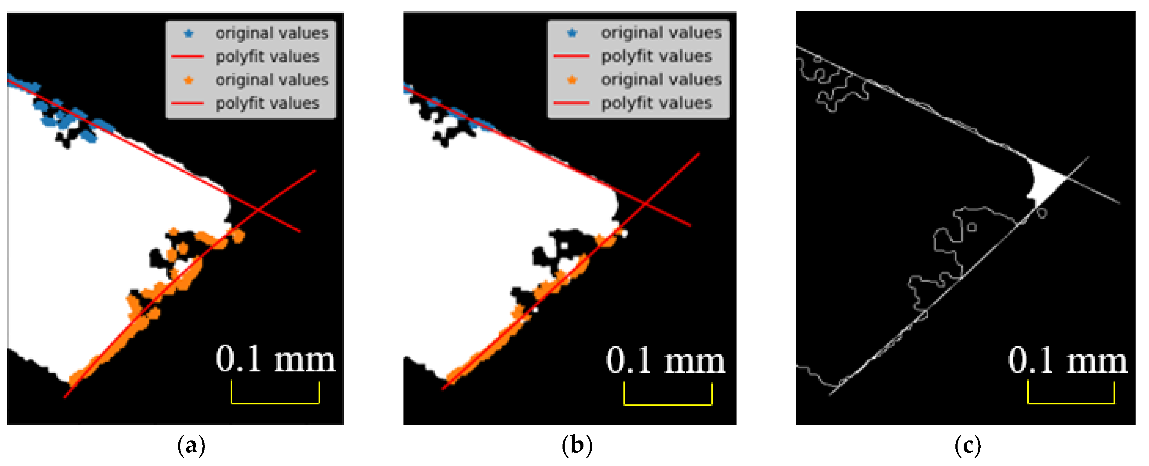
• Error points are eliminated based on the distance threshold. The current fitted edge function can be linearly regressed from the data points by the least-squares method. However, due to the accuracy of image presegmentation, the wrong edge points will inevitably be extracted by scanning edge pixels. In the case of many obvious wrong points, a best-fit curve does not necessarily exist. In this paper, based on the inclusion of wrong points, a method for eliminating error edge points based on the distance threshold is proposed. The idea of this method is as follows:
  Firstly, it is necessary to ensure that more than half of the edge points are correct. In the case of including error points, the first curve fitting is performed as shown in Figure 11a, and the direction of the curve is to the right.
  Secondly, by calculating the closest distance from an edge pixel point to all points of the fitted curve, the closest distance is expressed as

  $$di{s}_{\min }\left(i\right)=min||p\left(x_{\mathrm{I}},y_{\mathrm{i}}\right)-f_1\left(x_{\mathrm{j}},y_{\mathrm{j}}\right)||$$

  (17)

  where p(x_i,y_i) is the edge pixel point, f(x_j,y_j) is the pixel point of the fitted curve, and n is the number of points that make up the fitted curve.
  Finally, the sum of the closest distances is calculated, and the average is obtained. The average distance is used as a distance threshold, which can be shown as

  $$di{s}_{\mathrm{aver}}={\displaystyle \sum }_{i=1}^{m\sum }\frac{di{s}_{\min }\left(i\right)}{m}$$

  (18)

  where m is the number of edge pixel points.
  The distance threshold can reflect the deviation of the edge pixel points from the current fitting curve. The wrong edge pixel points are those data points that seriously deviate from the ideal fitting curve, as shown in Figure 11. As the distance is greater than the threshold, the points are eliminated.
• After the error points are eliminated, the straight edge of the tool is fitted with a straight line, and the curved edge of the tool is fitted with a quadratic polynomial. The fitting effect and the breakage are shown in Figure 11b,c. It demonstrates that the fitted edge is oriented to the left, which is in line with the actual edge trend.

3.3. Monitoring Results of Abrasion and Breakage

The previous two sections describe how the abrasion and breakage of the tool can be obtained, respectively. This section outlines how the abrasion and breakage of the tool can be combined for analysis. Figure 12 shows that the region marked 1 is the breakage, and the rest is the abrasion. This demonstrates that both the abrasion and the breakage have different spatial information, which is an important factor for evaluating the status of the tool. It is inaccurate to evaluate the status of the tool only by a single tool status. It is necessary to monitor the tool status by combining the abrasion and breakage in the process of monitoring the machining of high-precision milling tools.

4. Experiment Analysis

4.1. Pixel Size Standard

Dimensional measurement is an important part of tool abrasion and breakage monitoring. Take an image of a ruler with an industrial camera with the same magnification, all accessories and parameter information of the camera are the same as the conditions when the tool image is acquired.

The minimum scale of the ruler image is 0.1 mm, and the length of 0.1 mm in the image contains 120 pixels which can be measured by pixel measurement software. The unit pixel length, the unit pixel area, and the real area of the abrasion and breakage can be expressed by formulas (19)–(21), respectively,

$$L=\frac{100\mu m}{120}=0.833\mu m$$

(19)

$$A={\left(\frac{100\mu m}{120}\right)}^2=0.694\mu m^2$$

(20)

$$area=A\cdot are{a}_{\mathrm{pixel}}$$

(21)

where L is the unit pixel length, A is the unit pixel area, and area_pixel represents the pixel’s number of area.

4.2. Experimental Setup

There are many indicators to describe the current machining information [20,21,22,23]. However, for the milling process, many papers and standards do not have a clear statement on the optimal index to reveal the machining information of milling tools. Since area is being increasingly used in the tool monitoring of milling [7,8,9] and has an excellent expression ability [24], this paper compares the abrasion and breakage areas extracted by the algorithm with the actual measured areas.

To verify the effectiveness of the multialgorithm fusion proposed in this paper, 14 sets tests were carried out, with grooves being milled with seven tools to different extents of abrasion and breakage status. The experimental tool was an uncoated tungsten steel tool with a diameter of 2 mm, and the workpiece material was STAVAX die steel. The spindle speed was 16,000 rpm, the feed speed 240 mm/min, and the axial cutting depth 0.1 mm/min. After each machining, the tool was blown off with an air gun. All the tool images were captured in the actual machine tool environment.

4.3. Experimental Results and Discussion

Figure 13 shows the experimental results of the tool morphology, in which #1 represents the first experimental tool, and so on. Figure 13a,c show the actual image of the left and right corners of the milling tool, respectively; Figure 13b,d show the abrasion and breakage of the left and right corners of the milling tool extracted by the algorithm in this paper, respectively. For each experimental result, the abrasion and breakage of the tool were extracted. Moreover, the boundary of the extracted area was clear, and there was little interference from background factors. The results indicate that it is reasonable to reflect the status of the tool in terms of the abrasion and breakage in different tools with different extents of abrasion and breakage.

The comparisons of results are shown in

Table 2. Breakage result.

Experience Num	Area (Our Method) (μm2)	Area (Measurement) (μm2)	Accuracy (%)
1(b)	1356.25	1341.66	98.9
1(d)	582.63	556.94	95.6
2(b)	836.11	840.27	99.5
2(d)	631.94	604.82	95.7
3(b)	1465.27	1504.85	97.4
3(d)	686.11	688.19	99.7
4(b)	1758.22	1780.44	98.8
4(d)	1586.70	1524.90	96.1
5(b)	1109.72	1127.78	98.4
5(d)	4086.78	4161.08	98.2
6(b)	2227.07	2202.07	98.8
6(d)	3472.22	3506.25	99.0
7(b)	3813.17	3960.39	96.3
7(d)	4668.72	4768.86	97.9

and

Table 3. Abrasion result.

Experience Num	Area (Our Method) (μm2)	Area (Measurement) (μm2)	Accuracy (%)
1(b)	2143.61	2215.14	96.8
1(d)	1596.43	1533.24	96.1
2(b)	1861.69	1885.99	98.7
2(d)	1874.88	1863.08	99.3
3(b)	1923.49	2001.95	96.1
3(d)	2249.86	2308.19	97.5
4(b)	4029.60	3878.92	96.3
4(d)	2733.16	2724.83	99.7
5(b)	2270.68	2228.33	98.1
5(d)	849.25	806.89	95.1
6(b)	3214.38	3283.12	98.0
6(d)	599.96	598.57	99.8
7(b)	3264.37	3237.29	99.1
7(d)	709.68	756.20	97.3

. The second column is the area value obtained by our algorithm, and the third column is the actual measured area value. The area value obtained by our algorithm was calculated by the function of opencv through calculating the number of area pixels. The actual measured area was calculated with the “Labelme” tool (3.16.2, MIT, USA) to complete the manual cutout. The area value contained two-dimensional size information, which had richer feature information and more drastic changes. The accuracy of the algorithm reached higher than 95%, and the average accuracy reached higher than 97.8%. The accuracy could meet the needs of actual production, and the relatively intact abrasion and breakage of the tool could be successfully obtained. The experimental results indicate that the detection fusion method proposed in this paper can indeed automatically and effectively identify the abrasion and breakage of the tool. This method solves the problem that the current tool status monitoring system has difficulties in automatically identifying the location of the tool abrasion and breakage and accurately measuring the area of tool abrasion and breakage from the collected tool images at the same time.

5. Conclusions

Tool status monitoring is of great significance to ensuring machining quality, improving production efficiency, and reducing the cost the manufacturing. In this paper, the tool status is divided into the tool abrasion extracted by adaptive region localization growing and the tool breakage extracted by distance-threshold-based edge fitting reconstruction. The experiment results indicated that the proposed method had good performance in evaluating the milling tool status. The accuracy of the algorithm could reach more than 95%, and the average accuracy could reach more than 97.8%, which could meet the needs of actual production. Since the tests in this paper were carried out in the actual processing environment, the proposed algorithm could be applied in the actual processing environment. The research results in this paper can provide effective technical support for tool status monitoring in the future. It is worth mentioning that the proposed method has a strong dependence on the lighting environment. Future work can be carried on the improvement of the hardware equipment or image preprocessing for lighting inhomogeneity.

References

1. Luo, Q.; Fang, X.; Liu, L.; Yang, C.; Sun, Y. Automated visual defect detection for flat steel surface: A survey. IEEE Trans. Instrum. Meas. 2020, 69, 626–644. [Google Scholar] [CrossRef] [Green Version]
2. Ren, R.; Hung, T.; Tan, K.C. A generic deep-learning-based approach for automated surface inspection. IEEE Trans. Cybern. 2017, 48, 929–940. [Google Scholar] [CrossRef] [PubMed]
3. Scime, L.; Beuth, J. Anomaly detection and classification in a laser powder bed additive manufacturing process using a trained computer vision algorithm. Addit. Manuf. 2018, 19, 114–126. [Google Scholar] [CrossRef]
4. Aminzadeh, M.; Kurfess, T.R. Online quality inspection using Bayesian classification in powder-bed additive manufacturing from high-resolution visual camera images. J. Intell. Manuf. 2019, 30, 2505–2523. [Google Scholar] [CrossRef]
5. Chauhan, V.; Surgenor, B. Fault detection and classification in automated assembly machines using machine vision. Int. J. Adv. Manuf. Technol. 2017, 90, 2491–2512. [Google Scholar] [CrossRef] [Green Version]
6. Zhao, Y.; Liang, Y.; Bai, Q.; Wang, B. Experimental study on micro-milling machine, micro-tool wear and cutting force in micromachining. Opt. Precis. Eng. 2007, 15, 894–902. [Google Scholar]
7. Möhring, H.C.; Wiederkehr, P.; Erkorkmaz, K.; Kakinuma, Y. Self-optimizing machining systems. CIRP Ann. 2020, 69, 740–763. [Google Scholar] [CrossRef]
8. Zhu, K.; Yu, X. The monitoring of micro milling tool wear conditions by wear area estimation. Mech. Syst. Signal Process. 2017, 93, 80–91. [Google Scholar] [CrossRef]
9. Dai, Y.; Zhu, K. A machine vision system for micro-milling tool condition monitoring. Precis. Eng. 2018, 52, 183–191. [Google Scholar] [CrossRef]
10. Li, S.; Zhu, K. In-situ tool wear area evaluation in micro milling with considering the influence of cutting force. Mech. Syst. Signal Process. 2021, 161, 107971. [Google Scholar] [CrossRef]
11. Fernández-Robles, L.; Sánchez-González, L.; Díez-González, J.; Castejón-Limas, M.; Pérez, H. Use of image processing to monitor tool wear in micro milling. Neurocomputing 2021, 452, 333–340. [Google Scholar] [CrossRef]
12. Yu, J.; Cheng, X.; Lu, L.; Wu, B. A machine vision method for measurement of machining tool wear. Measurement 2021, 182, 109683. [Google Scholar] [CrossRef]
13. Yu, J.; Cheng, X.; Zhao, Z. A machine vision method for measurement of drill tool wear. Int. J. Adv. Manuf. Technol. 2021, 118, 3303–3314. [Google Scholar] [CrossRef]
14. Hou, Q.; Sun, J.; Huang, P. A novel algorithm for tool wear online inspection based on machine vision. Int. J. Adv. Manuf. Technol. 2019, 101, 2415–2423. [Google Scholar] [CrossRef]
15. Li, Y.; Mou, W.; Li, J.; Gao, J. An automatic and accurate method for tool wear inspection using grayscale image probability algorithm based on bayesian inference. Robot. Comput.-Integr. Manuf. 2021, 68, 102079. [Google Scholar] [CrossRef]
16. Marei, M.; El Zaatari, S.; Li, W. Transfer learning enabled convolutional neural networks for estimating health state of cutting tools. Robot. Comput. -Integr. Manuf. 2021, 71, 102145. [Google Scholar] [CrossRef]
17. Bergs, T.; Holst, C.; Gupta, P.; Augspurger, T. Digital image processing with deep learning for automated cutting tool wear detection. Procedia Manuf. 2020, 48, 947–958. [Google Scholar] [CrossRef]
18. Ye, Z.; Wu, Y.; Ma, G.; Li, H.; Cai, Z.; Wang, Y. Visual high-precision detection method for tool damage based on visual feature migration and cutting edge reconstruction. Int. J. Adv. Manuf. Technol. 2021, 114, 1341–1358. [Google Scholar] [CrossRef]
19. Melouah, A. Comparison of automatic seed generation methods for breast tumor detection using region growing technique. In Proceedings of the IFIP International Conference on Computer Science and its Applications, Saida, Algeria, 20–21 May 2015; Springer: Cham, Switzerland, 2015; pp. 119–128. [Google Scholar]
20. Astakhov, V.P. The assessment of cutting tool wear. Int. J. Mach. Tools Manuf. 2004, 44, 637–647. [Google Scholar] [CrossRef]
21. Castejón, M.; Alegre, E.; Barreiro, J.; Hernández, L.K. On-line tool wear monitoring using geometric descriptors from digital images. Int. J. Mach. Tools Manuf. 2007, 47, 1847–1853. [Google Scholar] [CrossRef]
22. Barreiro, J.; Castejón, M.; Alegre, E.; Hernández, L.K. Use of descriptors based on moments from digital images for tool wear monitoring. Int. J. Mach. Tools Manuf. 2008, 48, 1005–1013. [Google Scholar] [CrossRef]
23. Liu, T.I. A computer vision approach for drill wear measurements. J. Mater. Shap. Technol. 1990, 8, 11–16. [Google Scholar] [CrossRef]
24. Mikołajczyk, T.; Nowicki, K.; Kłodowski, A.; Pimenov, D.Y. Neural network approach for automatic image analysis of cutting edge wear. Mech. Syst. Signal Process. 2017, 88, 100–110. [Google Scholar] [CrossRef]
Figure 1. Technology flowchart.
Metals 12 01825 g001
Figure 2. Image acquisition system.
Metals 12 01825 g002
Figure 3. Tool cutting sequence. (a) Original tool; (b) 15th cutting tool; (c) 29th cutting tool.
Metals 12 01825 g003
Figure 4. Schematic diagram of the abrasion and the breakage.
Metals 12 01825 g004
Figure 5. Grayscale distribution map. (a) Original image; (b) 271-column pixel gray curve; (c) 300-column pixel gray curve.
Metals 12 01825 g005
Figure 6. Adaptive region localization. (a) Adaptive preliminary region localization; (b) Final region localization of the abrasion.
Metals 12 01825 g006
Figure 7. Region-growing algorithm result.
Metals 12 01825 g007
Figure 8. Edge artifact interference detail.
Metals 12 01825 g008
Figure 9. Image presegmentation process. (a) Original image; (b) Sobel preprocessing results; (c) Sobel + Otsu segmentation result.
Metals 12 01825 g009
Figure 10. Polynomial fitting. (a) Right edge quadratic polynomial fitting; (b) Right edge 3rd-order polynomial fitting.
Metals 12 01825 g010
Figure 11. Edge fitting reconstruction process. (a) Right edge fitting; (b) Curve fitting after eliminating the error points; (c) The breakage.
Metals 12 01825 g011
Figure 12. Tool monitoring results.
Metals 12 01825 g012
Figure 13. The abrasion and breakage extracted by our method. (a) Left tool; (b) Abrasion and breakage in left tool; (c) Right tool; (d) Abrasion and breakage in right tool.
Metals 12 01825 g013