Article

Damage-Based Assessment of the Fatigue Crack Initiation Site in High-Strength Steel Welded Joints Treated by HFMI

1
Department of Civil Engineering, Gifu University, Gifu 501-1193, Japan
2
Department of Civil and Architectural Engineering, Aarhus University, 8000 Aarhus, Denmark
3
ENAC-RESSLab, Ecole Polytechnique Fédérale de Lausanne (EPFL), CH-1015 Lausanne, Switzerland
*
Author to whom correspondence should be addressed.
Metals 2022, 12(1), 145; https://doi.org/10.3390/met12010145
Submission received: 6 November 2021 / Revised: 20 December 2021 / Accepted: 27 December 2021 / Published: 12 January 2022
(This article belongs to the Special Issue Technological Aspects in Fatigue Design of Metallic Structures)

Abstract

:
This study aimed to identify the fatigue crack initiation site of high-frequency mechanical impact (HFMI)-treated high-strength steel welded joints subjected to high peak stresses; the impact of HFMI treatment residual stress relaxation being of particular interest. First, the compressive residual stresses induced by HFMI treatment and their changes due to applied high peak stresses were quantified using advanced measurement techniques. Then, several features of crack initiation sites according to levels of applied peak stresses were identified through fracture surface observation of failed specimens. The relaxation behavior was simulated with finite element (FE) analyses incorporating the experimentally characterized residual stress field, load cycles including high peak load, improved weld geometry and non-linear material behavior. With local strain and local mean stress after relaxation, fatigue damage assessments along the surface of the HFMI groove were performed using the Smith–Watson–Topper (SWT) parameter to identify the critical location and compared with actual crack initiation sites. The obtained results demonstrate the shift of the crack initiation most prone position along the surface of the HFMI groove, resulting from a combination of stress concentration and residual stress relaxation effect.

1. Introduction

For welded joints, fatigue strength improvement can be achieved by using post-weld treatment in which the aim is to modify the weld toe regions to avoid fatigue crack development. Among others, high-frequency mechanical impact (HFMI) treatment has received much attention in the last two decades [1,2,3,4,5,6,7,8,9,10,11]. The application of the HFMI treatment introduces compressive residual stress in the weld toe and material hardening in the surface layer, simultaneously improves the local weld geometry, and removes typical weld imperfections. The degree of the fatigue strength improvement of HFMI has been related with the material yield strength (fy), namely, it increases together with the steel grade [9,10,11]. Therefore, the use of HFMI treatment for high-strength steel welded joints may lead to a superior fatigue performance [9,10,11]. The primary reason for this is the extended fatigue crack initiation and propagation periods within short crack lengths [12]. The extension in these periods is strongly related to the local parameters such as material property, residual stress, imperfection, and notch geometry. Thus, theoretical modeling with all the information for the life estimation of high-strength steel welded joints treated by HFMI is challenging.
In this context, some studies have included analytical calculations of crack initiation life for HFMI-treated joints in S355 or S960 steel grades based on the local strain approaches [13,14,15,16]. In general, these approaches consider the experimental measurements of influencing parameters into finite element (FE) analysis. The simulated local strains/mean stresses at the crack initiation site have been used for calculating the crack initiation life from strain–life relationships of unnotched materials. The results presented in the studies have shown that the local strain approaches have the possibility for the improved life estimation of HFMI-treated joints and the effectiveness in knowing the contribution of local parameters on the improvement effect. In real situations, a matter of concern is residual stress relaxation by high peak stress, either a single overload or a part of variable amplitude loading [17,18,19,20]. This is because, for HFMI-treated joints, the beneficial compressive residual stress can be partially or fully reduced if the high peak stress results in significant local yielding [21,22,23]. Thus, a study by Mikkola et al., 2017 [24] assessed the contribution of the residual stress relaxation to fatigue damage in a HFMI-treated joint made of S700 steel grade. Relative comparisons of local strain-based damage parameters that correlate with the crack initiation life were conducted under various loading scenarios. With the same concept as Mikkola et al., 2017 [24], an extended study including different welded details and loading scenarios was executed by Nazzal et al., 2021 [25]. The results have shown that the residual stress relaxation has a high influence on the fatigue damage. Due to this, the contribution of each benefit—compressive residual stress, improved weld geometry, and material hardening—was shown to vary depending on the combination of high peak stresses and its R-ratios. However, the impact of the difference in the resulting damage parameter values on the actual fatigue phenomena such as the most prone sites of crack initiation, the crack initiation life at the site, and then the improvement level, has not been clarified experimentally.
To perform a better estimation for these phenomena by the damage parameter values, it is necessary to describe the residual stress states in the FE as accurately as possible. Recent numerical studies by considering thermo-mechanical welding and dynamic elastic-plastic analysis of HFMI process have been carried out by, e.g., Ruiz et al., 2019 [26] and Schubnell et al., 2020 [22]. The simulations were utilized for the analysis of the residual stress relaxation. Nevertheless, the experimental measurements are still essential and indispensable, being the only way to at least calibrate and often validate the numerical simulation results. Only limited experimental measurements are available and show these changes in the residual stress state due to the high peak stresses in HFMI-treated joints, particularly, for the steels with fy > 690 MPa.
Based on the available literature, this study aimed to investigate the actual crack initiation site of the HFMI groove surface. In order to develop better tools for the estimation of improved fatigue life, the local strain-based damage parameter and the residual stress relaxation were taken into account.
Firstly, the residual stress states and crack initiation sites were experimentally characterized. Specifically, residual stress measurements were carried out on the specimens made of S690QL steel grade by means of X-ray diffraction (XRD) and, more extensively, by neutron diffraction (ND) methods. Secondly, fracture observations were performed on previously tested HFMI specimens subjected to high peak stresses as a part of the variable amplitude loading history [27]. Thirdly, following the experimental observations, the local stress–strain response was studied with the FE analyses to clarify the level of residual stress relaxation. The FE model included the initial residual stress state, improved weld geometry, high peak loading, and non-linear material behavior, as proposed by Mikkola et al., 2017 [24]. Finally, the fatigue damage required to initiate a crack was evaluated using the Smith–Watson–Topper (SWT) parameter along the surface of the HFMI groove, to identify and compare the critical location with the results of the failure observation.

2. Materials and Experimental Methods

2.1. Material Property and Specimen Detail

This study used the high-strength, quenched and tempered steel, S690QL. The S690QL steel has a thickness 6 mm. The mechanical property and chemical composition of S690QL are shown in Table 1. The constructional detail and data investigated in this paper consists of a plate with transverse non-load-carrying attachments and with fillet welds in both as-welded (AW) and HFMI-treated states [27]. The HFMI treatment was applied to the weld toe regions by using indenters with a round tip of 1.5 mm radius. Figure 1 shows the configuration of the specimens. For these specimens, the previous experimental study provides the microstructure analysis and hardness measurement [27]. The hardness was measured over weld metal, hear-affected zone (HAZ), and base plate at 0.3 mm from the surface. For the as-welded state, the hardness of base plate and weld metal were around 282 Hv and 306 Hv, respectively. Three HAZ observed were intercritical, fine-grained, and coarse-grained zones, and the peak value of 390 Hv was measured for the fine-grained zone. The HFMI-treated state showed nearly identical profiles and hardness values. Mikkola et al., 2016 [28] studied the influence of material hardening by HFMI treatment on the material properties for S700MC, similar steel grade to S690 in this study. The hardness of HFMI-treated material was about 6.0% higher than that of the base plate.

2.2. Residual Stress Measurement Methods

Residual stresses were measured for AW, HFMI, and HFMI-LC (HFMI after load cycles) states by X-ray diffraction (XRD) and Neutron diffraction (ND) methods (see Table 2). HFMI-LC were neutron-scanned after the application of a high peak load cycle corresponding to σmax = 0.8fy. This was followed by 20 load cycles of σmax = 0.2fy at a constant amplitude of R = −1, as shown in Figure 2. This load cycle was based on a previous study by Mikkola et al., 2017 [24]. The first single cycle assumed an extreme event in which a high peak stress might be induced. For instance, it may correspond to transportation, erection, and mounting of steel structures, or just extraordinary large loading case in a part of service loading such as in an earthquake, storm, or heavy sea wave. To explore the effectiveness of the HFMI treatment even for such extreme cases, the relaxation at a load close to the material yield strength was considered. A similar approach by Mikkola et al., 2017 [24] showed that only the first high peak load cycle was critical with respect to the residual stress relaxation. The following smaller cycles intended to represent the stabilized mean stress behavior and the stresses due to daily live loads. The load corresponding to 0.2fy was referred to typical equivalent stress levels used in variable amplitude loading in a previous study by Yıldırım and Marquis [17].
Figure 3 shows the measurement points and paths considered in this study. The aim was to measure the center line of the main plate, i.e., 20 mm away from the specimen’s edge (see X-X’ in Figure 1). The three main directions with respect to the weld line were chosen as the longitudinal direction (Ld), transverse direction (Td) and normal direction (Nd), in which the load was applied in the Ld. The measurement was done through the thickness around the weld toe or HFMI-treated region. In Figure 3, the coordinate origins (x = 0, y = 0) are located at the surface of the weld toe or at the bottom of the HFMI groove. In-depth measurements by ND were performed up to y = 3 mm for three paths at x = 0 mm and x = ±2 mm. For AW, HFMI states and for these three paths, the measurements were carried out at both the top and bottom sides (see Figure 3 and Table 2). XRD method was used to measure the residual stress state in Ld at the HFMI-treated surface. The measurements were repeated at four different HFMI grooves (see Figure 3). Neutron diffraction was used to measure residual strains at each point in three main directions, assumed to be the principal ones, required to calculate the three residual stress components of the tensor. The step sizes through the thickness were chosen as 0.07–0.11 mm close to the surface, 0.2, 0.4 or 1.0 mm away from the surface.
XRD measurements were carried out by the device Xstress 3000 G2R (StressTech, Vaajakoski, Finland), which is a portable system for in-lab and in-field use [29]. The measurements were performed with Cr-Kα radiation and a round collimator of 1 mm in diameter. The experiments by ND were conducted with the SALSA instrument (Stress–strain Analyzer for Large-Scale Engineering Applications) at the ILL (Institut Laue Langevin, Grenoble, France) located in Grenoble, France [30]. This instrument uses a monochromatic neutron beam with a wavelength of 1.71 Å and the 2θ measurement method. The measurements were performed with different rectangular-shaped gauge volumes, either 0.6 × 2 × 0.6 mm3 or 2 × 2 × 2 mm3, where the latter one was used for 3 mm depth only.

2.3. Fatigue Test Methods

The specimens were previously tested under high peak stresses as a part of variable amplitude loading [27]. The applied loading history was the cumulative amplitude distribution as shown in Figure 4. This distribution represents the occurrence frequency of relative load amplitude, nearly straight line on semi-log scale. The sequence length Ls was 2 × 10⁵ cycles and the irregularity factor I was 0.99. The order of the individual cycles within this load sequence was randomly chosen, and the highest peak stress ranges had a stress ratio of R = −0.43. For the HFMI specimens, the three highest load cycles with respect to maximum stress, which are σmax = 1.00fy and σmax = 0.80fy, σmax = 0.70fy, were applied to the specimens.

3. Experimental Results

3.1. Results of the Residual Stress Measurement

Figure 5 shows the residual stress profiles as a function of depth at or close to the weld toe as well as at the HFMI groove for all cases: AW, HFMI, and HFMI-LC. The scatter bands of the residual stress distribution for the ND method are presented with the maximum and minimum values estimated statistically. All the results of XRD are plotted at y = 0 mm with asterisk symbols in Figure 5b. For the profiles of x = 0 and +2 mm, the residual stress gradients of the HFMI states were quite noticeable up to the mid-plane at y = 3 mm depth. The distribution features were very similar between x = 0 and +2 mm. The high compressive residual stresses induced by HFMI can be observed at the surface and subsurface. On the other hand, for the x = −2 mm profile, there was not a significant difference between AW and HFMI. Thus, for this particular case, the HFMI treatment did not sufficiently affect this region. In Figure 5b, one can observe a large dispersion in the measurement results of HFMI state for the top and bottom sides. The high compression state of about −200 to −700 MPa was found close to the surface, within y = 0.5 mm of depth, whereas XRD showed relatively lower values, corresponding to about −100 to −300 MPa at the surface only. Nevertheless, the compressive stresses were maintained up to depths of y = 0.70 and 1.60 mm at the top and bottom sides, respectively, and shifted to the tensile stresses at further depths. For the measurements of HFMI-LC specimens, the applied load cycle led to a great reduction of compressive stresses, resulting in almost 0 MPa close to the HFMI treatment and remained tensile stresses at further depths.
These measurement results of the HFMI cases were discussed together with the existing studies in the literature for in-depth distribution at x = 0 mm on the HFMI groove bottom. The data were collected for the same joint type with HFMI treatments and two types of steel grades [14,22,31,32,33,34,35,36,37]. These steels are S690 steel grade, which is the same as this study, and S355 steel grade to confirm the influence of material strength on the distribution. The detailed information of the literature is shown in Table A1 and Table A2 in Appendix A, for each type of steel, the HFMI treatment conditions, specimen geometry, and residual stress measurement methods. Of those indications, mainly, the HFMI treatment condition is known to make a difference in the induced residual stress values and distribution through the thickness. Therefore, this paper only focuses on comparing the overall trend of distribution within the results obtained herein. A comparison of in-depth profiles is shown in Figure 6, in which the residual stress distributions were normalized with respect to the material yield strength. First, as illustrated in Figure 6, it must be acknowledged that the scatter of the residual stresses close to the surface is considerable, including the measurement results presented in this study. However, the scatter is almost the same regardless of the different steels. There is a slight difference in how deep the compressive residual stresses are maintained for the different steels. The experimental data of previous studies show that the depth of the compression layer is about 1.0 mm and 2.0 mm for S690 and S355 steel grade, respectively, where the first one agrees well with the data observed in this study. It means that the residual stress distribution of the S690 steel grade has a steeper gradient in depth. For this reason, and for S355 steel grade, the application of the HFMI treatment may have penetrated deeper, with large plastic deformations, in comparison to S690 steel grade. As a result, with respect to the depth of the compressive layer, different material properties can be seen for different layers. Consequently, it was confirmed that the dispersion observed in these study results was quite similar to the ones found in the existing literature. Therefore, the residual stress distribution of the HFMI conditions can be utilized for numerical simulations calibration.

3.2. Results of the Fatigue Tests and Fracture Observations

The fatigue test results are summarized in Figure 7. In Figure 7, the high improvement effect of 164% on the median fatigue strength (analyzed with a free S-N slope, m) was confirmed in spite of involving high peak stresses. The detailed information of the specimens is given in Table 3.
To understand the influence of high peak stresses on the crack initiation behavior of HFMI-treated joints, the failure surfaces, crack initiation sites and types of the failed specimens were studied. The pictures on the first row in Figure 8 show the failure surfaces for fatigue tests at different load ranges. Different failure surfaces can be observed: the first crack initiated from the center for the case σmax = 1.0fy, and the second crack initiated at or near the plate edge for the case σmax = 0.7fy. In the former, several ratchet marks were observed on the fracture surface, corresponding to the blue lines in the schematic surface which is just below the pictures. This means that there were several crack initiation points along the HFMI groove surface. These cracks repeatedly coalesce and the finally resulting crack propagated with a very flat semi-elliptical shape. In the latter, no ratchet mark was observed, and the crack initiation was localized near the edge, which differs from the former. Of all the specimens in Table 3, the crack pattern tends to change from a center to an edge crack as the highest peak stress is lowered. It should be noted that the labeling of specimens such as 1-C and 4-E in Figure 7 and Table 3 are related to C (center) and E (edge), respectively.
To confirm the site change of the crack initiation, pictures of cross sections or specimen surfaces are presented in the middle row in Figure 8. Typically, cracks started from two main sites: the HFMI groove, and the boundary between the HFMI groove and the weld metal. On one hand, for specimen under σmax = 1.0fy, the cracks were initiated from the HFMI-treated zone. The failure plane was identified as the middle of the treatment width, where the severe stress concentration was present. On the other hand, for the specimen under σmax = 0.7fy, the cracks initiated from the boundary, i.e., away from the point with the highest stress concentration. As a result, the most prone site of crack initiation was variable from the middle of the treatment to the boundary of the treatment, depending on the magnitude of the highest peak stresses.
To reveal the crack initiation type, fatigue fractography was observed under scanning electron microscope (SEM). The analysis results are shown in the last row in Figure 8. According to Anami et al., 2000 [38], a steep ditch induced by peening at the weld toe may cause high stress concentrations and initiate cracks. In addition, Fisher et al., 1974 [39] and Marquis et al., 2016 [9] indicated that peening weld toe regions may leave a lap-type imperfection (or a crack-like lap imperfection), providing a site for the crack initiation. Therefore, this paper investigated if similar imperfections were present around the crack initiation site. In the SEM micrograph of the specimen tested under σmax = 1.0fy, the crack initiation was pointed in the area of the near-surface of the HFMI groove, even though the primary site was difficult to observe due to the multiple crack initiation points. The initiation site was located around a steep discontinuity induced by the HFMI treatment. On the other hand, the lap-type imperfections located near the boundary of the treatment were identified for the crack initiation point in the specimen tested under σmax = 0.7fy. These imperfections were found in almost all specimens with cracks initiating from the boundary. Such imperfections are believed to be typical for the treated welds due to the indenters. Specifically, imperfections might be present as a result of pressing the material of the weld toe region toward the weld gusset sides.

4. Numerical Methods

Finite Element simulations were performed on the HFMI-LC specimens to validate the experimental behavior of residual stress relaxation. The global dimension of the transverse attachment considered in this study is represented as a one-fourth 2D model, in Figure 9. This analysis focuses on the local behavior at the HFMI-treated zone; thus, the weld root was not included in the model. The weld geometry modelled with the weld leg length (hx/hy) of 5.2 mm for the base plate side and 6.4 mm for the gusset plate side. The weld angle (θ) was 42 degrees. The geometrical values for the HFMI groove were 2.2 mm radius (ρH), 0.14 mm depth (dH), and 2.8 mm width (wH). These weld geometries were representative of the average values measured on an image of the cross section where the microstructure was revealed [27]. Thus, note that the scatter of the weld geometry was not considered in this work. Linear plane strain elements were used. Finite strain theory was applied to represent the large displacements and material non-linearity. The element size was set to about 0.1 mm around the HFMI groove, and then the size was gradually increased towards the other global parts.
Table 4 provides the material properties of S690 steel grade used in the FE simulation. Combined non-linear isotropic-kinematic hardening parameters, so-called Voce-Chaboche’s (VC) parameters [40], were employed. In the FE simulation, an assumption was made that the material characterization considers only homogenous properties of the base materials with reference to [13]. Three kinds of VC parameters, BM-1, BM-2, and BM-3, were considered to compare the simulation results in between. However, as shown in Section 2.1, there are various material properties such as weld metal, HAZ, base metal, and hardened metal in and around HFMI-treated regions. As the hardened metal due to the HFMI has higher local yield strength compared to the base metal [24,25,28], it might limit the amount of residual stress relaxation. On the other hand, the local yield strength of coarse-grained HAZ has been found to be slightly lower than that of the base metal [24,28,41], thus probably changing the residual stress distribution around the HFMI-treated region. In this work, these material gradient effects on the residual stress relaxation were not considered. The VC parameters in Table 4 were extracted from a recent study by Garcia 2021 [41], in which the material parameters were obtained by calibrating the cyclic hysteresis loops of the base materials with a unique optimization algorithm. The procedure provided a better transition between the elastic and plastic behavior on the first cycle for high-cycle fatigue modelling with little plasticity. Since the residual stress relaxation of HFMI-treated joints occurs only during the very first cycle [24], the VC parameters by Garcia 2021 [41] were utilized in this study.
In-depth residual stress distributions shown in Figure 10 were implemented in the FE model. The distributions were defined as the initial mean stress state x = 0 in Figure 5. As a simplification of the profile, the compressive residual stress at the surface up to 0.5 mm depth was kept constant. Thus, a fixed value of the high or low compressive residual stress was chosen as an average of the residual stresses within the 0.5 mm depth. Above the depth, these values met at the crossing point of σRS/fy = 0. The tensile residual stress at this meeting point and y = 3 mm depth were represented by straight lines. The intersection corresponds to y = 1.15 mm depth, which was calculated by averaging the compressive layer depth of distributions at the top and bottom sides. To satisfy the self-equilibrium, the areas above and below σRS/fy = 0 were set to be equal. The two distributions were determined as HC (High compression) and LC (Low compression). These residual stress distributions were represented by means of “predefined temperature field” in Abaqus [42], as shown in Figure 11. The benefit of this approach is that the initial residual stresses can be modelled as a thermal step before applying any external load. Moreover, the FE software is able to calibrate the stress equilibrium in the area of interest, e.g., from x = −3.5 mm to x = 3.5 mm. To create the residual stress distribution, the change in the temperature (ΔT) was defined at the nodes for the three paths at x = −3.5 mm, x = 0 mm, and x = 3.5 mm. To obtain the thermal strains at the HFMI groove, ΔT values of HC and LC were divided by the elastic stress concentration factors (see Figure 11). Besides, the two-third and one-third of ΔT for HC and LC, without any stress concentration, were applied at x = 3.5 mm and x = −3.5 mm, respectively. These were adjusted by trial and error to find the best fit with the experimental data of this study. To compare the experimental observations for the residual stress relaxation, HFMI-LC was subject to the load history provided in Figure 2.

5. Numerical Results

Comparisons between the residual stress distributions after the relaxation found in the FE simulations and experimental work using the ND method are presented in Figure 12. In this figure, six simulation results are presented as parameters: the residual stress either as HC or LC and the material properties as BM-1, BM-2 or BM-3. The experimental data showed that the stress state after the load cycles was almost zero below y = 1.2 mm and it was tensile in further depth. The FE simulations from any material properties had a similar tendency, as the experiment in that the applied load cycle reduced the compressive residual stresses near the surface. The change of residual stresses took place below y = 0.5 mm, giving the stresses towards zero or slightly tensile. The difference of the initial compressive stresses was small after the load cycles. The experimental results in the HFMI-treated local region below y = 0.14 mm, which is the most interesting region to study the crack initiation, were about −0.24fy to +0.13fy. The simulation result for BM-3 showed that the near-surface residual stresses in that region agreed with the experiment. However, the overestimation could be observed in case of BM-1 and BM-2. To summarize, the FE models were able to reproduce the relaxed residual stresses; however, their accuracy was ensured only for the local zone of HFMI treatment, i.e., the near surface. Thus, the FE models are validated; they can be considered suitable for studying the crack initiation or short-crack propagation behavior. Different material properties may affect the values of relaxed residual stress at the near surface, and therefore BM-3 will be utilized in the subsequent investigation.
The change of the defined initial residual stress in relation to the applied load cycles is shown in Figure 13. From the figure, one can see that the tensile peak stress was not responsible for the relaxation of the residual stress state around the HFMI-groove. A dramatic change of stress field occurred after the load cycles, including compressive peak stress equal to 0.8fy. The beneficial compressive residual stress induced by the HFMI reduced to almost zero or even slightly tensile stress. Therefore, a compressive peak stress equal to the 0.8fy prior to small load cycles proved to be detrimental, as it led to local yielding when under compression, and thus to large stress relaxation around the HFMI-groove. On the contrary, a tensile peak stress equal to the 0.8fy did not reduce the residual stress around the HFMI-groove, even considering the stress concentration in this region.

6. Fatigue Damage Assessment Considering Residual Stress Relaxation

After validating the FE models, the HFMI specimens of Figure 7 were simulated to assess the most prone site of the crack initiation. The applied load cycles are depicted in Figure 14. The highest peak stress and its R-ratio, according to the ones applied in the experiments, were studied in the simulations to understand the impact of loading conditions on the crack initiation site based on a local strain-based method. Two types of loadings were compared: (i) cycles with σmax = 1.0fy and R = −0.43 as the higher peak stress and (ii) cycles with σmax = 0.7fy and R = −0.43 as the lower peak stress. With the results from the preceding investigation, this part of the study concentrated on the effect of the first high peak load. The following load cycles, corresponding to the 0.2fy, were applied to calculate the relative damage after the stress relaxation.
Following the FE simulation of the residual stress relaxation, damage analysis of HFMI-treated joints was carried out using a local strain-based method. The Smith–Watson–Topper (SWT) parameter, as given in (1), was employed, as it allows for handling the mean stress/residual stress influence.
P S W T = σ t , m a x Δ ε t , T 2
where σ t , m a x is the true maximum stress and Δ ε t , T is the total true strain range. The SWT parameter was originally derived from a combination of the Basquin–Coffin–Manson relationship and concept of strain energy density [43,44]. Thus, the calculated PSWT from (1) represents the “fatigue damage” that is required to a crack initiation. In this study, the resulting fatigue damage at the surface of the HFMI groove was compared with the observation results for the actual crack initiation sites of Section 3.2. Figure 15 shows the SWT parameter fatigue damage distribution. The PSWT was calculated using the maximum true stress and total true strain for each element along the surface of HFMI groove. As shown in Figure 15, the position of the groove bottom is defined as zero, meaning that the weld gusset side was chosen as positive. The stresses and strains used were the principle ones along the curvature of the HFMI groove. In the calculations, the closed hysteresis loop following the first high peak load cycle was used. It should be noted that the PSWT was considered to provide a comparative assessment of the resulting fatigue damage based on the assumption of homogeneous material properties.
Figure 16 shows the calculated PSWT values of the load cycle with σmax = 1.0fy, together with the local mean stress (σt,m) and the actual crack initiation site. The applied loading cycle with σmax = 1.0fy shifted the local compressive stresses to the tensile stresses for almost all positions, regardless of the level of initial residual stress. For the fracture surface in Figure 8, several ratchet marks existed on the surface, indicating there were multiple crack initiation points along the HFMI groove. Here, this can be explained by the full relaxation of the induced compressive residual stresses, thus that the stress concentration became the most critical factor for cracking. The PSWT analysis showed that the highest fatigue damage appeared slightly to the left of HFMI groove bottom; the position was between the numbers 2 to 8, where also the more severe stress concentration occurred. The actual crack initiation site was almost at the location with the high PSWT values.
Next, the results for the load cycle with σmax = 0.7fy are similarly shown in Figure 16. The applied loading cycle with σmax = 0.7fy provided the residual stress relaxation; nevertheless, the local mean stress remained between compressive to being close to zero. For the fractured surface in Figure 8, the crack developed close to the corner of the specimen. Here, it could be proven that the effect of the compressive residual stress was maintained, i.e., minor relaxation, and then the crack was localized around the corner because the stress concentration was slightly more aggressive at the edge of plate. For the case of HC, the large damage of PSWT could be observed somewhat away from the position of the highest stress concentration. Those positions corresponded to numbers in the range of 12 to 15. Thus, the shape of the damage diagram was different from the former case (with σmax = 1.0fy). A similar tendency was confirmed for the case of LC, where numbers ranging from 5 to 13 corresponded to relatively high PSWT values, i.e., the wider surface of the HFMI groove had higher damage values. In terms of the actual fracture site, the crack started from the boundary between the weld metal and the HFMI-treated zone. This site was about 1.4 mm away from the treated edge. Based on the above discussion, this behavior can be explained from the damage diagrams. In other words, the combination of stress concentration and relaxation effect makes the crack initiation site move close to the boundary side where a lap-type imperfection existed.
To summarize, the SWT parameter considering the local mean stress after the relaxation of residual stress demonstrated the variability of crack initiation sites with some cracks from the HFMI groove and others from the boundary between the HFMI-treated zone and the weld metal. The combination of stress concentration and relaxation effect made a shift of the most prone crack initiation site. For example, in Figure 16, when the peak stress of σmax = 1.0fy was modelled, a full relaxation of residual stress took place. This result explains that multiple cracks initiated from the surface discontinuity induced by HFMI treatment, where the stress concentration is dominant. Another example is shown in Figure 16, in which less relaxation occurred at the peak stress of σmax = 0.7fy. The effect of compressive residual stress remained; thus, the cracks were localized around the corner of the specimen and the boundary of the treatment became more critical for initiating the cracks. Therefore, the lap-type imperfections located around the boundary have the highest probability of initiating cracks.
At the end, the authors want to emphasize the evitable limitations of this study’s modelling. The model mainly focused on the impact of the residual stress state and its relaxation on the crack initiation site. However, the variability of crack initiation may also depend on further parameters such as the level of stress concentration (i.e., improved weld geometry), microstructure and imperfection size. The fatigue damage analysis by considering the variations of these parameters is, however, out of the scope of the current work. Moreover, the relaxation effect should be investigated further for different cases of high peak loading and R-ratio.

7. Conclusions

This study aimed to identify the fatigue crack initiation site for high-frequency mechanical impact (HFMI)-treated joints made of S690QL by clarifying the relaxation effect of residual stress. At first, the residual stress measurements were conducted on the non-load-carrying transverse attachment specimens in the as-welded and HFMI-treated states, using advanced diffraction methods. Then, fracture observations were performed on the specimens tested under fatigue loading involving high peak stresses. After these experimental works, the relaxation behavior of HFMI-induced residual stress was simulated by FE models implementing the load cycles and high peak load, the characterized residual stress, the local weld geometry as well as non-linear material behavior parameters. Finally, the observation results for the fracture specimens were discussed through the damage-based assessment using the Smith–Watson–Topper parameter based on the local strain. The conclusions drawn from these investigations are summarized below.
For the experimental investigation:
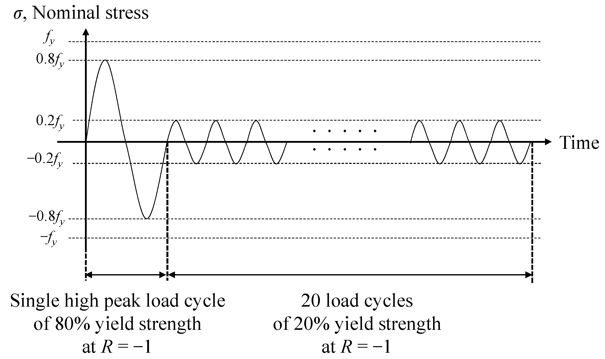
  • At the HFMI groove bottom, the in-depth profiles of residual stress showed the high compressive stress of about −0.30fy to −0.76fy within 0.5 mm of depth. The compressive stresses were maintained up to the depths in the range of 0.70 to 1.60 mm and were shifted to tensile stresses more deeply, which in-depth gradient was even steeper than that observed on available data of S355 steel grade. The high peak stress equal to 0.8fy led to a significant reduction of the beneficial compressive stresses, which, after relaxation, were close to zero near the surface and up to 1.2 mm, and remain tensile more deeply.
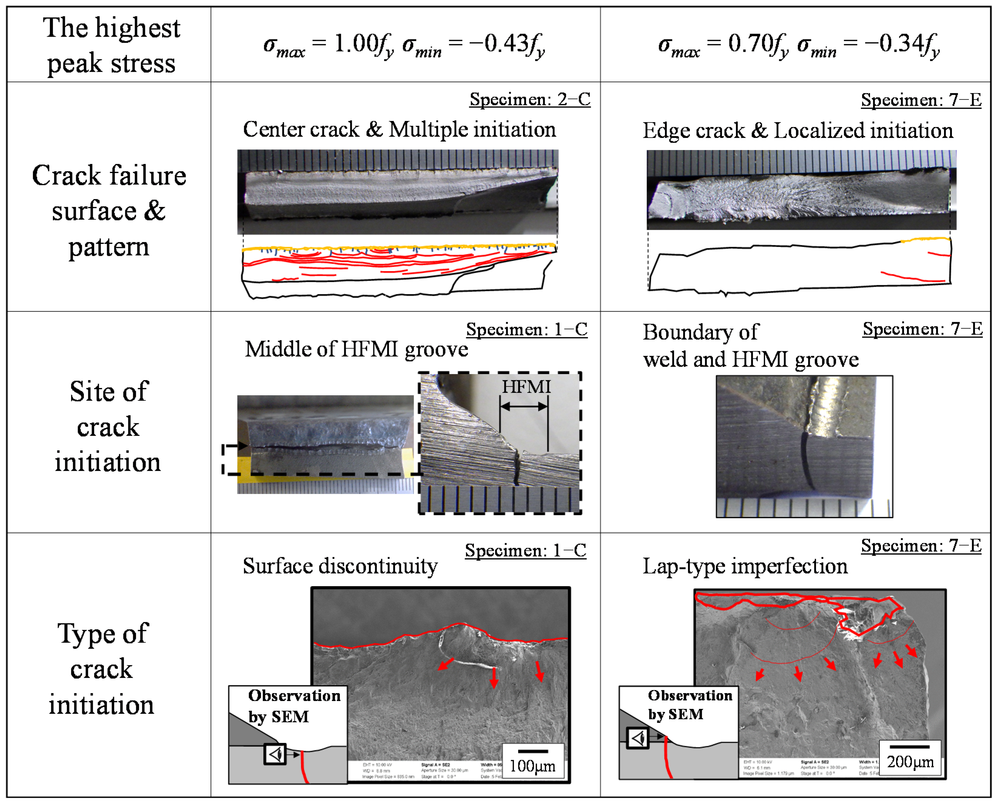
  • Different features on fracture surface, crack pattern, crack initiation site, and crack initiation type were observed according to different applied high peak stresses. Particularly interesting, as the applied peak stress was lowered from 1.0fy to 0.7fy, the initiation site within the weld shifted from the HFMI groove to near the boundary between the HFMI-treated zone and the weld metal. In the latter case, the lap-type imperfections for the site near the boundary became the origin of crack initiation.
For the numerical investigation:
  • The FE models developed, incorporating the measured in-depth residual stress profiles and applied load cycle with high peak load, was able to reproduce the residual stresses after relaxation; however, it was accurate only at the near surface with the HFMI treatment region.
  • The simulation results with the FE models demonstrated that the significant reduction of compressive residual stress near the surface, observed in residual stress measurement, was mainly occurred by compressive peak stress, as it led to immediate local yielding on the compressive sides of the HFMI treatment region.
For the fatigue damage assessment:
  • The damage-based assessment considering the local mean stress after high peak stress equal to 1.0fy and 0.7fy confirmed a shift of the crack initiation most prone position along the surface of the HFMI groove, resulting from a combination of stress concentration and relaxation effect of residual stresses.
  • When the peak stress was equal to 1.0fy, full relaxation of the compressive residual stress took place, such that cracks initiated from the HFMI groove where the stress concentration was dominant; less relaxation occurred under the peak stress equal to 0.7fy. Thus, in the latter case, the lap-type imperfections located near the boundary of the treatment became more critical for initiating the cracks even though the stress concentration was smaller than that of the HFMI groove. The above explains and confirms the experimental observations.

Author Contributions

Conceptualization, Y.O., H.C.Y., K.K. and A.N.; methodology, Y.O., H.C.Y. and A.N.; software, Y.O. and H.C.Y.; validation, Y.O.; formal analysis, Y.O.; investigation, Y.O., H.C.Y., K.K. and A.N.; resources, Y.O., H.C.Y. and A.N.; data curation, Y.O.; writing—original draft preparation, Y.O.; writing—review and editing, H.C.Y., K.K. and A.N.; visualization, Y.O.; supervision, H.C.Y., K.K. and A.N.; project administration, H.C.Y.; funding acquisition, Y.O., H.C.Y. and K.K. All authors have read and agreed to the published version of the manuscript.

Funding

This research was mainly conducted during study abroad of the first author at EPFL and Aarhus University, supported by two scholarships: scholarship in the Japan Public–Private Partnership Student Abroad Program (Tobitate! Young Ambassador Program) from the Japanese Student Services Organization (JASSO) and the Valor & V-drug Study Abroad Scholarship from Gifu University. A part of this research was funded by the European Project Hi-Life of Horizon 2020 with the Grant ID 702233, in which the second author is project manager.

Institutional Review Board Statement

Not applicable.

Informed Consent Statement

Not applicable.

Data Availability Statement

Not applicable.

Acknowledgments

The authors gratefully appreciated the valuable discussions and scientific input from Heikki Remes, from Aalto University. The authors would like to thank Sylvain Demierre from EPFL for his support in performing the fatigue tests and Gregoire Baroz from EPFL for SEM training, sample preparation, and micrograph imaging. Our special thanks go to ILL and Pirling Thilo, as well as Paul Lefevre from SONATS, for the residual stress measurements, and Salim Sleiman Nazzal from Aarhus University for sharing numerical modelling techniques.

Conflicts of Interest

The authors declare no conflict of interest.

Appendix A

Table A1. Detailed information of literature on specimen geometry and residual stress measurement method.
RefAuthorSteel Grade (fy)Specimen GeometryMethod of Residual Stress Measurement
L × W × TH × tgh
[31]Kuhlman. 2006S690QL (813 MPa)23 × 160 × 1218 × 125.7·Hole drilling (1.80 mm hole): 1.5 mm away from weld toe
[32]Kuhlman. 2009S690QL (830 MPa)26 × 80 × 1240 × 127.1·Hole drilling (1.77 mm hole): 1.0 mm away from weld toe
[35]Ranjan. 2016A514 (793 MPa)19 × 30 × 9.525 × 6.46.4·Laser X-ray diffaction (sin2ψ) & Layer removal by electronic poslihing
[27]Yildirim. 2020 & This studyS690QL (832 MPa)14 × 40 × 640 × 64.2·X-ray diffaction (sin2ψ, 1-mm collimator)
·Nutron diffraction at SALSA (0.6 × 2.0 × 0.6 mm3 or 2.0 × 2.0 × 2.0 mm3 collimator)
[33]Tehrani Yekta. 2012350W (396 MPa)19 × 30 × 9.525 × 6.46.4·Laser X-ray diffaction (sin2ψ) & Layer removal by electronic poslihing
[14]Quilliec. 2013S355K2 (490 MPa)-×-×15-×15-·X-ray diffraction (2.5 × 1.0 × 0.006 mm3 collimator)
[34]Suzuki. 2014SM490 (≥325 MPa)-×100 × 1650 × 16-·X-ray diffraction
·Neutron-diffraction (2.0 × 2.0 × 2.0 mm3 collimator)
[36]Leitner. 2015S355 (≥350 MPa)-×90 × 1340 × 16-·X-ray diffaction (sin2ψ, 1-mm collimator)
[37]Polezhayeva. 2015080A15 (560 MPa)46 × 80 × 2050 × 2013·Neutron-diffraction at UK’s ISIS neutron source (1-mm collimator )
[22]Schubnell. 2020S355J2 + N (420 MPa)21 × 50 × 1050 × 105.7·X-ray diffaction (2-mm collimator)
·Neutron diffraction (2.0 × 2.0 × 2.0 mm3 or 2.0 × 2.0 × 5.0 mm3 collimator)
L: toe-to-toe length (mm), W: main plate width (mm), T: main plate thickness (mm), H: gusset height (mm), tg: gusset thickness (mm), h: weld leg length (mm).
Table A2. Detailed information of literature on HFMI treatment condition.
RefAuthorMethodUltrasonic Frequency (kHz)Ultrasonic Amplitude (μm)Impact Frequency (Hz)Indenter Diameter, D or Tip Radius, R (mm)Travel Speed (m/mm)Note
[31]Kuhlman. 2006UIT27 3 (D) Power consumption: 900 W
[32]Kuhlman. 2009PIT 902.0(R)8.0(D)/2.5(R)8.0(D)2–3Working pressure: 6 bars
Angle for plate: 50–70 degree
[35]Ranjan. 2016UIT2050–602203.0(R)
[27]Yildirim. 2020 & This studyUNP2030–60100–4001.5(R) Angle for plate: 45 degree
Angle for travel direction: 90 degree
[33]Tehrani Yekta. 2012UIT 27–29 6.0Number of pass: 4
Angle for plate: 30–60 degree
Groove radius: 1.69–2.37
Groove depth: 0.27–0.36
[14]Quilliec. 2013UIT27 3.0(D)4.0Power consumption: 1200 W Number of pass: 1
Indenter: 3 pins
Angle for plate: 67 degree
[34]Suzuki. 2014UIT2730 3.0(R)6.0Power consumption: 1000 W
[36]Leitner. 2015PIT 2.0(R)0.6–1.8Angle for plate: 30–60 degree Angle for travel direction: 90 degree
[37]Polezhayeva. 2015UIT
[22]Schubnell. 2020PIT 90 Working pressure: 6 bars

References

  1. Statnikov, E.S. Application of Operational Ultrasonic Impact Treatment (UIT) Technologies in Production of Welded Joints; IIW Doc. XIII-1667-97; International Institute of Welding: Paris, France, 1997; Available online: http://www.appliedultrasonics.com/pdf/APPLICATIONS_OF_OPERATIONAL_ULTRASONIC_IMPACT_TREATMENT_(UIT)_TECHNOLOGIES_IN_PRODUCTION_OF_WELDED_JOINTS.html (accessed on 26 December 2021).
  2. Roy, S.; Fisher, J.W.; Yen, B.T. Fatigue resistance of welded details enhanced by ultrasonic impact treatment (UIT). Int. J. Fatigue 2003, 25, 1239–1247. [Google Scholar] [CrossRef]
  3. Huo, L.; Wang, D.; Zhang, Y. Investigation of the fatigue behaviour of the welded joints treated by TIG dressing and ultrasonic peening under variable-amplitude load. Int. J. Fatigue 2005, 27, 95–101. [Google Scholar] [CrossRef]
  4. Tominaga, T.; Matsuoka, K.; Sato, Y.; Suzuki, T. Fatigue improvement of weld repaired crane runway girder by ultrasonic impact treatment. Weld. World 2008, 52, 50–62. [Google Scholar] [CrossRef]
  5. Weich, I.; Ummenhofer, T.; Nitschke-Pagel, T.; Dilger, K.; Eslami, H. Fatigue behaviour of welded high-strength steels after high frequency mechanical post-weld treatments. Weld. World 2009, 53, 322–332. [Google Scholar] [CrossRef]
  6. Kudryavtsev, Y.; Kleiman, J. Increasing Fatigue Strength of Welded Joints by Ultrasonic Impact Treatment; IIW Document XIII- 2338-10; International Institute of Welding: Paris, France, 2010; Available online: http://sintes.ca/documents/IIWDocumentXIII-2338-10.2010UIT-UP.pdf (accessed on 26 December 2021).
  7. Maddox, S.J.; Dore, M.J.; Smith, S.D. A case study of the use of ultrasonic peening for upgrading a welded steel structure. Weld. World 2011, 55, 56–67. [Google Scholar] [CrossRef]
  8. Yıldırım, H.C.; Leitner, M.; Marquis, G.B.; Stoschka, M.; Barsoum, Z. Application studies for fatigue strength improvement of welded structures by high-frequency mechanical impact (HFMI) treatment. Eng. Struct. 2016, 106, 422–435. [Google Scholar] [CrossRef]
  9. Marquis, G.; Barsoum, Z. IIW Recommendation on High Frequency Mechanical Impact (HFMI) Treatment for Improving the Fatigue Strength of Welded Joints. In IIW Recommendations for the HFMI Treatment; Springer: Singapore, 2016; pp. 1–34. Available online: https://link.springer.com/chapter/10.1007/978-981-10-2504-4_1 (accessed on 26 December 2021).
  10. Yildirim, H.C. Recent results on fatigue strength improvement of high-strength steel welded joints. Int. J. Fatigue 2017, 101, 408–420. [Google Scholar] [CrossRef]
  11. Leitner, M.; Barsoum, Z. Effect of increased yield strength, R-ratio, and plate thickness on the fatigue resistance of high-frequency mechanical impact (HFMI)-treated steel joints. Weld. World 2020, 64, 1245–1259. [Google Scholar] [CrossRef]
  12. Mori, T.; Shimanuki, H.; Tanaka, M. Influence of steel static strength on fatigue strength of web-gusset welded joints with UIT. J. JSCE 2014, 70, 210–220. (In Japanese) [Google Scholar] [CrossRef]
  13. Lihavainen, V.M.; Marquis, G. Fatigue life estimation of ultrasonic impact treated welds using a local strain approach. Steel Res. Int. 2008, 77, 896–900. [Google Scholar] [CrossRef]
  14. Quilliec, L.G.; Lieurade, H.P.; Bousseau, M.; Drissi-Habti, M.; Inglebert, G.; Macquet, P.; Jubin, L. Mechanical and modelling of high-frequency mechanical impact and its effect on fatigue. Weld. World 2013, 57, 97–111. [Google Scholar] [CrossRef]
  15. Schubnell, J.; Hardenacke, V.; Farajian, M. Strain-based critical plane approach to predict the fatigue life of high frequency mechanical impact (HFMI)-treated welded joints depending on the material condition. Weld. World 2017, 61, 1199–1210. [Google Scholar] [CrossRef]
  16. Schubnell, J.; Pontner, P.; Wimpory, R.C.; Farajian, M.; Schulze, V. The influence of work hardening and residual stresses on the fatigue behavior of high frequency mechanical impact treated surface layers. Int. J. Fatigue 2020, 134, 105450. [Google Scholar] [CrossRef]
  17. Yıldırım, H.C.; Marquis, G.B. A round robin study of high frequency mechanical impact (HFMI)-treated welded joints subjected to variable amplitude loading. Weld. World 2013, 57, 437–447. [Google Scholar]
  18. Mikkola, E.; Doré, M.; Marquis, G.B.; Khurshid., M. Fatigue assessment of high-frequency mechanical impact (HFMI)-treated welded joints subjected to high mean stresses and spectrum loading. Fatigue Fract. Eng. Mater. Struct. 2015, 38, 1167–1180. [Google Scholar] [CrossRef]
  19. Leitner, M.; Stoschka, M.; Ottersböck, M. Fatigue assessment of welded and high frequency mechanical impact (HFMI) treated joints by master notch stress approach. Int. J. Fatigue 2017, 101, 232–243. [Google Scholar] [CrossRef]
  20. Leitner, M.; Stoschka, M.; Barsoum, Z.; Farajian, M. Validation of the fatigue strength assessment of HFMI-treated steel joints under variable amplitude loading. Weld. World 2020, 64, 1681–1689. [Google Scholar] [CrossRef]
  21. Tai, M.; Miki, C. Improvement effects of fatigue strength by burr grinding and hammer peening under variable amplitude loading. Weld. World 2012, 56, 109–117. [Google Scholar] [CrossRef]
  22. Schubnell, J.; Carl, E.; Farajian, M.; Gkatzogianis, P.; Knodel, P.; Ummenhofer, T.; Wimpory, R.; Eslami, H. Residual stress relaxation in HFMI-treated fillet welds after single overload peaks. Weld. World 2020, 64, 1107–1117. [Google Scholar] [CrossRef]
  23. Yonezawa, T.; Shimanuki, H.; Mori, T. Influence of cyclic loading on the relaxation behaviour of compressive residual stress induced by UIT. Weld. World 2020, 64, 171–178. [Google Scholar] [CrossRef]
  24. Mikkola, E.; Remes, H.; Marquis, G. A finite element study on residual stress stability and fatigue damage in high-frequency mechanical impact (HFMI)-treated welded joint. Int. J. Fatigue 2017, 94, 16–29. [Google Scholar] [CrossRef] [Green Version]
  25. Nazzal, S.S.; Mikkola, E.; Yıldırım, H.C. Fatigue damage of welded high-strength steel details impoved by post-weld treatment subjected to critical cyclic loading conditions. Eng. Struct. 2021, 237, 111928. [Google Scholar] [CrossRef]
  26. Ruiz, H.; Osawa, N.; Rashed, S. Study on the stability of compressive residual stress induced by high-frequency mechanical impact under cyclic loadings with spike loads. Weld. World 2020, 64, 1855–1865. [Google Scholar] [CrossRef]
  27. Yıldırım, H.C.; Remes, H.; Nussbaumer, A. Fatigue properties of as-welded and post-weld-treated high-strength steel joints: The influence of constant and variable amplitude loads. Int. J. Fatigue 2020, 138, 105687. [Google Scholar] [CrossRef]
  28. Mikkola, E.; Marquis, G.; Lehto, P.; Remes, H.; Hänninen, H. Material characterization of high-frequency mechanical impact (HFMI)-treated high-strength steel. Mater. Des. 2016, 89, 205–214. [Google Scholar] [CrossRef]
  29. SONATS. Residual Stress Measurement by X-ray Diffraction. Available online: https://sonats-et.com/en/residual-stress/x-ray-diffraction-services/ (accessed on 26 September 2021).
  30. Pirlinga, T. Precise analysis of near surface neutron strain imaging measurements. Procedia Eng. 2011, 10, 2147–2152. [Google Scholar] [CrossRef] [Green Version]
  31. Kuhlmann, U.; Durr, A.; Bergmann, J.; Thumser, R. Fatigue Strength Improvement for Welded High Strength Steel Connections Due to the Application of Post-Weld Treatment Methods; FOSTA, Forschung fur die Praxis P 620: Dusseldorf, German, 2006. (In Germany) [Google Scholar]
  32. Kuhlmann, U.; Gunther, H. Experimentelle Untersuchungen zur Ermüdungssteigernden Wirkung des PIT-Verfahrens; Universität Stuttgart Institut für Konstruktion und Entwurf: Stuttgart, Germany, 2009. (In Germany) [Google Scholar]
  33. Tehrani Yekta, R. Acceptance Criteria for Ultrasonic Impact Treatment of Highway Steel Bridges. Ph.D. Thesis, University of Waterloo, Waterloo, AB, Canada, 2012. [Google Scholar]
  34. Suzuki, T.; Okawa, T.; Shimanuki, H.; Nose, T.; Suzuki, H.; Moriai, A. Effect of ultrasonic impact treatment (UIT) on fatigue strength of welded joints. Adv. Mat. Res. 2014, 996, 736–742. [Google Scholar] [CrossRef] [Green Version]
  35. Ranjan, R.; Ghahremani, K.; Walbridge, S.; Ince, A. Testing and fracture mechanic analysis of strength effects on the fatigue behaviour of HFMI-treated welds. Weld. World 2016, 60, 987–999. [Google Scholar] [CrossRef]
  36. Leitner, M.; Mossler, W.; Putz, W.; Stoschka, M. Effect of post-weld heat treatment on the fatigue strength of HFMI-treated mild steel joints. Weld. World 2015, 59, 861–873. [Google Scholar] [CrossRef]
  37. Polezhayeva, H.; Howarth, D.; Kumar, M.; Ahmad, B.; Fitzpatrick, M.E. The Effect of compressive fatigue loads on fatigue strength of non-load carrying specimens subjected to ultrasonic impact treatment. Weld. World 2015, 59, 713–721. [Google Scholar] [CrossRef]
  38. Anami, K.; Miki, C.; Tani, H.; Yamamoto, H. Improving fatigue strength of welded joints by hammer peening and Tig-dressing. J. JSCE 2000, 17, 67–78. [Google Scholar] [CrossRef] [Green Version]
  39. Fisher, W.J.; Sullivan, M.D.; Pense, W.A. Improving Fatigue Strength and Repairing Fatigue Damage; Fritz Laboratory Reports, Paper 2067; Lehigh University: Bethlehem, PA, USA, 1974. [Google Scholar]
  40. Voce, E. The relationship between stress and strain for homogeneous deformation. J. Met. 1948, 74, 537–562. [Google Scholar]
  41. Garcia, M. Multiaxial Fatigue Analysis of High-Strength Steel Welded Joints Using Generalized Local Approaches. Ph.D. Thesis, EPFL, Lausanne, Switzerland, 2020. [Google Scholar]
  42. Smith, M. Abaqus/Standard User’s Manual, Version 6.9; Dassault Systèmes Simulia Corp.: Johnston, RI, USA, 2009. [Google Scholar]
  43. Smith., K.N.; Watson, P.; Topper, T.H. A stress-strain function for the fatigue of metals (stress-strain function for metal fatigue including mean stress effect). J. Mater. 1970, 5, 767–778. [Google Scholar]
  44. Kujawski, D. A deviation version of the SWT parameter. Int. J. Fatigue 2014, 67, 95–102. [Google Scholar] [CrossRef]
Figure 1. Configuration of the non-load-carrying attachments, Reprinted with permission from ref. [27]. 2021 International Journal of Fatigue (in axonometry and pictures showing weld geometries).
Metals 12 00145 g001
Figure 2. Applied load cycles at the constant amplitude of stress ratio R = −1.
Metals 12 00145 g002
Figure 3. Measurement points and paths through the thickness for XRD and ND methods.
Metals 12 00145 g003
Figure 4. Applied load sequence of the cumulative amplitude distribution, Reprinted with permission from ref. [27]. 2021 International Journal of Fatigue.
Metals 12 00145 g004
Figure 5. Residual stress profiles of AW, HFMI and HFMI-LC through thickness.
Metals 12 00145 g005
Figure 6. Comparison between measurement results and existing data for HFMI specimens and for two different steels at x = 0 mm.
Metals 12 00145 g006
Figure 7. Fatigue test results of S690QL in AW and HFMI conditions.
Metals 12 00145 g007
Figure 8. Observation results of fatigue crack initiation sites under different high peak stresses in the HFMI condition.
Metals 12 00145 g008
Figure 9. The global and local geometry for HFMI-treated detail.
Metals 12 00145 g009
Figure 10. Experiment-based in-depth residual stress distribution at x = 0 mm.
Metals 12 00145 g010
Figure 11. Implemented residual stress distribution in FE model.
Metals 12 00145 g011
Figure 12. Numerical and experimental comparison of the residual stress distributions after the stress relaxation at x = 0 mm. (a) HC case as FE input; (b) LC case as FE input.
Metals 12 00145 g012
Figure 13. Change of residual stress state due to the applied load cycles in the FE model.
Metals 12 00145 g013
Figure 14. Applied load cycles for fatigue damage assessment.
Metals 12 00145 g014
Figure 15. Positions subjected to SWT damage parameter.
Metals 12 00145 g015
Figure 16. Comparison of fatigue damage distribution along the HFMI-treated surface between different high peak stresses.
Metals 12 00145 g016
Table 1. Mechanical properties and chemical compositions of S690QL.
SteelMechanical PropertiesChemical Composition
Yield Strength fy (N/mm2)Tensile Strength fu (N/mm2)Elongation (%), MinimumCSiMnPSAlNbVTiCuCrNiMoCaNEW
S690QL83285600.140.291.210.0110.0010.0470.0210.0280.100.0100.280.050.1500.00.0020.43
Table 2. Test matrix of residual stress measurements.
Condition NameXRDNDNote
Meas. Points 0 mmMeas. PathsMeas. PathsMeas. Paths
TopBottomTopBottomTopBottom
AW-111111Initial state
HFMI4111111Initial state
HFMI-LC--1-1-1After load cycles in Figure 2
Table 3. Fatigue test results and fracture observation of S690QL in HFMI condition.
Specimen NumberThe Highest Peak Stress in a Part of Variable Amplitude LoadingThe Number of Cycles to Complete Failure, NCrack Location
Δσmaxσmaxσmin
1−C1191 MPa1.00fy (833 MPa)−0.43fy (358 MPa)258750Center
2−C1191 MPa1.00fy (833 MPa)−0.43fy (358 MPa)346500Center
3−C1191 MPa1.00fy (833 MPa)−0.43fy (358 MPa)492000Center
4−E911 MPa0.80fy (665 MPa)−0.37fy (246 MPa)2565750Edge
5−E911 MPa0.80fy (665 MPa)−0.37fy (246 MPa)2637000Edge
6−C911 MPa0.80fy (665 MPa)−0.37fy (246 MPa)4788750Center
7−E780 MPa0.70fy (582 MPa)−0.34fy (198 MPa)2499000Edge
8−E780 MPa0.70fy (582 MPa)−0.34fy (198 MPa)5466000Edge
9−E780 MPa0.70fy (582 MPa)−0.34fy (198 MPa)6579000Edge
Table 4. Voce-Chaboche’s (VC) parameters for high-strength steels of S690 grade presented by Garcia, data from ref. [41].
NameAuthorMaterialLinear-Elastic BehaviorNon-Linear Behavior
Elastic PropertiesIsotropic PropertiesKinematic Properties
E [MPa]νQqσy [MPa]C1γ1C2γ2
BM-1GarciaBase material2100000.300578183281742188
BM-2Castro e SousaBase material2060000.30159019018837715
BM-3MikkolaBase material2000000.3117721147839511478395
E: Young modulus, ν: Poisson ratio, Q: Maximum increase in size of yield surface due to hardening at saturation, q: How quickly the increase of yield surface approaches the saturation, σy: Yield stress at zero plastic strain, C: Initial kinematic hardening modulus, γ: Rate at which the kinematic hardening modulus decreases with increasing plastic deformation.
Publisher’s Note: MDPI stays neutral with regard to jurisdictional claims in published maps and institutional affiliations.

