Article

Development of Data-Driven Machine Learning Models for the Prediction of Casting Surface Defects

1
Mathematics for Engineers, Institute for Technologies of Metals, University of Duisburg-Essen, Friedrich-Ebert-Str. 12, 47119 Duisburg, Germany
2
Manufacturing Technology-Foundry Technology, University of Applied Sciences Kempten, Bahnhofstraße 61, 87435 Kempten, Germany
*
Authors to whom correspondence should be addressed.
These authors contributed equally to this work.
Metals 2022, 12(1), 1; https://doi.org/10.3390/met12010001
Submission received: 2 November 2021 / Revised: 10 December 2021 / Accepted: 17 December 2021 / Published: 21 December 2021
(This article belongs to the Special Issue Optimizing Techniques and Understanding in Casting Processes)

Abstract

:
This paper presents an approach for the application of machine learning in the prediction and understanding of casting surface related defects. The manner by which production data from a steel and cast iron foundry can be used to create models for predicting casting surface related defect is demonstrated. The data used for the model creation were collected from a medium-sized steel and cast iron foundry in which components ranging from 1 to 100 kg in weight are produced from wear and heat resistant cast iron and steel materials. This includes all production-relevant data from the melting and casting process, as well as from the mold production, the sand preparation and component quality related data from the quality management department. The data are tethered together with each other, the information regarding the identity and number of components that resulted in scrap due to the casting surface defect metal penetrations was added to the dataset. Six different machine learning algorithms were trained and an interpretation of the models outputs was accomplished with the application of the SHAP framework.

Graphical Abstract

1. Introduction

In the coming years, the foundry industry will have to face ever greater challenges in terms of resource and energy optimization due to the expected ecological and economic change towards a climate-neutral Europe. In order to curb climate change and prevent a further increase in the earth’s temperature, the European Union has launched the “European Green Deal” in 2019. This political and economical program aims to extend the current target of reducing the European Union’s CO 2 emissions by 40 percent (by 2030 compared to 1990 levels) to a reduction of 50 to 55 percent [1]. For this reason, sustainability and resource conservation are moving to the center of the future business orientation of the manufacturing industry, especially the foundry industries. The foundry industry, which is one of the most energy-intensive industries in Germany, employs 70,000 people in around 600 iron, steel, and non-ferrous metal foundries. The economic importance of this sector, which is mostly structured as medium-sized enterprises, results from its classic supplier function and its role as a key sector for the automotive and mechanical engineering industries. From this leading position, foundries have to face a variety of technological, economic, and sustainability-related challenges, as well as increasing competitive pressure: Competition from emerging markets, increased demands for flexibility, rising delivery, and quality pressure, the strategic goal of a CO 2 -neutral Europe, and increasing globalization are forcing new approaches to maintain competitiveness. Against this backdrop, sustainable safeguarding of future viability requires the consistent further development of process technology and control through the application of intelligent, adaptive manufacturing techniques. There is a big potential in the digitization of the process chain to make manufacturing more resilient, sustainable and flexible. The continuing dynamic development of digitization and the associated methods and technologies have a considerable influence on the requirements and designs of production systems. For efficient use of production data, data analysis with machine learning methods or by means of deep learning and transfer learning approaches and a reflection of the analysis results back into production is essential, whereby so-called cyber-physical production systems can be built [2]. By using cyber-physical production systems, the optimization of individual processes or parameters, as well as the optimization of the process chain is possible [3]. Thus, a sustainable process design is achievable in order to meet increasingly complex process requirements. Various approaches for the application of AI methods and assistance apps in the foundry industry already exist, such as [4,5,6,7,8]. However, a holistic ecosystem of assistance application for the complete foundry production system does not exist. One possible factor achieving the above-mentioned goals of resource and energy optimization is the reduction of scrap rates. High scrap rates weigh doubly detrimental to the resource and energy balance, as components that have already been cast are required to be melted down and manufactured again. This case study, therefore, investigates to what extent machine learning can help model the problem of casting surface defects (exemplary metal penetration) in a foundry and draw conclusions for the manufacturing process.

Casting Surface Defects

In the steel and cast iron industry, where the production of components is carried out using sand molds, it is well known that the biggest reason for components resulting in scrap post production is often times the mold material and its quality properties. Insufficient mold and core quality can be the reason for up to 40–50% of the overall scrap rate in a foundry. One of these casting surface defects is the metal penetration. The defect leads, if not directly to scrap, then to a considerable increase in finishing work post-production, and therefore to additional manufacturing costs. Metal penetration is a highly complex casting defect and there are many reasons why it can occur, to only name a few: overly large grain size and wide grain distribution in the mold material, insufficient binder content, insufficient proportion of lustrous carbon forming substances and gas permeability in the mold, excessive compactability of the mold and unfavorable chemical composition of the melt in connection with exceedingly high casting temperature and high metallostatic pressure, as well as insufficient and or uneven compression of the molds or cores. Melting phases form as a result of metal-mold reactions, resulting in scorched sand (sintering) and mineralization. When casting alloyed steel, this fault is quite common. On the casted component, it is evident to the naked eye. Edges in the sand mold or sand core, where the metal remains liquid for a long period due to the geometry of the casting and the molded pieces severely heated, are preferred mineralization areas. Mineralization, unlike real mechanical/physical penetration, is a chemically generated penetration. Burnt sand is still referred to when a thin sand crust of individual quartz grains adheres strongly to the casting (sintering). Mineralization occurs when this thin and now an extremely firmly adherent layer is made up of fused sand, giving the entire surface a pockmarked look [9]. As seen from above there are multiple reasons for these defects to occur, many of them are connected with each other due to multi-parametric relationships and therefore difficult to analyze.

2. Machine Learning

Machine Learning (ML) is regarded as programming computers to optimize a capability criterion using sample data or experience [10]. Machine Learning concentrates on the development of computer programs that can access data and employ it to learn for themselves automatically. For the past few years, machine learning has received much attention. Due to the growing volumes and varieties of available data, computational processing that is cheaper and more powerful, all of this trends enable a more complex, robust, and accurate system to be built, which are capable of any of the facilities that are associate with intelligence, such as computer vision, natural language processing, automotive, manufacturing, foundry, etc.
In practice, machine learning algorithms can be divided into three main categories based on their purpose. Supervised learning occurs when an ML model learns from sample data and associated target responses that can consist of numeric values or string labels, such as classes or tags, to later predict the correct response when posed with new examples Ref. [11]. Supervised learning is frequently applied in applications where historical data predicts likely future events. Generally, supervised learning problems are categorized into classification and regression. In regression problems, the model tries to predict results within a continuous output based on the continuous functions. For example, it can predict the price of a house according to the size and the living area. In contrast to regression, in classification output is predicted in discrete value, such as yes or no, true or false, positive or negative, etc. For instance, given an image, correctly classify whether the content is composed of cats or dogs (or a combination of the both).
Unlike supervised learning, which is trained using labeled examples, an unsupervised learning model is prepared by deducing structures present in the input data without any associated response, leaving the algorithm to determine the data patterns on its own [11]. A typical example is the recommendation system, it can determine segments of customers with similar characteristics who can then be treated similarly in marketing campaigns. There are many popular techniques including clustering and dimension reduction. Reinforcement learning is concerned with the issue of how to interact with the environment and to choose suitable actions in a given situation, to maximize the reward [12]. This type of learning is often used for robotics, gaming, and navigation since these applications must make decisions and the decisions bear consequences.
In this case the prediction of the casting quality of steel components produced by the sand casting process, algorithms for this purpose are supervised learning, in addition to the algorithms from the category regression. The basic workflow of a machine learning project are given below.

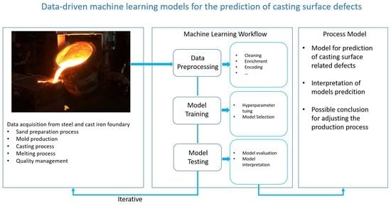
2.1. Machine Learning Workflow

Machine Learning workflows define the phases initiated during a particular machine learning implementation. We can define the machine learning workflow in 4 steps, which shows in Figure 1:
  • Data acquisition;
  • Data pre-processing;
  • Training the model;
  • Model evaluation.

2.1.1. Data Acquisition

To start a machine learning project, the first step is to collect data from relevant sources. It is the process of retrieving relevant manufacturing information, transforming the data into the required form, and loading it into the designated system. The dataset collected from the foundry industry comes from different sources, such as ERP databases, IoT devices, and so on.

2.1.2. Data Pre-Processing

Once the data are collected, it needs to be pre-processed. Pre-processing involves cleaning, verifying, and formatting data into a usable dataset. It is the most important step that helps in building machine learning models more accurately. The very first step of pre-processing is to identify missing data. Missing data are common in most real-world datasets. These missing values need to first be handled to optimally leverage available data. A fundamental strategy when using incomplete datasets is to discard entire rows or columns containing missing values. However, this comes at the price of losing informative data which may be valuable for model training. By contrast, imputation tries to infer the missing values from the known part of the data. Some well-known methods include replacing missing values with zero, mean, median, or mode.
In general, learning algorithms benefit from standardization of the dataset. Different columns can be present in varying ranges. For example, there can be a column with a unit of distance, and another with the unit of temperature. Those columns will have strongly different ranges, making it difficult for many machine learning models to reach an optimal computational state. There are some techniques to address this problem, they are standardization, or mean removal and variance scaling; scaling features to a range, often between zero and one, or so that the maximum absolute value of each feature is scaled to unit size.
In many cases, data are in a format that cannot be processed by algorithms. For instance, a column with string values or text, will mean nothing to a model that only accepts numerical values as input. So it is necessary to convert the categorical features to integer codes to help the model interpret it. This method is called categorical encoding. Some popular methods include ordinal encoding, which embeds values from 1 to n in an ordinal manner, n is the number of samples in the column. If a column has 3 city names, ordinal encoding will assign values 1, 2, and 3 to the different cities. One hot encoding can be used when data has no inherent order. One hot encoding generates one column for every category and assigns a positive value 1 in whichever row that category is present, and 0 when it is a absent.
New features can be created from raw features, this is called feature engineering. For example, the day, month, and year can be extracted from a date time column. This gives a new perspective to the model, which can now detect a brand new relation between time and the target variable. In a similar way, discretization is the process to partition continuous features into discrete values. Certain datasets with continuous features may benefit from discretization, because it can transform the data set of continuous attributes to one with only nominal attributes. Adding complexity to the model by considering non-linear features of the input data could be useful. A intuitive and common way is to use polynomial features, which can obtain features’ high-order and interaction terms. For instance, the features of X can be transformed form ( X 1 , X 2 ) to ( 1 , X 1 , X 2 , X 1 2 , X 1 X 2 , X 2 2 ) .

2.1.3. Training the Model

Before training the model, usually data need to be divided into two parts, training and testing:
  • Training set: used to initially train the algorithm and teach it how to process information;
  • Testing set: used to access the accuracy and performance of the model.
Once the dataset is ready to train, the next step involves feeding the training set to the algorithm so that it can learn appropriate parameters and features used in the learning process. The machine learning models applied in this research will be explained in Section 2.2.
To measure the model performance for regression problem, the following metrics are introduced:
  • Mean absolute error (MAE): is a loss metric corresponding to the expected value of the absolute error loss. If y ^ i is the predicted value of the i-th sample, and y i is the corresponding true value, n is the number of samples, the MAE estimated over n is defined as:
    MAE ( y , y ^ ) = 1 n i = 0 n 1 y i y ^ i
  • Mean squared error (MSE): is a loss metric corresponding to the expected value of the squared error. MSE estimated over n is defined as:
    MSE ( y , y ^ ) = 1 n i = 0 n 1 ( y i y ^ i ) 2
  • Root mean square error (RMSE): is the square root of value obtained from MSE:
    RMSE ( y , y ^ ) = M S E
  • R 2 score: represents the proportion of variance of y that has been explained by the independent variables in the model. It provides an indication of fitting goodness and, therefore, a measure of how well unseen samples are likely to be predicted by the model:
    R 2 ( y , y ^ ) = 1 i = 1 n ( y i y ^ i ) 2 i = 1 n ( y i y ¯ ) 2
  • Root mean squared logarithmic error (RMSLE): computes a risk metric corresponding to the expected value of the root squared logarithmic error:
    RMSLE ( y , y ^ ) = 1 n i = 0 n 1 ( log e ( 1 + y i ) log e ( 1 + y ^ i ) ) 2
Generally, many hyperparameters settings are involved in training machine learning models. A hyperparameter for a learning algorithm is defined as a variable to be set prior to the actual application of the algorithm to the data, one that is not directly learned from the training process [13]. Hyperparameters are tuned by running a whole training job, looking at the aggregate accuracy and adjusting. The most common search algorithms include grid search, random search and Bayesian optimization.

2.1.4. Model Evaluation

Finally, after an acceptable set of hyperparameters is found and model performance is optimized we can test the model. Testing uses the test dataset and is meant to verify that models are using accurate features. Based on the feedback received one may return to training the model to improve performance, adjust output settings, or deploy the model as needed.

2.2. Machine Learning Algorithm

2.2.1. Ridge Regression

Ridge regression is linear least squares with L 2 regularization. It addresses some of the problem of Ordinary Least Squares by imposing a penalty on the size of the coefficients. The ridge coefficients minimize a penalized residual sum of squares:
min w | | X w y | | 2 2 + α | | w | | 2 2
where X is input data, w = ( w 1 , , w p ) is coefficients vector for a linear model, y denotes the target value, and α 0 is the complexity parameter which controls the amount of shrinkage.

2.2.2. Random Forest Regression

A random forest algorithm [14] consists of many decision trees [15]. The random forest establishes the outcome based on the predictions of the decision trees. The forest generated by the random forest algorithm is trained through bagging [16] or bootstrap aggregating [17]. Bagging involves using different samples of data rather than just one sample, it utilizes a method to reduce the variance of a base estimator, by introducing randomization into its construction procedure and then making an ensemble out of it. On the other hand, bootstrap trains a sequence of weaker learners on repeatedly modified versions of data. The predictions from all of them are then combined through a weighted majority vote to produce the final prediction. A random forest eradicates the limitations of a decision tree algorithm. It reduces the overfitting of datasets and increases precision. It predicts by taking the average or mean of the output from various trees. Figure 2 shows the structure of a random forest.

2.2.3. Extremely Randomized Trees Regression

Compare to the random forest, extremely randomized trees (ET) [18] brings randomness one step further in the way splits are computed. ET do not resample observations when building a tree, instead, ET makes a small number of randomly chosen splits-points for each of the selected predictors, and selects the “best split” from this small number of choices. ET allows to reducing the variance of the model a bit more, at the expense of a slightly greater increase in bias.

2.2.4. XGBoost

XGBoost is short for “Extreme Gradient Boosting” [19], it is also a tree-based ensemble method like random forest. In addition to that, XGBoost incorporates another popular method called boosting [17], where successive trees add extra weight to samples which have been incorrectly predicted by earlier trees. This way the final predictions are obtained by a weighted vote of all trees [19]. It is called gradient boosting because it uses a gradient descent algorithm to minimize the loss when adding new models. By combining the strengths of these two algorithms, XGBoost has an excellent capacity for solving supervised learning problems.

2.2.5. CatBoost

CatBoost [20] is another ensemble algorithm that leverages from boosting, however, it works well with multiple categories of data. Compared to XGBoost, CatBoost also handles missing numeric values. CatBoost distinguishes with symmetric trees which use the same split in the nodes of each level, making it much faster than XGBoost. CatBoost calculates the residuals for each data point and does this with the model trained with other data. In this way, different residual data are obtained for each data point. These data are evaluated as targets and the general model is trained to the number of iterations.

2.2.6. Gradient Boosting Regression

The gradient boosting (GB) algorithm is used to generate an ensemble model by combining the weak learners or weak predictive models. It builds an additive model by using multiple decision trees of fixed size as weak learners. The process of fitting a GB model starts with the constant such as mean value of the target values. In subsequent stages, the decision trees or the estimators are fitted to predict the negative gradients of the samples. The gradients are updated in the each iteration.

2.3. Model Interpretation

The rapidly increasing usage of ML raises the attention of explainable ML to help people better trust and understand model at scale. Humans must be able to fully understand how decisions are being made so that they can trust the decision of an ML system. In principle, ML models are needed to function as expected, to produce transparent explanations, and to be visible in how they work.
Explainability is important in many ways. These include: ensuring fairness, looking for issues with bias in training data, regulatory, legal, and branding concerns, and simply studying the internals of a model to optimize it, to produce the best result. There are some criteria that can be used for categorizing model interpretation methods. For example, interpretability methods can be grouped based on whether they are intrinsic or post-hoc. They could also be model-specific or model agnostic. They can also be grouped according to whether they are local or global.
Recently, many methods have been developed to interpret prediction from supervised ML models. LIME [21] is an approach that can explain the predictions of any classifiers by learning an interpretable model locally around the prediction. DeepLIFT [22] is an example of a model-specific method for explaining deep learning models in which the contributions of all neurons in the network are back-propagated to the input features [23]. However, the Shapley Additive Explanation (SHAP) [24], which inspired these and several other methods [25,26,27,28], has often been proposed as a unit approach to explain the output of any ML model.
The Shapley value (SHAP) was originally proposed to estimate the importance of an individual player in a collaborative team [24,29]. SHAP interprets the Shapley value as an additive feature attribution method, and SHAP interprets the predicted value of the model as the sum of the attribution value of each input feature:
g ( z ) = ϕ 0 + j = 1 M ϕ j z j
where g is interpretation model, z { 0 , 1 } M indicates whether the corresponding feature can be observed (1 or 0). M is the number of input, and ϕ i R is the attribution value (Shapley value) of each feature. ϕ 0 is the constant of the interpretation model (namely the predicted mean value of all training samples) [24].
Lundberg and Lee [24] demonstrate that SHAP is better aligned with human intuition than other ML interpretation methods. There are three benefits worth mentioning here.
  • The first one is global interpretability—the collective SHAP framework can show how much each predictor contributes, either positively or negatively, to the target variable. The features with positive sign contribute to the final prediction activity, whereas features with negative sign contribute to the prediction inactivity. In particular, the importance of a feature i is defined by the SHAP as follow:
    ϕ i = 1 | N | ! S N \ { i } | S | ! ( | N | | S | 1 ) ! [ f ( S { i } ) f ( S ) ]
    Here, f ( S ) is the output of the ML model to be interpreted using a set of S of features, and N is the complete set of all features. The contribution of feature i ( ϕ i ) is determined as the average of its contribution among all possible permutations of a feature set. Furthermore, this equation considers the order of feature, which influence the observed changes in a model’s output in the presence of correlated features [30].
  • The second benefit is local interpretability—each observation obtains its own set of SHAP framework. This greatly increases its transparency. We can explain why a case receives its prediction and the contributions of the predictors. Traditional variable importance algorithms only show the results across the entire population but not for each individual case. The local interpretability enables us to pinpoint and contrast the impact of the factors.
  • Third, SHAP framework suggests a model-agnostic approximation for SHAP framework, which can be calculated for any ML model, while other methods use linear regression or logistic regression models as the surrogate models.
The core idea behind Shapley value based explanation of machine learning models is to use fair allocation results from cooperative game theory to allocate credit for model’s output f ( x ) among its input features. Furthermore, SHAP framework of all the input features will always sum up to the difference between baseline model output and the current model output for the prediction being explained, which means we can explicitly check the contribution of every feature on the individual label.

3. Experiments and Results

3.1. Introduction to Dataset

The production data used for the model development origins from a medium-sized steel and cast iron foundry in which components are cast from wear and heat resistant cast iron and steel materials. The range of materials includes many different grades such as 1.4848, 2.4879, 3.3243, or 3.5102. The metal is melted in a medium-frequency induction furnace (with a capacity of approximately 1t) and poured into bentonite-bonded sand molds. The dataset includes all production-relevant data from the melting and casting process (e.g., chemical composition of the melt measured with optical emission spectrometry, melting duration, casting temperature, holding time, etc.), as well as data from the quality management, such as sand related data (gas permeability, compactability, water content, etc.) and information about which and how many components of a 1t batch resulted in scrap or considerably increased need for finishing work due to metal penetrations. Quality control is carried out by testing the chemical composition of the melt with optical emission spectroscopy, mold sand testing is measured in the in-house sand lab by measuring the water and sediment content, mesh analyses/grain size distribution, compressive strength, wet tensile strength, compaction, and bulk weight. Table 1 shows an abstract of the used input variables. The amount of scrap of a certain batch of produced components is chosen as the target variable for the models. The components that are produced and are part of the used dataset range from very small components (for wear parts applications in blasting systems with a weight of approximately 1 kg) to bigger components (such as grids with a weight up to 70 kg). The original data collected in the foundry has 1079 rows and 52 columns (the different production process parameters that were mentioned above), around 1079 individual melt samples, 51 independent variables and one output variable and the amount of scrap for each batch in kg. The dataset was split into the training and testing datasets and account for 80% and 20% of the data, respectively. Figure 3 shows the concept of the machine learning approach.

3.2. Experiments Settings

To obtain optimal training results, some methods are addressed to pre-process the input data. First, the numerical missing values are imputed with median value of that specific column, and categorical missing values are replaced with the constant value. Second, all the numerical columns are scaled to unit norm, which reduce the impact of magnitude in the variance. Third, transformation is applied to some columns such that data can be represented by a normal or approximate normal distribution. Fourth, three columns which have too many unique values or few extreme values outside the expected range are discretized into categorical values using a pre-defined number of bins. Fifth, feature columns in the dataset that are highly linearly correlated with other feature columns will be dropped. Finally, to extend the scope of independent variables, new polynomial features that might help in capturing hidden relationships are created. After pre-processing the raw input data, the number of independent variables is increased from 51 to 282.

3.3. Experiments Results

The six above described machine learning algorithms were trained and tested. To find optimal hyperparameters of each algorithms, the Bayesian optimization was applied for minimizing objective functions. To find the best combinations of hyperparameters and decrease training error, a solution called cross-validation was employed. A testing set should still be held out for final evaluation. In the basic approach, the training dataset was divided in k groups, called f o l d s , of equal sizes. The prediction function is learned using k 1 folds, and the resulting model is validated on the remaining part of the data. In this setting, k is equal to 10. The performance measure reported by k f o l d cross-validation is then the average of the values computed in the loop. Table 2 provides the results of every machine learning algorithm on the training set.
After the hyperparameter tuning of every ML model, some relative important hyperparameters are shown on the Table 3. These hyperparameters will then be applied to every ML model to make predictions.
The ML models are evaluated on the training set using fore-mentioned scoring metrics. The ET algorithm has the best performance on the all five metrics comparing to other five models. After training the model, a model with the best hyperparameters of every ML model can be used to predict the final output on the testing dataset. Table 4 shows the metrics on the testing set of six models.
The result on the testing set is very similar to the training set, the ET algorithm outperforms the other five models in terms of all scoring metrics, it can be concluded that the ET has given the best response and an excellent result in the testing phase. So the ET algorithm will be chosen as the model for model interpretation and predictions.
Figure 4 demonstrates a residuals plot for the ET model. It shows the difference between the observed value of the target variable (y) and the predicted value ( y ^ ).

3.4. Global Model Interpretation Using SHAP

Global model interpretation means understanding the distribution of the prediction output based on the features, answering the question “how does the trained model make predictions”. The SHAP framework provides two ways to visualize global interpretation, feature importance and summary plot.
The idea behind SHAP feature importance is simple: features with large absolute Shapley values are important. After calculating the absolute Shapley values per feature across the data, the features will be sorted by decreasing importance. After pre-processing, the training dataset contains 282 features. The contribution of each individual feature is horizontally stacked and summed up. In general, it indicates that para_1 is the most important feature followed by attribute para_2 and para_3. These three features have greater mean SHAP framework than others. Changing the value of para_1 can cause the alteration of predicted output on average by 4.26. On the other hand, the very last 271 features contribute only insignificantly to the final prediction (sum of the top three parameters is higher than the sum of the combined 271 features), compared to the top 3 features. The result is shown in Figure 5.
The feature importance plot is useful, but contains no information beyond the importance. For a more informative plot, the summary plot (Figure 6) provides feature importance with feature effects. Each point on the summary plot is a Shapley value for a feature and an instance. The position on the y-axis is determined by the feature and on the x-axis by the Shapley value. The color represents the value of the feature from low to high. Overlapping points are jittered in the y-axis direction, the features are ordered according to their importance. From Figure 6 we can tell that a high level of the attribute para_1 (excessive content of organic binders in the mold material) and para_2 (exceedingly high fine particles content in the mold material) content have an impact on the final prediction. The high comes from red color, and positive is shown on the x-axis. Similarly, it can be assumed that the attribute para_3 is negatively correlated with the target variable.

4. Discussion and Conclusions

In this paper, it was shown how production data from the foundry environment can be used to develop data-driven prediction models for casting surface defects. To provide a basis of comparison, 6 ML regression methods were evaluated. Their hyperparameters were tuned carefully. Before training and testing, the dataset was first processed. On the used test data, the ET showed the best prediction results for the expected amount of rejected components ( R 2 = 0.75 , R M S E = 17 kg). The interpretation of the models using the SHAP framework provides a conclusive statement about the reasons for the casting defect metal penetration. Based on the SHAP framework, the prediction model indicates that the process variables para_1 (excessive content of organic binders in the mold material), para_2 (too high fines content in the mold material), and para_3 (insufficient gas permeability of the mold material), which all are related to measured mold quality, are some of the main influencing variables for the casting surface defect to occur. This is in line with information from the literature [9] and, additionally, the everyday experience of foundry engineers. In this respect, it can be seen that machine learning can provide a reasonable modeling of the production process. In this case the fact that these mold related parameters are critical and play a major role in these casting defects are well known, but the fact that the model is correctly identifying these critical chemical and physical parameters from the dataset shows the potential of the application of machine learning in the foundry environment. However one major problem is the consistency of the used data. From evaluation of the R2-value, it is clear that there must be more influencing parameters on the casting surface defects, that were not investigated, most likely due to the fact that they are not measured or well recorded and, therefore, not included in the given dataset. The biggest problem is most likely the quality of the data, for example, sand quality related data are only measured from certain sand samples taken out of the production process. At the moment it is not possible to have a conclusive in-line quality measurement of the used sand, therefore only the samples that were tested in the lab could have been evaluated. Overall it can be said that a more comprehensive model could be developed by implementing more process data, especially more accurate data from the sand quality testing, into the modeling.

Conclusions

In the foundry industry often times the reasons for bad quality production results are not well known, understood and or appear seemingly random. Machine learning could help with this as it is a conclusive and powerful tool to analyse big and complex data. The foundry environment with its data from the multiple sub-processes such as melting, sand preparation, and mold production, fits very well into the definition of complex data. However, for a practical use in the daily production environment and even some kind of automated control loop that helps adjusting the manufacturing process many challenges and problems in the foundry environment need to be resolved. One challenge for the effective use of machine learning in this environment is the lack of data collection and access. The foundry industry is characterized by a strong mixture of new and existing plants in a factory environment that has often grown historically. In these heterogeneous brownfield environments, complete digitization of production is associated with challenges, such as analog communication paths, lack of connectivity, media disruptions, and a large number of different machine controls [31]. This results in the following pain points for the foundry industry: data acquisition is often still performed manually even in key processes; fully automated, cross-system data acquisition exists only in the rarest cases; media discontinuities exist between existing systems and manual information acquisition; data quality is often highly heterogeneous and not sufficiently good for data-driven optimization; effective data utilization of process data often does not take place or only to a limited extent; process optimization is based on assumptions and experience, trial-and-error and, therefore, multi-parametric relationships are not or only very challengingly recognizable. This leads to high scrap rates, often times low process stability and, therefore, poor resource and energy efficiency. In the future, foundries will need very flexible, resilient, and efficient production. The pain points described above give rise to the overriding problem that a large number of efficiency potentials are currently not being exploited. On the one hand, these are of an economic nature, since production costs can be reduced, for example, through process optimization and a reduction in the scrap rate. On the other hand, there is considerable potential in the area of ecological sustainability, which can be leveraged, for example, through process optimization for reduced energy consumption, but also through targeted energy-optimized plant layout. In order to exploit these efficiency potentials and as described above to meet the increasing requirements, the complete digitization of production and use of machine learning seems the next step in optimizing production processes.

Author Contributions

Conceptualization, Data Collection, Methods implementation, and Writing: S.C. and T.K. All authors have read and agreed to the published version of the manuscript.

Funding

This research received no external funding.

Institutional Review Board Statement

Not applicable.

Informed Consent Statement

Not applicable.

Data Availability Statement

The data used for this article can be made available upon request through the corresponding author.

Conflicts of Interest

The authors declare no conflict of interest.

References

  1. Kommission, E. Mitteilung der Kommission an das Europäische Parlament, den Europäischen Rat, den Rat, den Europäischen wirtschafts- und Sozialausschuss und den Ausschuss der Regionen: Der Europäische Grüne Deal 2019. Available online: https://eur-lex.europa.eu/legal-content/DE/TXT/?uri/ (accessed on 1 October 2021).
  2. Thiede, S.; Juraschek, M.; Herrmann, C. Implementing cyber-physical production systems in learning factories. Procedia Cirp 2016, 54, 7–12. [Google Scholar] [CrossRef] [Green Version]
  3. Lee, J.; Noh, S.D.; Kim, H.J.; Kang, Y.S. Implementation of cyber-physical production systems for quality prediction and operation control in metal casting. Sensors 2018, 18, 1428. [Google Scholar] [CrossRef] [PubMed] [Green Version]
  4. Ferguson, M.; Ak, R.; Lee, Y.T.T.; Law, K.H. Automatic localization of casting defects with convolutional neural networks. In Proceedings of the 2017 IEEE International Conference on Big Data (Big Data), Boston, MA, USA, 11–14 December 2017; pp. 1726–1735. [Google Scholar]
  5. Fernández, J.M.M.; Cabal, V.Á.; Montequin, V.R.; Balsera, J.V. Online estimation of electric arc furnace tap temperature by using fuzzy neural networks. Eng. Appl. Artif. Intell. 2008, 21, 1001–1012. [Google Scholar] [CrossRef]
  6. Tsoukalas, V. An adaptive neuro-fuzzy inference system (ANFIS) model for high pressure die casting. Proc. Inst. Mech. Eng. Part B J. Eng. Manuf. 2011, 225, 2276–2286. [Google Scholar] [CrossRef]
  7. Dučić, N.; Jovičić, A.; Manasijević, S.; Radiša, R.; Ćojbašić, Ž.; Savković, B. Application of Machine Learning in the Control of Metal Melting Production Process. Appl. Sci. 2020, 10, 6048. [Google Scholar] [CrossRef]
  8. Bouhouche, S.; Lahreche, M.; Boucherit, M.; Bast, J. Modeling of ladle metallurgical treatment using neural networks. Arab. J. Sci. Eng. 2004, 29, 65–84. [Google Scholar]
  9. Hasse, S. Guß-und Gefügefehler: Erkennung, Deutung und Vermeidung von Guß-und Gefügefehlern bei der Erzeugung von Gegossenen Komponenten; Fachverlag Schiele & Schoen: Berlin, Germany, 2003. [Google Scholar]
  10. Parsons, S. Introduction to machine learning by Ethem Alpaydin, MIT Press, 0-262-01211-1, 400 pp. Knowl. Eng. Rev. 2005, 20, 432–433. [Google Scholar] [CrossRef]
  11. Mueller, J.P.; Massaron, L. Machine Learning for Dummies; John Wiley & Sons: Hoboken, NJ, USA, 2021. [Google Scholar]
  12. Bishop, C.M. Pattern recognition. Mach. Learn. 2006, 128, 89–93. [Google Scholar]
  13. Ioffe, S.; Szegedy, C. Batch normalization: Accelerating deep network training by reducing internal covariate shift. In Proceedings of the 32nd International Conference on Machine Learning, Lille, France, 6–11 July 2021; Bach, F., Blei, D., Eds.; PMLR: Lille, France, 2015; Volume 37, pp. 448–456. [Google Scholar]
  14. Breiman, L. Random forests. Mach. Learn. 2001, 45, 5–32. [Google Scholar] [CrossRef] [Green Version]
  15. Breiman, L.; Friedman, J.H.; Olshen, R.A.; Stone, C.J. Classification and regression trees. Belmont, CA: Wadsworth. Int. Group 1984, 432, 151–166. [Google Scholar]
  16. Breiman, L. Bagging predictors. Mach. Learn. 1996, 24, 123–140. [Google Scholar] [CrossRef] [Green Version]
  17. Freund, Y.; Schapire, R.E. A decision-theoretic generalization of on-line learning and an application to boosting. J. Comput. Syst. Sci. 1997, 55, 119–139. [Google Scholar] [CrossRef] [Green Version]
  18. Geurts, P.; Ernst, D.; Wehenkel, L. Extremely randomized trees. Mach. Learn. 2006, 63, 3–42. [Google Scholar] [CrossRef] [Green Version]
  19. Chen, T.; Guestrin, C. Xgboost: A scalable tree boosting system. In Proceedings of the 22nd ACM SIGKDD International Conference on Knowledge Discovery and Data Mining; ACM: New York, NY, USA, 2016; pp. 785–794. [Google Scholar]
  20. Prokhorenkova, L.; Gusev, G.; Vorobev, A.; Dorogush, A.V.; Gulin, A. CatBoost: Unbiased boosting with categorical features. arXiv 2017, arXiv:1706.09516. [Google Scholar]
  21. Ribeiro, M.T.; Singh, S.; Guestrin, C. “Why should i trust you?”. Explaining the predictions of any classifier. In Proceedings of the 22nd ACM SIGKDD International Conference on Knowledge Discovery and Data Mining; ACM: New York, NY, USA, 2016; pp. 1135–1144. [Google Scholar]
  22. Shrikumar, A.; Greenside, P.; Kundaje, A. Learning important features through propagating activation differences. In Proceedings of the 34th International Conference on Machine Learning, Sydney, Australia, 6–11 August 2017; Precup, D., Teh, Y.W., Eds.; PMLR: Lille, France, 2017; Volume 70, pp. 3145–3153. [Google Scholar]
  23. Antwarg, L.; Miller, R.M.; Shapira, B.; Rokach, L. Explaining Anomalies Detected by Autoencoders Using SHAP. arXiv 2019, arXiv:1903.02407. [Google Scholar]
  24. Lundberg, S.; Lee, S.I. A unified approach to interpreting model predictions. arXiv 2017, arXiv:1705.07874. [Google Scholar]
  25. Štrumbelj, E.; Kononenko, I. Explaining prediction models and individual predictions with feature contributions. Knowl. Inf. Syst. 2014, 41, 647–665. [Google Scholar] [CrossRef]
  26. Datta, A.; Sen, S.; Zick, Y. Algorithmic transparency via quantitative input influence: Theory and experiments with learning systems. In Proceedings of the 2016 IEEE Symposium on Security and Privacy (SP), San Jose, CA, USA, 22–26 May 2016; pp. 598–617. [Google Scholar]
  27. Bach, S.; Binder, A.; Montavon, G.; Klauschen, F.; Müller, K.R.; Samek, W. On pixel-wise explanations for non-linear classifier decisions by layer-wise relevance propagation. PLoS ONE 2015, 10, e0130140. [Google Scholar] [CrossRef] [Green Version]
  28. Lipovetsky, S.; Conklin, M. Analysis of regression in game theory approach. Appl. Stoch. Model. Bus. Ind. 2001, 17, 319–330. [Google Scholar] [CrossRef]
  29. Shapley, L.S. A value for n-person games. Contrib. Theory Games 1953, 2, 307–317. [Google Scholar]
  30. Rodríguez-Pérez, R.; Bajorath, J. Interpretation of machine learning models using shapley values: Application to compound potency and multi-target activity predictions. J. Comput.-Aided Mol. Des. 2020, 34, 1013–1026. [Google Scholar] [CrossRef]
  31. Beganovic, T. Gießerei 4.0—Wege für das Brownfield. 3. Symposium Gießerei 4.0. 2018. Available online: https://s3-eu-west-1.amazonaws.com/editor.production.pressmatrix.com/emags/139787/pdfs/original/cc65a080-6f72-4d1e-90b1-8361995504d0.pdf (accessed on 1 October 2021).
Figure 1. A typical workflow for a machine learning project.
Metals 12 00001 g001
Figure 2. The structure of random forest. The decision trees run in parallel with no interaction among them. A random forest operates by constructing several decision trees during training time and outputting the mean of the classes as the prediction of all the trees.
Metals 12 00001 g002
Figure 3. Concept of the machine learning approach.
Metals 12 00001 g003
Figure 4. The residuals plot shows the difference between residuals on the vertical axis and the dependent variable on the horizontal axis, allowing us to detect regions within the target that might be susceptible to more or less error. The Histogram on the right side of plot is a common way to check that residuals are normally distributed.
Metals 12 00001 g004
Figure 5. SHAP feature importance of ET model for the training data set. After pre-processing (polynomial feature engineering) of input features, the number of features increased from 51 to 282.
Metals 12 00001 g005
Figure 6. SHAP summary plot of ET model for the training dataset.
Metals 12 00001 g006
Table 1. Abstract of the input data used for model creation.
MeanStd
C (wt%)1.681.24
Si (wt%)1.120.55
Mn (wt%)0.530.23
P (wt%)0.020.01
S (wt%)0.010.01
Cr (wt%)20.836.16
Ni (wt%)15.2520.89
Mo (wt%)0.591.47
Cu (wt%)0.070.07
Al (wt%)0.130.46
Ti (wt%)0.020.04
B (wt%)0.000.00
Nb (wt%)0.390.57
V (wt%)0.300.58
W (wt%)0.791.94
Co (wt%)0.541.39
melt duration (min)112.54157.44
holding time (min)94.6848.40
melt energy (kWh)622.48126.80
liquid heel (kg)90.31200.39
charged material (kg)911.67237.19
scrap (kg)25.2135.44
[…][…][…]
Table 2. The results on training dataset for 6 models. The ET outperforms than other 5 models.
ModelMAEMSERMSER2RMSLE
GB10.7366323.953817.89810.73720.7264
CatBoost10.8500317.172117.64280.74420.7434
ET10.0091302.262117.02270.85610.7091
XGBoost10.8536341.602118.33300.72310.7193
Random forest10.7280343.306818.38150.72440.7079
Ridge12.7954387.491319.50190.68970.8859
Table 3. Selected best hyperparameters for ML models after training phase.
ModelHyperparameters
GB m a x _ f e a t u r e s = 0.785 m i n _ s a m p l e _ l e a f = 1 n _ e s t i m a t o r = 287
m i n _ s a m p l e s _ s p l i t = 5
CatBoost l e a r n i n g _ r a t e = 0.03 d e p t h = 5 r a n d o m _ s t r e n g t h = 35
l 2 _ l e a f _ r e g = 0.2
ET m a x _ d e p t h = 11 m a x _ f e a t u r e s = 0.4 n _ e s t i m a t o r = 137
m i n _ s a m p l e s _ l e a f = 2
XGBoost m a x _ d e p t h = 7 l e a r n i n g _ r a t e = 0.0131 n _ e s t i m a t o r = 292
s u b s a m p l e = 0.638
Random forest m a x _ d e p t h = 6 c c p _ a l p h a = 0 n _ e s t i m a t o r = 300
m a x _ f e a t u r e s = 0.5164
Ridge a l p h a = 0.96 c o p y _ X = T r u e n o r m a l i z e = T r u e
s o l v e r = a u t o t o l = 0.001
Table 4. The results on testing dataset for 6 models. AS in the training set, ET has the best performance.
ModelMAEMSERMSER2RMSLE
GB10.8295336.678718.34880.71870.7481
CatBoost10.6095340.045318.44030.71590.7088
ET9.2742288.619916.98880.74520.6585
XGBoost10.1959310.311817.61570.74080.7003
Random forest10.3164349.781018.70240.70780.6978
Ridge13.3635439.641820.96760.63270.9129
Publisher’s Note: MDPI stays neutral with regard to jurisdictional claims in published maps and institutional affiliations.

