Bayesian Parameter Determination of a CT-Test Described by a Viscoplastic-Damage Model Considering the Model Error

Abstract

The state of materials and accordingly the properties of structures are changing over the period of use, which may influence the reliability and quality of the structure during its life-time. Therefore identification of the model parameters of the system is a topic which has attracted attention in the content of structural health monitoring. The parameters of a constitutive model are usually identified by minimization of the difference between model response and experimental data. However, the measurement errors and differences in the specimens lead to deviations in the determined parameters. In this article, the Choboche model with a damage is used and a stochastic simulation technique is applied to generate artificial data which exhibit the same stochastic behavior as experimental data. Then the model and damage parameters are identified by applying the sequential Gauss-Markov-Kalman filter (SGMKF) approach as this method is determined as the most efficient method for time consuming finite element model updating problems among filtering and random walk approaches. The parameters identified using this Bayesian approach are compared with the true parameters in the simulation, and further, the efficiency of the identification method is discussed. The aim of this study is to observe whether the mentioned method is suitable and efficient to identify the model and damage parameters of a material model, as a highly non-linear model, for a real structural specimen using a limited surface displacement measurement vector gained by Digital Image Correlation (DIC) and to see how much information is indeed needed to estimate the parameters accurately even by considering the model error and whether this approach can also practically be used for health monitoring purposes before the occurrence of severe damage and collapse.

1. Introduction

In order to predict the behavior of mechanically loaded metallic materials, constitutive models are applied, which present a mathematical frame for the description of elastic and inelastic deformation. The models by Miller, Krempl, Korhonen, Aubertin, Chan, and Bodner are well-known constitutive models for isotropic materials [1,2,3,4,5] which describe the inelastic behavior. In 1983, Chaboche [6,7] put forward what is now known as the unified Chaboche viscoplasticity constitutive model, which has been widely accepted.

All inelastic constitutive models contain parameters which have to be identified for a given material from experiments. In the literature only few investigations can be found dealing with identification problems using stochastic approaches.

Only few investigations were carried out on enriched material models such as a viscoelastic model to identify the few parameters by employing the Metropolis-Hastings technique and the classical Markov Chain Monte Carlo method. Bayesian inference is applied to estimate only the elasticity modulus by applying an adaptive Metropolis-Hastings technique. An et al. [8] investigated a crack model by a classical Markov Chain Monte Carlo method in order to estimate the parameters of a model which represent the size and position of the crack in the Bayesian setting. Also Hernandez et al. [9] applied a Markov Chain Monte Carlo method on a viscoelastic model in order to update its model parameters in a Bayesian setting, but the posterior distributions of the parameters are not updated properly. In fact, the parameters are not identified properly. Mahnken [10] has also applied a Markov Chain Monte Carlo method to estimate few parameters of a plasticity model. The damage parameters of a truss structure under model uncertainties are studied by Zheng et al. [11], where a multi-level Markov Chain Monte Carlo method is applied and the true values are not well estimated. Further, this approach suffers from high computation time. Another damage detection approach is applied by Nichols et al. [12] by applying a modified version of the Markov Chain Monte Carlo method.

There are other investigations in the Bayesian setting using the Markov Chain Monte Carlo method, and Madireddy et al. [13], Wang and Zabaras [14], and Oh et al. [15] which have carried out an investigation on the identification of a material model by using its modified method. In studies carried out by Alvin [16], Marwala and Sibusiso [17], Daghia et al. [18], Abhinav and Manohar [19], Gogu et al. [20,21], and Koutsourelakis [22,23], the elastic parameters of the model are estimated stochastically. Fitzenz et al. [24], Most [25], and Sarkar et al. [26] investigated elastoplastic materials and thermodynamical material models to identify their model parameters. Other studies on viscoelastic models are carried out by Zhang et al. [27], Mehrez et al. [28], and Miles et al. [29]. Further investigations on viscoelastic models to estimate a higher number of model parameters are studied by Zhao and Pelegri [30], and by Kenz et al. [31]. The estimation of fatigue parameters using Markov Chain Monte Carlo methods is also studied by An et al. [32]. Wang et al. [33] has also investigated some mechanical material problems by employing some stochastic approaches.

Few investigations in which the Kalman filter and its modifications are employed to identify the material model parameters can be found in literature. Hoshi et al. [34] have estimated the Young’s Modulus and Poisson’s ratio parameters of an organ model by an extended version of Kalman filter. The same study on an elastic model is carried out to identify the elastic constants of anisotropic materials using Kalman filter by Furukawa et al. [35]. Conte et al. [36] applied some modifications of Kalman filter on a nonlinear structural model to identify its parameters. Hendriks [37] investigated the possibility of identification of few parameters on a viscoelastic model representing the behavior of solid materials by using Kalman filter. Few parameters to identify on the crack path is carried out by Bolzon et al. [38] by employing Kalman filter. Mahmoudi et al. [39,40] applied an extended Kalman filter on an elastoplastic model to identify the model parameters. Wall and Holst [41] and Nakamura and Gu [42] also applied a modification of Kalman filter on a viscoplastic model to determine its model parameters probabilistically. Further, Agmell et al. [43] have determined the Johnson-Cook constitutive model constants for an orthogonal cutting process by using the Kalman filter. Also Sevieri et al. [44,45,46] investigated the parameter identification of structural models in the framework of structural health monitoring and Marsili et al. [47,48,49,50,51] investigated the update of a finite element model using functional approximation of the system response. Further, Hariri-Ardebili et al. [52,53,54] and Pouraminian et al. [55,56,57] studied the finite element updating of mechanical models and reliability analysis for the concrete structures by using the functional approximation. Also Kourehli et al. and Gharehbaghi et al. [58,59,60] employed stochastic approaches for this purpose.

Elastic–plastic graded materials are observed by Bocciarelli et al. [61] and Gu et al. [62] in order to identify their model parameters by employing Kalman filter. The parameters of an elastic-damage interface model are also identified by Corigliano et al. [63,64] where the extended Kalman filter method is applied. Further, Ebrahimian et al. [65,66,67,68] investigated the damage parameter identification in the framework of structural health monitoring by using an extended version of Kalman filter. Damage detection for the purpose of health monitoring is also done by Yan et al. [69] by using the Kalman filter. Yaghoubi et al. and Silani et al. [70,71,72,73,74,75] have also studied the finite element updating by employing functional approximation to reduce the cost of computations. Further, Mashayekhi et al. [76] studied the material properties of a viscoelastic model by considering the uncertainty.

Although these discussed research into the identification of mechanical material models has been carried out, most of these previous research did not identify many parameters e.g., hardening and damage parameters of the complex mechanical material models, did not quantify mostly the modeling uncertainties, did not properly deal with the ill-conditioning inherent based on the available data, and the methods employed have a high computation time even for the simplest material model considering a very few uncertain parameters. However, the uncertainty associated with the material model predictions can have a significant impact on the decision-making process in design, control, and health monitoring process. Following the other paper of the authors [77] where random walk approach methods, in specific transitional Markov Chain Monte Carlo method, and Gauss Markov Kalman filter (GMKF) approach are throughly compared on the simple academic examples, in this paper using the outcome of the previous paper of the authors, the sequential GMKF (SGMKF) is selected to apply on real structure examples to not only evaluate the efficiency the method on real structure examples, but also to check if this method is applicable for the very time consuming finite element updating models. Furthermore, the authors would have wanted to check if the combination of SGMKF and functional approximation, in specific polynomial chaos expansion (PCE), could be a possible approach as a tool for the purpose of health monitoring of real structures and also to check if the proposed method is able to detect the damage before any collapsing damages happen and to prevent them.

In this paper, a viscoplastic model of Chaboche with damage is studied. The model contains five material parameters and three damage parameters which have to be determined from experimental data by using a modified version of Gauss-Markov-Kalman filter approach [78,79] so-called sequential Gauss-Markov-Kalman filter approach [77,80]. The results of this method is discussed and different aspects of method’s efficiency are evaluated. It should be noted that virtual data are employed instead of real experimental data. In addition, a cyclic tension-compression test is applied in order to extract the virtual data. A cyclic test is employed since the hardening equations as well as the damage equation could get involved so that the information from these equations can be observed.

Section 3 explains how to propagate the uncertainty in the model. The probabilistic model is reformulated from the deterministic model, and once the forward model is provided, the model parameters are updated using the mentioned stochastic approach.

In Section 4 the desired parameters are identified from the measured data and the methods efficiency is studied. In fact, the parameters which have been considered as uncertain parameters are updated and their uncertainties are narrowed using Bayesian techniques. The results are thoroughly studied and the identified parameters as well as the corresponding model responses are analyzed. Finally the prediction of the models is then compared with the measured data. In the end, the possibility of applying the sequential Gauss-Markov-Kalman filter approach from pure surface measurement of strain which is practically possible in the form of Digital Image Correlation (DIC) is evaluated.

2. Model Problem

For viscoplasticity, the dissipation potential is given by

$${\varphi }_{vp}\left(\tilde{\mathit{\sigma }}\right)=\frac{k}{n+1}{〈\frac{{\tilde{\sigma }}_{ex}}{k}〉}^{n+1}\mathrm{with}{\tilde{\sigma }}_{ex}={\tilde{\sigma }}_{eq}-{\sigma }_y-R\mathrm{and}\langle ·\rangle =max(0,x)$$

(1)

in terms of the effective equivalent stress ${\tilde{\sigma }}_{eq}$ and the isotropic hardening R as time-varying variables. On the contrary, the yield stress ${\sigma }_y$, as well as k and n are further model parameters constant in time.

Based on the von-Mises yield-criterion, the effective equivalent stress

$${\tilde{\sigma }}_{eq}=\sqrt{3I_2{\left(\tilde{\mathit{\sigma }}-\mathit{\chi }\right)}^d+\overline{D}{\left(I_1\left(\tilde{\mathit{\sigma }}-\mathit{\chi }\right)\right)}^2}$$

(2)

is described by the second Invariant

$$I_2{\left(\tilde{\mathit{\sigma }}-\mathit{\chi }\right)}^d=\frac{1}{2}tr\left({\left(\tilde{\mathit{\sigma }}-\mathit{\chi }\right)}^d·{\left(\tilde{\mathit{\sigma }}-\mathit{\chi }\right)}^d\right)$$

(3)

applied to the deviatoric part of the effective stress tensor ${\tilde{\mathit{\sigma }}}^{ef}=\tilde{\mathit{\sigma }}-\mathit{\chi }$ incorporating the kinematic hardening tensor $\mathit{\chi }$. The second term in Equation (2) takes into account that the elastic capacity is reduced when the material is damaged. Note that the first invariant

$$I_1\left(\tilde{\mathit{\sigma }}-\mathit{\chi }\right)=\frac{1}{3}tr\left(\tilde{\mathit{\sigma }}-\mathit{\chi }\right)$$

(4)

is equivalent with the hydrostatic stress. The partial derivative of the dissipation potential ${\varphi }_{vp}$ with respect to $\tilde{\mathit{\sigma }}$ leads to the equation for the effective viscoplastic strain

$${\dot{\widetilde{\mathit{ϵ}}}}_{vp}=\frac{\partial {\varphi }_{vp}}{\partial \tilde{\mathit{\sigma }}}={〈\frac{{\tilde{\sigma }}_{ex}}{k}〉}^n\frac{\partial {\tilde{\sigma }}_{ex}}{\partial \tilde{\mathit{\sigma }}}.$$

(5)

given in rate formulation. More details are given in this paper [77]. The Chaboche model allows for isotropic and kinematic hardening, which is considered in order to describe the Bauschinger effect observed at steel material under high cyclic loadings, see Simo and Hughes [81]. The evolution of the isotropic and kinematic hardening is described by the following ordinary differential equations.

$$\dot{R}=b_R\left(H_R-R\right)\dot{p}$$

(6)

$$\dot{\mathit{\chi }}=b_{\chi }\left(\frac{2}{3}{H}_{\chi }\frac{\partial {\tilde{\sigma }}_{eq}}{\partial \tilde{\mathit{\sigma }}}-\mathit{\chi }\right)\dot{p}$$

(7)

respectively, depending on the rate of accumulated equivalent viscoplastic strain

$$\dot{p}={〈\frac{{\tilde{\sigma }}_{ex}}{k}〉}^n,$$

(8)

using the McAuley bracket. The parameter $b_R$ affects the speed of evolution, whereas the value of the parameter $H_R$ is the threshold for the isotropic hardening. With the same influence and meaning, the parameters $b_{\chi }$ and $H_{\chi }$ control the kinematic hardening.

The evolution equation for the local damage proposed by Kowalsky et al. [82] reads:

$$\dot{D}=\left(c_1+c_2{e}^{-c_3{p}^{+}}\right){\dot{p}}^{+}+c_4\left(c_5-\overline{D}\right)\langle tr\left(\frac{\partial {\tilde{\sigma }}_{eq}}{\partial \tilde{\mathit{\sigma }}}{\dot{p}}^{+}\right)\rangle .$$

(9)

It is regularized by the model parameter $c_1$ up to $c_5$ and only activated if the threshold ${\mathit{ϵ}}_{vp}^{eq}$ for the viscoplastic strain is reached, thus $\sqrt{2/3{\mathit{ϵ}}_{vp}:{\mathit{ϵ}}_{vp}}>{ϵ}_{vp}^{eq}$. Achieving a model where damage only accumulates with positive hydrostatic stress, Equation (9) is formulated by the active accumulated plastic strain $p^{+}$, an internal variable increasing with

$${\dot{p}}^{+}=\dot{p}〈\frac{I_1}{|I_1|}〉,$$

(10)

see Pirondi and Bon [83]. For the parameter identification the initial conditions $R\left(0\right)=0$, $\mathit{\chi }\left(0\right)=\mathbf{0}$ and $D\left(0\right)=0$ are assumed. The complete material model is summarized in

Table 1. Chaboche-type material with hardening and damage.

Elastic strains

${\dot{\widetilde{\mathit{ϵ}}}}_{el}\left(t\right)={\mathit{C}}^{-1}:\dot{\tilde{\mathit{\sigma }}}\left(t\right)$ with $\mathit{C}(G,\kappa )$

Viscoplastic strains

${\dot{\widetilde{\mathit{ϵ}}}}_{vp}\left(t\right)={〈\frac{{\tilde{\sigma }}_{eq}\left(t\right)-{\sigma }_y-R\left(t\right)}{k}〉}^n\frac{\partial {\tilde{\sigma }}_{ex}}{\partial \tilde{\mathit{\sigma }}}$

Isotropic and kinematic hardening

$\dot{R}=b_R\left(H_R-R\right)\dot{p}$

$\dot{\mathit{\chi }}=b_{\mathit{\chi }}\left(\frac{2}{3}{H}_{\mathit{\chi }}\frac{\partial {\tilde{\sigma }}_{eq}}{\partial \tilde{\mathit{\sigma }}}-\mathit{\chi }\right)\dot{p}$

Local damage

$D=\overline{D}-l_c^2{\nabla }^2\overline{D}$

$\dot{D}=\left(c_1+c_2{e}^{-c_3{p}^{+}}\right){\dot{p}}^{+}+c_4\left(c_5-\overline{D}\right)\langle \mathrm{tr}\left(\frac{\partial {\tilde{\sigma }}_{eq}}{\partial \tilde{\mathit{\sigma }}}{\dot{p}}^{+}\right)\rangle$

Initial conditions

${\widetilde{\mathit{ϵ}}}_{el}\left(0\right)=\mathbf{0}$, ${\widetilde{\mathit{ϵ}}}_{vp}\left(0\right)=\mathbf{0}$, $R\left(0\right)=0$, $\mathit{\chi }\left(0\right)=\mathbf{0}$ and $D\left(0\right)=0$

Parameters and their units

G [N/mm${}^2$], $\kappa$ [N/mm${}^2$],   (elastic strains)

${\sigma }_y$ [N/mm${}^2$], k [N/mm${}^2$], n $[-]$,   (viscoplastic strains)

$b_R$$[-]$, $H_R$ [N/mm${}^2$], $b_{\chi }$ $[-]$, $H_{\chi }$ [N/mm${}^2$],   (hardening)

$c_1$$[-]$, $c_2$$[-]$, $c_3$$[-]$, $c_4$$[-]$, $c_5$$[-]$   (local damage)

.

The governing equations above are numerically solved using the space-time finite element method (ST-FEM), see Hughes and Hulbert [84]. The ST-FEM is the consistent extension of the finite element method [85] with a time integration scheme following the Galerkin method, thus both, in space and time, the differential equations of the structure are approximately solved with the same numerical method.

By gathering all the desired material parameters to identify into the vector $\mathit{q}=\left[\nleqq G{b}_R{b}_{\chi }{\sigma }_y{c}_1{c}_2{c}_3\right]$, where $\nleqq$ and G are bulk modulus and shear modulus respectively, the goal is to estimate $\mathit{q}$ given measurement displacement data, i.e.,

$$u=Y\left(\mathit{q}\right)+\epsilon$$

(11)

in which $Y\left(\mathit{q}\right)$ represents the measurement operator and $\epsilon$ the measurement (also possibly the model) error. Being an ill-posed problem, the estimation of $\mathit{q}$ given u is not an easy task and requires regularization. This can be achieved either in a deterministic or probabilistic setting. Here, the latter one is taken into consideration as further described in the text.

3. Gauss-Markov-Kalman Filter Using Functional Approximation

Some methods used for estimation of Bayes’s theorem unlike Monte Carlo methods do not use all information but only part of information as approximations are considered. Hence the balance between time consumption, considered amount of information and the accuracy of approximations can be achieved. Incidentally, this leads to Kalman filter (KF) [86,87,88] method as it was related to Gauss-Markov theorem which is developed without any reference to Bayes’s theorem. Moreover the polynomial chaos expansion is also used along with the ensemble Kalman filter (EnKF) [78,89] in order to be completely independent from any time consuming computational implementations such as Monte Carlo method. This leads to the Gauss-Markov-Kalman filter [78,79] which is discussed in this section and more details are provided in this paper [77].

3.1. The Linear Filter

The minimization problem is to be solved and it lies in infinite dimensional space. Hence it is to be approximated using Galerkin method in finite dimensional subspaces. The chosen desired subspace to solve the problem is ${\mathcal{Q}}_1\subset {\mathcal{Q}}_{\infty }\subset \mathcal{Q}$. Hence the desired subspace is shown in Equation (12) where the affine maps $\Phi$ are certainly measurable [78,90].

$${\mathcal{Q}}_1=\{z:z=\Phi \left(y\right)=L\left(y\left(\omega \right)\right)+b,L\in \mathcal{L}(\mathcal{Y},\mathcal{Q}),b\in \mathcal{Q}\}\subset {\mathcal{Q}}_{\infty }\subset \mathcal{Q}$$

(12)

The Equation (13) is obtained from the minimization problem as given by the equation above where the optimal affine map is introduced via so-called Kalman gain $K\in \mathcal{L}(\mathcal{Y},\mathcal{Q})$. The Kalman gain is represented as $\mathit{K}:=\mathrm{cov}(\mathit{q},y)\mathrm{cov}{\left(y\right)}^{-1}$ where $\mathrm{cov}(\mathit{q},y)$ is the covariance of $\mathit{q}$ and y, $\mathrm{cov}\left(y\right)$ is the auto-covariance of y and $a\in \mathcal{Q}$ read as $a:=\overline{\mathit{q}}-\mathit{K}\left(\overline{y}\right)$.

$$\left|\right|{\displaystyle \mathit{q}}-{({\displaystyle \mathit{K}}\left(y\right)+a)\left|\right|}_{\mathcal{Q}}^2=\underset{L,b}{min}\left|\right|{\displaystyle \mathit{q}}-{(L\left(y\right)+b)\left|\right|}_{\mathcal{Q}}^2$$

(13)

It should be noted that as ${\mathcal{Q}}_1\subset {\mathcal{Q}}_{\infty }$ is a true subspace then obviously some information is disregarded when using this approximation $g\left(y\right)=\mathit{K}\left(y\right)+a$. Although the computation becomes easier, some information that we may learn from the measurement is neglected. Equation (14) is determined from the described algorithm.

$${{\displaystyle \mathit{q}}}_{a,1L}={{\displaystyle \mathit{q}}}_f+({\displaystyle \mathit{K}}\left(\widehat{y}\right)-{\displaystyle \mathit{K}}\left(y\right))={{\displaystyle \mathit{q}}}_f+{\displaystyle \mathit{K}}(\widehat{y}-y)$$

(14)

This linear filter is called Gauss-Markov-Kalman filter (GMKF) with the linear minimum mean square error $\mathit{K}\left(\widehat{y}\right)$ defined as in [78,79]. It should be noted that Gauss-Markov-Kalman filter is a general form of the original Kalman filter which is considered only for the mean values of the random variables of the parameters included in Equation (14). Accordingly the algorithm turns to the Equation (15).

$${{\displaystyle \mathit{q}}}_{n+1}={{\displaystyle \mathit{q}}}_n+{\displaystyle \mathit{K}}(\left({\widehat{y}}_{n+1}\right)-(Y\left({{\displaystyle \mathit{q}}}_n\right)+ϵ))={{\displaystyle \mathit{q}}}_n-{\displaystyle \mathit{K}}(Y\left({{\displaystyle \mathit{q}}}_n\right)+ϵ))+{\displaystyle \mathit{K}}\left({\widehat{y}}_{n+1}\right)$$

(15)

Equation (16) is determined from the Equation (14) by introducing the Kalman gain and by considering the random variables as the argument. By considering the error the Kalman gain is defined as $\mathit{K}:=\mathrm{cov}({\mathit{q}}_f,y){(\mathrm{cov}\left(y\right)+\mathrm{cov}\left(ϵ\right))}^{†}$.

$${{\displaystyle \mathit{q}}}_a\left(\omega \right)={{\displaystyle \mathit{q}}}_f\left(\omega \right)+{\displaystyle \mathit{K}}(\widehat{y}-y\left(\omega \right))$$

(16)

The Gauss-Markov-Kalman filter as described in Equation (16) needs to be discretized in order to implement numerically as it is related with the random variables.

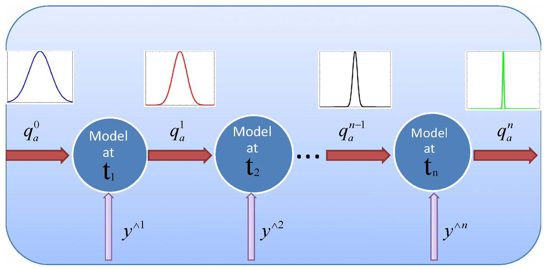
3.2. Sequential Gauss-Markov-Kalman Filter

The process of updating can be done several times on the whole time interval. Once a high non-linear system is divided to very small time steps, the problem turns to plenty of continuous linear systems so that the GMKF approach can update the model parameters in a much better way if it is applied several times to update the model parameters on each time step. Eventually this approach helps to update the uncertain parameters of a non-linear system. Therefore the Gauss-Markov-Kalman filter as in Equation (16) can be written as like in Equation (17) on the k-th time step for the n total time steps, where the Kalman gain reads ${\mathit{K}}^{\left(k\right)}:=\mathrm{cov}({\mathit{q}}_f^{\left(k\right)},y^{\left(k\right)}){(\mathrm{cov}\left(y^{\left(k\right)}\right)+\mathrm{cov}\left(ϵ\right))}^{†}$.

$${{\displaystyle \mathit{q}}}_a^{\left(k\right)}\left(\omega \right)={{\displaystyle \mathit{q}}}_a^{(k-1)}\left(\omega \right)+{{\displaystyle \mathit{K}}}^{\left(k\right)}({\widehat{y}}^{\left(k\right)}-y^{\left(k\right)}\left(\omega \right))$$

(17)

The Equation (17) is called sequential Gauss-Markov-Kalman filter. Schematically the process of sequential Gauss-Markov-Kalman filter is shown in Figure 1 where the posterior of one update is the prior of the next update.

3.3. Numerical Realization

The approaches such as sampling and spectral approximation or functional approximations to compute the linear filter approximations are discussed in this section.

3.3.1. Sampling

Considering N random variables an ensemble of sampling points $\mathit{\omega }=[{\omega }_1,...,{\omega }_N]$ are taken into account [89]. The Gauss-Markov-Kalman filter as shown in Equation (16) for the considered ensemble of sampling points results in Equation (18).

$$\forall \ell =1,...,N:{{\displaystyle \mathit{q}}}_a\left({\omega }_{\ell }\right)={{\displaystyle \mathit{q}}}_f\left({\omega }_{\ell }\right)+{{\displaystyle \mathit{C}}}_{{\mathit{q}}_{f}y}{({{\displaystyle \mathit{C}}}_y+{{\displaystyle \mathit{C}}}_{ϵ})}^{†}(\check{y}-y\left({\omega }_{\ell }\right))$$

(18)

The Equation (18) is the basis of ensemble Gauss-Markov-Kalman filter where ${\mathit{C}}_{{\mathit{q}}_{f}y}=\mathrm{cov}({\mathit{q}}_f,y)$, ${\mathit{C}}_y=\mathrm{cov}\left(y\right)$ and ${\mathit{C}}_{ϵ}=\mathrm{cov}\left(ϵ\right)$. ${\mathit{q}}_f\left({\omega }_l\right)$ and ${\mathit{q}}_a\left({\omega }_l\right)$ are shown as particles in the extended version.

3.3.2. Functional Approximation

The discretization of the random variables are performed by spectral or functional approximations instead of sampling [91,92]. Hence the desired random variables are described as functions of known random variables $\{{\theta }_1\left(\omega \right),...,{\theta }_l\left(\omega \right),...\}$. As only finite random variables can be dealt, a finite vector random variables in functional representation $\mathit{\theta }\left(\omega \right)=[{\theta }_1\left(\omega \right),...,{\theta }_n\left(\omega \right)]$ can be considered where n random variables $\mathit{\theta }$ are taken into account.

The polynomial chaos expansion [93,94] is chosen as system of functions but also other possibilities exist. It should be noted that the finite set of linear independent Hermite functions ${\left\{H_{\alpha }\right\}}_{\alpha \in {\mathcal{J}}_M}$ of variables $\mathit{\theta }\left(\omega \right)$ should include all the linear functions of $\mathit{\theta }$ with polynomials such as polynomial chaos expansion [78]. The multi-index is represented by $\alpha$ and the set ${\mathcal{J}}_M$ is a finite set with cardinality M. The functional approximation of a random variable $\mathit{q}\left(\omega \right)$ is shown in Equation (19).

$${\displaystyle \mathit{q}}\left(\omega \right)=\sum _{\alpha \in {\mathcal{J}}_M}{{\displaystyle \mathit{q}}}_{\alpha }{H}_{\alpha }\left({\displaystyle \mathit{\theta }}\left(\omega \right)\right)=\sum _{\alpha \in {\mathcal{J}}_M}{{\displaystyle \mathit{q}}}_{\alpha }{H}_{\alpha }\left({\displaystyle \mathit{\theta }}\right)={\displaystyle \mathit{q}}\left({\displaystyle \mathit{\theta }}\right)$$

(19)

The argument $\omega$ is neglected in the Equation (19) because the probability measure $\mathbb{P}$ on $\Omega$ is transported to $\mathit{\Theta }={\Theta }_1\times ...\times {\Theta }_n$. The range of $\mathit{\theta }$ showing ${\mathbb{P}}_{\theta }={\mathbb{P}}_1\times ...\times {\mathbb{P}}_n$ as a product measure, where ${\mathbb{P}}_{\ell }={\left({\theta }_{\ell }\right)}_{*}\mathbb{P}$ is the distribution measure of the random variable ${\theta }_{\ell }$ and it is noted that the random variables ${\theta }_{\ell }$ are independent. Therefore all computations are performed on $\mathit{\Theta }$ which is typically a subset of ${\mathbb{R}}^n$. Hence the Gauss-Markov-Kalman filter as shown in Equation (16) for the considered expansion results in Equation (20) which is known as spectral Gauss-Markov-Kalman filter.

$${{\displaystyle \mathit{q}}}_a\left({\displaystyle \mathit{\theta }}\right)={{\displaystyle \mathit{q}}}_f\left({\displaystyle \mathit{\theta }}\right)+{{\displaystyle \mathit{C}}}_{{\mathit{q}}_{f}y}{({{\displaystyle \mathit{C}}}_y+{{\displaystyle \mathit{C}}}_{ϵ})}^{†}(\check{y}-y\left({\displaystyle \mathit{\theta }}\right))={{\displaystyle \mathit{q}}}_f\left({\displaystyle \mathit{\theta }}\right)+{\displaystyle \mathit{K}}(\check{y}-y\left({\displaystyle \mathit{\theta }}\right))$$

(20)

It should also be noted that in spectral approximation the Gauss-Markov-Kalman filter as shown in the Equation (16) has the same form as of the sampling approach but the only difference is the functional approximation of random variables, i.e., the Hermite functions are used to calculate the covariance matrices. For instance ${\mathit{C}}_{{\mathit{q}}_{f}y}$ can be easily computed as given in Equation (21).

$${{\displaystyle \mathit{C}}}_{{\mathit{q}}_{f}y}=\sum _{\alpha >0}\alpha !\left({{\displaystyle \mathit{q}}}_f^{\left(\alpha \right)}\left({\displaystyle \mathit{\theta }}\right)\right){\left(y^{\left(\alpha \right)}\left({\displaystyle \mathit{\theta }}\right)\right)}^T$$

(21)

While the Equation (16) is applied on samples or particles in sampling approach, in spectral approximations it is applied on the coefficients as shown in Equation (19) which are the functional approximation of the random variables.

4. Numerical Results

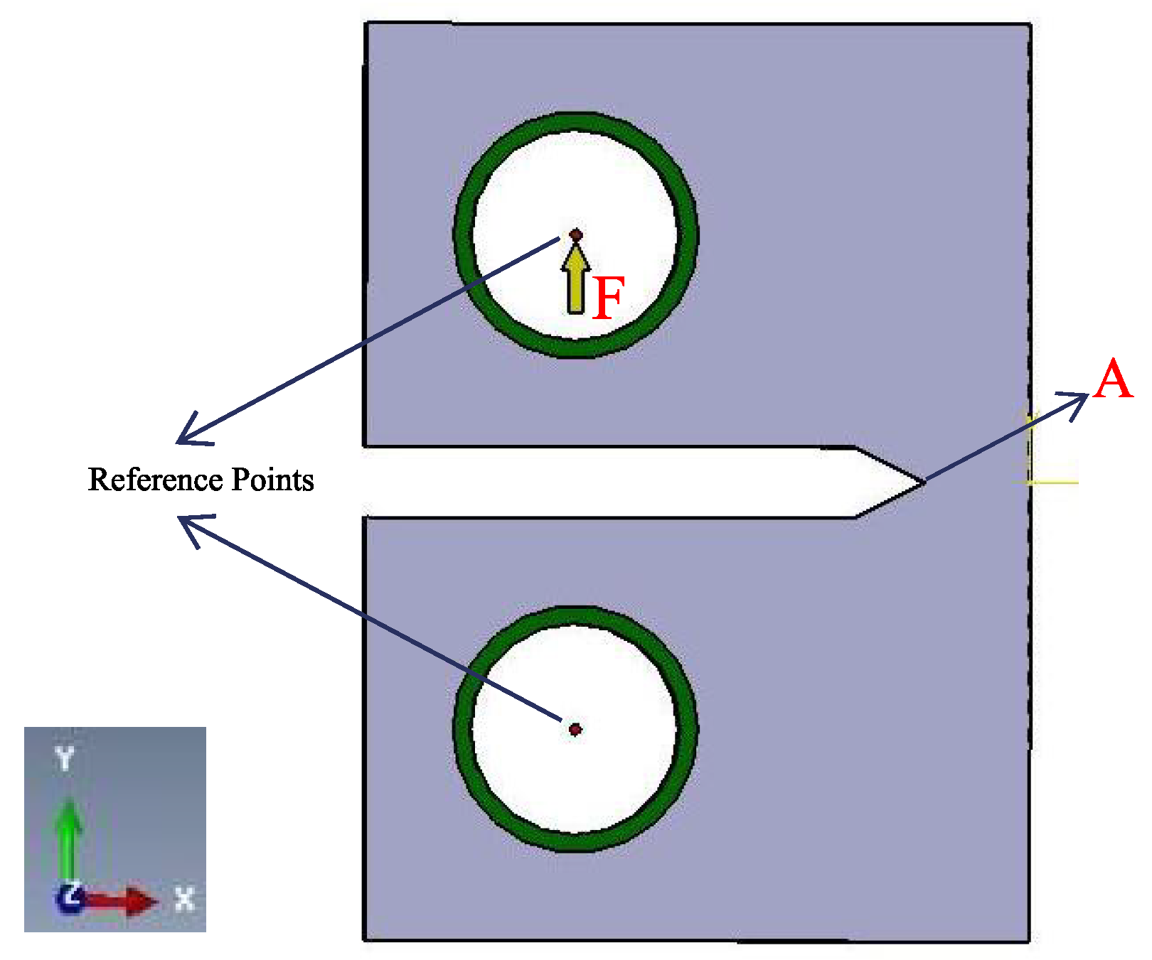
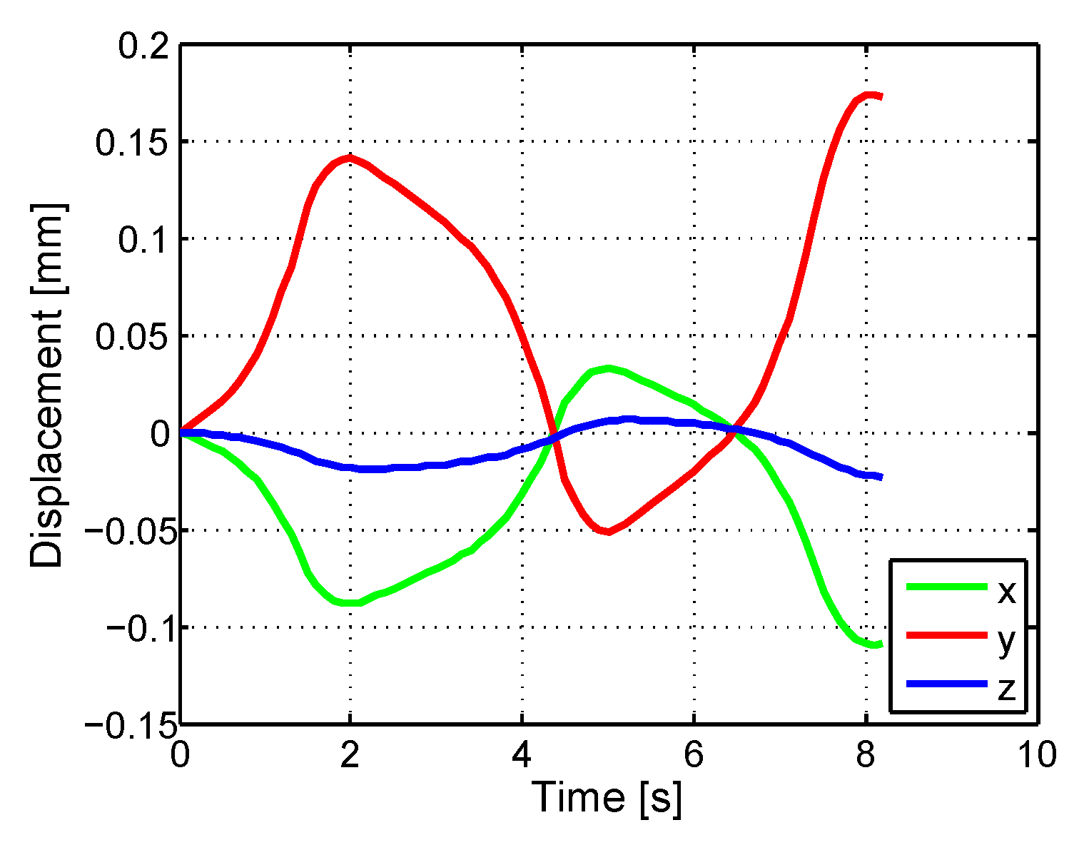
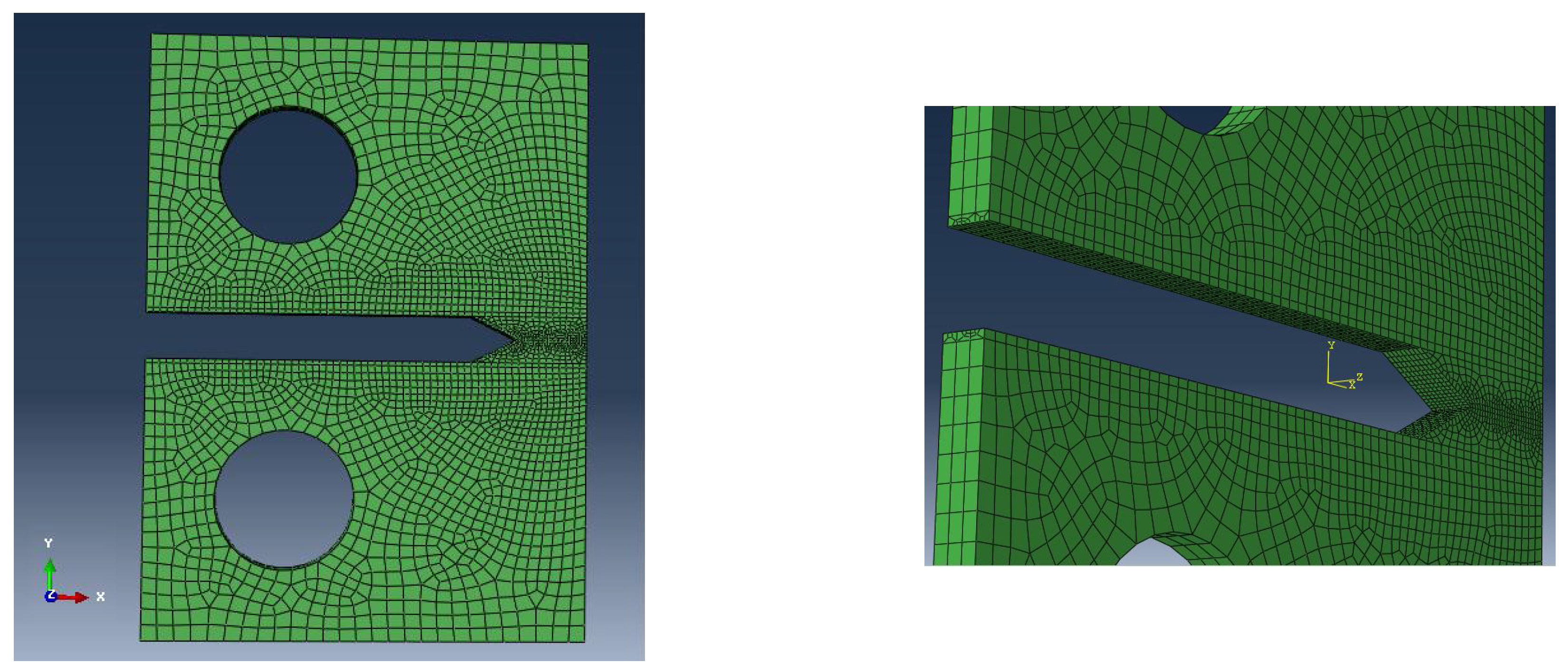
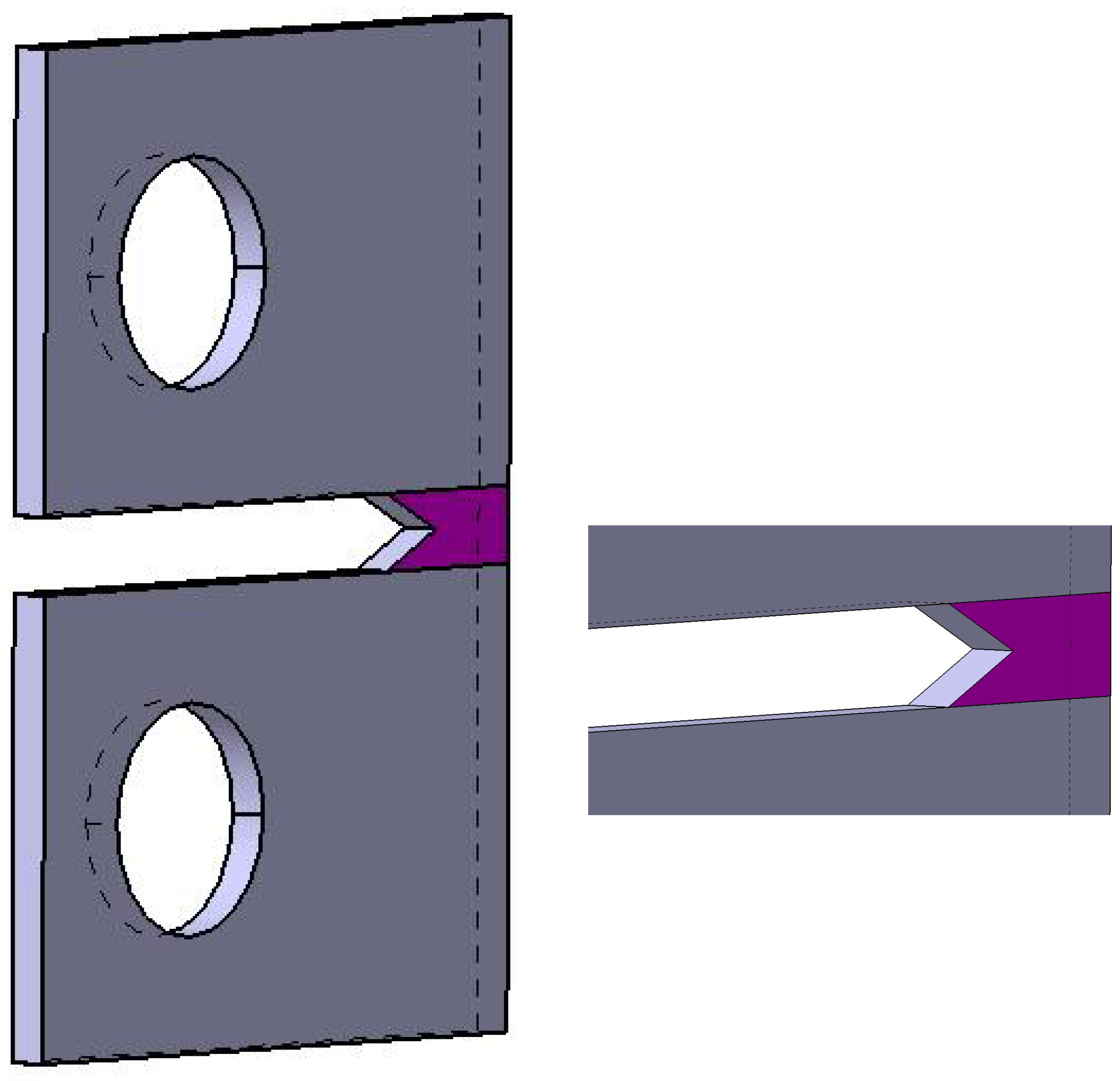
The identification of the material constants in the Chaboche unified viscoplasticity model with damage is a reverse process based on virtual data. The aim of the parameter estimation is to find a parameter vector q introduced in the previous section. The bulk modulus ($\nleqq$), the shear modulus (G), the isotropic hardening coefficient ($b_R$), the kinematic hardening coefficient ($b_{\chi }$) and the yield stress (${\sigma }_y$) as well as damage parameters ($c_1$, $c_2$ and $c_3$) are considered as uncertain parameters of the constitutive model.

As both kinds of hardenings are taken into account and the studied model is a damaged material model one appropriate way of the identification of parameters is to use the results of the cyclic tests as observation, since more information can be obtained from virtual data rather than from creep and relaxation tests, especially information regarding hardening and damage parameters as the hardening and damage equations are involved in this case.

CT-Test

In the following of our previous studies [77,95,96,97], a very well-known Compact Tension Test (CT-Test) [98] is carried out on a notched sample. The Dirichlet boundary condition is applied by assigning two reference points at the center of two holes of the specimen as seen in Figure 2.

The reference points are kinematically coupled with the corresponding holes. The displacement of the reference point at upper hole is constrained in x and z directions and the displacement of reference point at the lower hole is constrained in x, y and z directions. Moreover, to depict a soft transition of the constraints in the specimen the first layer of the elements around the holes are defined with much softer material than the rest of the elements. The first layer of the elements around the holes are shown in green color in Figure 2. As a Neumann boundary condition, a cyclic load in y-direction is applied on the reference point of the upper hole as shown with a yellow arrow in Figure 2.

The load is applied in such a way that the damage parameter does not exceed relatively small amount, so that it will not probably result in a severe damage or collapsing damage. The minor damage or light cracking is only developed to identify the model parameters in the Bayesian setting so that it can be later used for health monitoring purpose where identifying the model parameters and detecting the damage before collapsing the specimen is a crucial issue.

From the above discussion, considered boundary conditions and the parameters as seen in

Table 2. The model parameters.

	$\mathit{\kappa }$	G	${\mathit{\sigma }}_{\mathit{y}}$	n	k	${\mathit{b}}_{\mathit{R}}$	${\mathit{H}}_{\mathit{R}}$	${\mathit{b}}_{\mathit{\chi }}$
$H_{\chi }$	$c_1$	$c_2$	$c_3$	$c_4$	$c_5$
	$1.66\times {10}^5$	$7.69\times {10}^4$	266	1	$23,500$	$298.6$	$117.2$	100
150	$4.5$	5	$-11$	15	$3.75$

, the related displacement graph as shown in Figure 3 was obtained where green, red and blue colors represent the displacement of the node in x, y, and z directions respectively at the notch start point indicated by point A in Figure 2.

The mesh generated for the CT-Test model is shown in Figure 4, where the meshes are generated in such a way that the very fine meshes are considered near the notch and at far away from the notch coarser meshes are generated. Further, Figure 5 shows the damaged specimen.

The displacement of the nodes on the external surface close to the notch which is seen in Figure 6 are recorded. Some Gaussian white noise like the observed displacement over time is added to the output data to have a perturbed virtual data. In order to consider the model error, data is determined for a full damage model introduced in Section 2 but the parameters are identified for a model with different damage equation as shown in Equation (22).

$$\dot{D}=(c_1+c_2{e}^{-c_3{p}^{+}}){\dot{p}}^{+}$$

(22)

These mentioned changes not only results in a very ill-posed problem but proves the applicability of the Gauss-Markov-Kalman filter method on different studied models, i.e., the data model and the identification model, which indeed represents an artificial model error.

Applying stochastic identification which is fully discussed in Section 3, the probability density function of prior and posterior of the identified parameters can be seen in Figure 7.

Summarizing the results, the true values and the mean and variance of the estimated parameters are compared in

Table 3. The identified model parameters.

Parameters	${\mathit{q}}_{\mathbf{true}}$	${\mathit{q}}_{\mathbf{est}}\left(\mathbf{Mean}\right)$	${\mathit{q}}_{\mathbf{est}}\left(\mathbf{Standard}\mathbf{Deviation}\right)$
$\kappa$	$1.66\times {10}^5$	$1.66\times {10}^5$	$255.73$
G	$7.69\times {10}^4$	$7.69\times {10}^4$	$34.55$
${\sigma }_y$	266	$265.99$	$0.51$
$b_R$	298.6	298.57	0.51
$b_{\chi }$	100	100.0	1.19
$c_1$	4.5	4.46	0.21
$c_2$	5	5.04	0.20
$c_3$	−11	−10.97	0.25

.

5. Discussion and Comparison

The parameters such as bulk modulus ($\kappa$), shear modulus (G) and yield stress (${\sigma }_y$) are even identified after updating once as the effect of these parameters on the equation of the displacement are much higher than the rest of the parameters and it is very expensive to update the uncertainty distribution on each time step. Hence the parameters are updated not in elastic states but only in the plastic states where the bulk modulus ($\kappa$), shear modulus (G), yield stress (${\sigma }_y$), hardening parameters (($b_R$) and ($b_{\chi }$)) and damage parameters (($c_1$), ($c_2$) and ($c_3$)) can be updated as updating in the elastic states increases the cost. The evaluation of hardening and local damage on the top node at the notch start point representing the plasticity are shown in Figure 8. In order to reduce the time of computation, the displacements of nodes are sequentially updated only in the time intervals $\left[0.42.2\right]$, $\left[3.55.0\right]$ and $\left[6.68.2\right]$. Although all the nodes do not have the same evaluation of hardening and local damage but with a good approximation the nodes considered on the mentioned surfaces for the both cases have the quite close hardening and damage behaviors on the determined time interval and therefore updating is only done within these time intervals.

The other fact that should be emphasized is that the observed displacement is directly influenced by the bulk modulus ($\kappa$), shear modulus (G), and yield stress (${\sigma }_y$) as in $u\propto \mathsf{f}(\kappa ,G,{\sigma }_y)$, i.e., these parameters have a direct strong effect on the measured displacement. The rest of the parameters affect the displacement as in $u\propto \mathsf{f}\left(\mathsf{g}\left(\mathsf{k}(b_R,b_{\chi },c_1,c_2,c_3)\right)\right)$, i.e., the displacement is proportional to these parameters through some more functions. Accordingly, the information received from the constitutive equation from the latter parameters are less and therefore they can not be generally estimated as good as the first group of parameters. However the hardening parameters for both cases are also updated well as a lot of nodes’ displacements are observed and considered as the measurement data.

The bulk modulus, shear modulus and yield stress are updated much easier than the hardening and damage parameters as enough information from the virtual data are received and this was observed from the sharpness of posterior probability density function of bulk modulus ($\kappa$), shear modulus (G), and yield stress (${\sigma }_y$). However the hardening parameters (($b_R$) and ($b_{\chi }$)) are also very well updated for this case study as large numbers of measurements are considered which provide good enough information to estimate hardening parameters using sequential Gauss-Markov-Kalman filter approach. It also can be inferred that number of observation data which is here the number of nodes that their output displacements are considered as the measurement data plays a very significant role. In other words, by having more measurement data a good enough identification is possible, as the standard deviations of the residual uncertainties are below $5\%$ of their mean values, even if the data and identification model are different.

The identified parameters of the CT-Test are also compared with the updated parameters of a 8 node element as in [77] and it is found that since for CT-Test more nodes are observed and their displacements are measured but for the 8 node element only one node is observed, the parameters are identified better especially the damage parameters (($c_1$), ($c_2$) and ($c_3$)) for the CT-Test. Moreover, for the CT-Test, the standard deviation of parameters representing the uncertainty are updated more than the one element test and their probability density functions are narrowed much more for the CT-Test.

6. Summary

In this paper, a sequential Gauss-Markov-Kalman filter approach is applied on a viscoplastic-damage model on a well-known test, so-called CT-Test in order to identify its model parameters. The conclusion from the discussions and comparisons are classified below.

• The sequential Gauss-Markov-Kalman filter approach can be applied to update the model parameters by considering the surface displacement as the measurement data. The better identification and better reduction in uncertainties of the parameters is achieved by considering more number of nodes.
• The number of updating can be reduced to reduce the computation time when more information from the large number of nodal displacement is available. The CT-Test with a very fine mesh takes a lot of time to solve the system of PDE, therefore updating is performed only at few certain time steps and these time steps should be chosen smartly in a way as discussed in Section 4. The sequential Gauss-Markov-Kalman filter approach updates the model parameters properly where updatings are done on some specified time steps by considering a large observation data available from the surface strain.
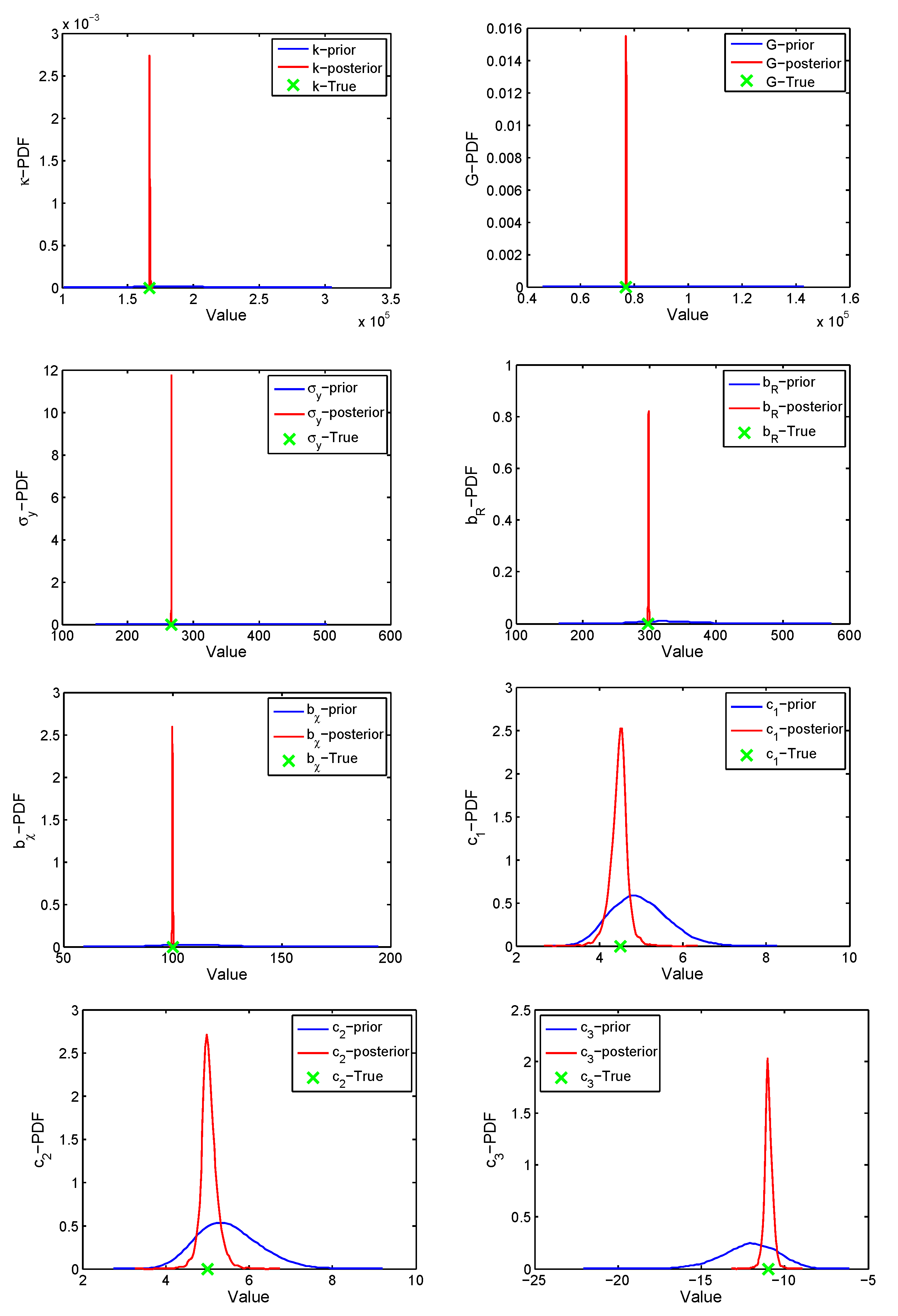
• Considering the model error by taking into account different data model and identification model, the sequential Gauss-Markov-Kalman filter approach can still be employed to identify the model parameters by considering the large number of measurement data determined from the surface displacement of a different data model as the parameters are identified properly. The estimated parameters are very close to the true values as shown in Table 3.

Considering the above mentioned comparisons, observations, discussions and results, it can be concluded that identification of model parameters is possible using sequential Gauss-Markov-Kalman filter approach from pure surface measurement of strain which is practically possible in the form of Digital Image Correlation (DIC). Hence this approach can also be used for the health monitoring purposes as the model parameters can be estimated before the occurrence of severe damage and collapse [80].

References

1. Miller, A. An inelastic constitutive model for monotonic, cyclic, and creep deformation: Part I–equations development and analytical procedures. J. Eng. Mater. Technol. 1976, 98, 97–105. [Google Scholar] [CrossRef]
2. Krempl, E.; McMahon, J.J.; Yao, D. Viscoplasticity based on overstress with a differential growth law for the equilibrium stress. J. Mech. Mater. 1986, 5, 35–48. [Google Scholar] [CrossRef] [Green Version]
3. Korhonen, R.K.; Laasanen, M.S.; Toyras, J.; Lappalainen, R.; Helminen, H.J.; Jurvelin, J.S. Fibril reinforced poroelastic model predicts specifically mechanical behavior of normal, proteoglycan depleted and collagen degraded articular cartilage. J. Biomech. 2003, 36, 1373–1379. [Google Scholar] [CrossRef]
4. Aubertin, M.; Gill, D.E.; Ladanyi, B. A unified viscoplastic model for the inelastic flow of alkali halides. J. Mech. Mater. 1991, 11, 63–82. [Google Scholar] [CrossRef]
5. Chan, K.S.; Bodner, S.R.; Fossum, A.F.; Munson, D.E. A constitutive model for inelastic flow and damage evolution in solids under triaxial compression. J. Mech. Mater. 1992, 14, 1–14. [Google Scholar] [CrossRef]
6. Chaboche, J.L.; Rousselier, G. On the plastic and viscoplastic constitutive equations—Part 1: Rules developed with internal variable concept. J. Press. Vessel Technol. 1983, 105, 153–158. [Google Scholar] [CrossRef]
7. Chaboche, J.L.; Rousselier, G. On the plastic and viscoplastic constitutive equations—Part 2: Application of internal variable concepts to the 316 stainless steel. J. Press. Vessel Technol. 1983, 105, 159–164. [Google Scholar] [CrossRef]
8. An, D.; Cho, J.; Kim, N.H. Identification of correlated damage parameters under noise and bias using Bayesian inference. Struct. Health Monit. 2011, 11, 293–303. [Google Scholar] [CrossRef]
9. Hernandez, W.P.; Borges, F.C.L.; Castello, D.A.; Roitman, N.; Magluta, C. Bayesian inference applied on model calibration of a fractional derivative viscoelastic model. In Proceedings of the XVII International Symposium on Dynamic Problems of Mechanics, Natal, Brazil, 22–27 February 2015. [Google Scholar]
10. Mahnken, R. Identification of material parameters for constitutive equations. In Encyclopedia of Computational Mechanics Second Edition, Part 2. Solids and Structures; Wiley: Hoboken, NJ, USA, 2017; pp. 1–21. [Google Scholar]
11. Zheng, W.; Yu, Y. Bayesian probabilistic framework for damage identification of steel truss bridges under joint uncertainties. Adv. Civ. Eng. 2013, 2013, 1–13. [Google Scholar] [CrossRef]
12. Nichols, J.M.; Moore, E.Z.; Murphy, K.D. Bayesian identification of a cracked plate using a population-based Markov Chain Monte Carlo method. J. Comput. Struct. 2011, 89, 1323–1332. [Google Scholar] [CrossRef]
13. Madireddy, S.; Sista, B.; Vemaganti, K. A Bayesian approach to selecting hyperelastic constitutive models of soft tissue. J. Comput. Appl. Math. 2015, 291, 102–122. [Google Scholar] [CrossRef]
14. Wang, J.; Zabaras, N. A Bayesian inference approach to the inverse heat conduction problem. Int. J. Heat Mass Transf. 2004, 47, 3927–3941. [Google Scholar] [CrossRef]
15. Oh, C.K.; Beck, J.L.; Yamada, M. Bayesian learning using automatic relevance determination prior with an application to earthquake early warning. J. Eng. Mech. 2008, 134, 1013–1020. [Google Scholar] [CrossRef] [Green Version]
16. Alvin, K. Finite element model update via Bayesian estimation and minimization of dynamic residuals. Am. Inst. Aeronaut. Astronaut. J. 1997, 135, 879–886. [Google Scholar] [CrossRef] [Green Version]
17. Marwala, T.; Sibusiso, S. Finite element model updating using Bayesian framework and modal properties. J. Aircr. 2005, 42, 275–278. [Google Scholar] [CrossRef]
18. Daghia, F.; de Miranda, S.; Ubertini, F.; Viola, E. Estimation of elastic constants of thick laminated plates within a Bayesian framework. J. Compos. Struct. 2007, 80, 461–473. [Google Scholar] [CrossRef]
19. Abhinav, S.; Manohar, C. Bayesian parameter identification in dynamic state space models using modified measurement equations. Int. J. Non-Linear Mech. 2015, 71, 89–103. [Google Scholar] [CrossRef]
20. Gogu, C.; Yin, W.; Haftka, R.; Ifju, P.; Molimard, J.; le Riche, R.; Vautrin, A. Bayesian identification of elastic constants in multi-directional laminate from Moire interferometry displacement fields. J. Exp. Mech. 2013, 53, 635–648. [Google Scholar] [CrossRef] [Green Version]
21. Gogu, C.; Haftka, R.; Molimard, J.; Vautrin, A. Introduction to the Bayesian approach applied to elastic constants identification. Am. Inst. Aeronaut. Astronaut. J. 2010, 48, 893–903. [Google Scholar] [CrossRef]
22. Koutsourelakis, P.S. A novel Bayesian strategy for the identification of spatially varying material properties and model validation: An application to static elastography. Int. J. Numer. Methods Eng. 2012, 91, 249–268. [Google Scholar] [CrossRef] [Green Version]
23. Koutsourelakis, P.S. A multi-resolution, non-parametric, Bayesian framework for identification of spatially-varying model parameters. J. Comput. Phys. 2009, 228, 6184–6211. [Google Scholar] [CrossRef] [Green Version]
24. Fitzenz, D.D.; Jalobeanu, A.; Hickman, S.H. Integrating laboratory creep compaction data with numerical fault models: A Bayesian framework. J. Geophys. Res. Solid Earth 2007, 112, B08410. [Google Scholar] [CrossRef]
25. Most, T. Identification of the parameters of complex constitutive models: Least squares minimization vs. Bayesian updating. In Reliability and Optimization of Structural Systems; Straub, D., Ed.; CRC Press: Boca Raton, FL, USA, 2010; pp. 119–130. [Google Scholar]
26. Sarkar, S.; Kosson, D.S.; Mahadevan, S.; Meeussen, J.C.L.; Sloot, H.v.; Arnold, J.R.; Brown, K.G. Bayesian calibration of thermodynamic parameters for geochemical speciation modeling of cementitious materials. J. Cem. Concr. Res. 2012, 42, 889–902. [Google Scholar] [CrossRef]
27. Zhang, E.; Chazot, J.D.; Antoni, J.; Hamdi, M. Bayesian characterization of Young’s modulus of viscoelastic materials in laminated structures. J. Sound Vib. 2013, 332, 3654–3666. [Google Scholar] [CrossRef]
28. Mehrez, L.; Kassem, E.; Masad, E.; Little, D. Stochastic identification of linear-viscoelastic models of aged and unaged asphalt mixtures. J. Mater. Civ. Eng. 2015, 27, 04014149. [Google Scholar] [CrossRef]
29. Miles, P.; Hays, M.; Smith, R.; Oates, W. Bayesian uncertainty analysis of finite deformation viscoelasticity. J. Mech. Mater. 2015, 91, 35–49. [Google Scholar] [CrossRef] [Green Version]
30. Zhao, X.; Pelegri, A.A. A Bayesian approach for characterization of soft tissue viscoelasticity in acoustic radiation force imaging. Int. J. Numer. Methods Biomed. Eng. 2016, 32, E02741. [Google Scholar] [CrossRef]
31. Kenz, Z.R.; Banks, H.T.; Smith, R.C. Comparison of frequentist and Bayesian confidence analysis methods on a viscoelastic stenosis model. SIAM/ASA J. Uncertain. Quantif. 2013, 1, 348–369. [Google Scholar] [CrossRef] [Green Version]
32. An, D.; Choi, J.; Kim, N.H.; Pattabhiraman, S. Fatigue life prediction based on Bayesian approach to incorporate field data into probability model. J. Struct. Eng. Mech. 2011, 37, 427–442. [Google Scholar] [CrossRef] [Green Version]
33. Wang, C.; Qiu, Z.; Wang, X.; Wu, D. Interval finite element analysis and reliability-based optimization of coupled structural-acoustic system with uncertain parameters. Finite Elem. Anal. Des. 2014, 91, 108–114. [Google Scholar] [CrossRef]
34. Hoshi, T.; Kobayashi, Y.; Kawamura, K.; Fujie, M.G. Developing an intraoperative methodology using the finite element method and the extended Kalman filter to identify the material parameters of an organ model. In Proceedings of the 29th Annual International Conference of the IEEE EMBS Cité Internationale, Lyon, France, 23–26 August 2007. [Google Scholar]
35. Furukawa, T.; Pan, J.W. Stochastic identification of elastic constants for anisotropic materials. Int. J. Numer. Methods Eng. 2010, 81, 429–452. [Google Scholar] [CrossRef]
36. Conte, J.P.; Astroza, R.; Ebrahimian, H. Bayesian methods for nonlinear system identification of civil structures. MATEC Web Conf. 2015, 24, 03002. [Google Scholar] [CrossRef]
37. Hendriks, M.A.N. Identification of the Mechanical Behavior of Solid Materials. Ph.D. Dissertation, Department of Mechanical Engineering, Technische Universiteit Eindhoven, Eindhoven, The Netherlands, 1991. [Google Scholar]
38. Bolzon, G.; Fedele, R.; Maier, G. Parameter identification of a cohesive crack model by Kalman filter. J. Comput. Methods Appl. Mech. Eng. 2002, 191, 2847–2871. [Google Scholar] [CrossRef]
39. Mahmoudi, E.; König, M. Reliability-based robust design optimization of rock salt cavern. In Proceedings of the 29th European Safety and Reliability Conference, Hannover, Germany, 22–26 September 2019. [Google Scholar]
40. Mahmoudi, E.; Hölter, R.; Zhao, C.; Datcheva, M. System Identification concepts to explore mechanised tunnelling in urban areas. In Proceedings of the Dritte Deutesche Bodenmechaniktagung, Bochum, Germany, February 2019. [Google Scholar]
41. Wall, O.; Holst, J. Estimation of parameters in viscoplastic and creep material models. SIAM J. Appl. Math. 2001, 61, 2080–2103. [Google Scholar] [CrossRef]
42. Nakamura, T.; Gu, Y. Identification of elastic-plastic anisotropic parameters using instrumented indentation and inverse analysis. J. Mech. Mater. 2007, 39, 340–356. [Google Scholar] [CrossRef]
43. Agmell, M.; Ahadi, A.; Stahl, J. Identification of plasticity constants from orthogonal cutting and inverse analysis. J. Mech. Mater. 2014, 77, 43–51. [Google Scholar] [CrossRef]
44. Sevieri, G.; Andreini, M.; Falco, A.D.; Matthies, H.G. Concrete gravity dams model parameters updating using static measurements. Eng. Struct. 2019, 196, 109231. [Google Scholar] [CrossRef]
45. Sevieri, G.; Falco, A.D. Dynamic structural health monitoring for concrete gravity dams based on the Bayesian inference. J. Civ. Struct. Health Monit. 2020, 10, 235–250. [Google Scholar] [CrossRef] [Green Version]
46. Sevieri, G.; Falco, A.D.; Marmo, G. Shedding Light on the Effect of Uncertainties in the Seismic Fragility Analysis of Existing Concrete Dams. Infrastructures 2020, 5, 22. [Google Scholar] [CrossRef] [Green Version]
47. Marsili, F.; Croce, P.; Friedman, N.; Formichi, P.; Landi, F. Seismic reliability assessment of a concrete water tank based on the Bayesian updating of the finite element model. ASCE-ASME J. Risk Uncertain. Eng. Syst. Part B Mech. Eng. 2017, 3, 021004. [Google Scholar] [CrossRef]
48. Marsili, F.; Croce, P.; Friedman, N.; Formichi, P.; Landi, F. On Bayesian identification methods for the analysis of existing structures. In Proceedings of the IABSE Congress Stockholm, Challenges in Design and Construction of an Innovative and Sustainable Built Environment, Stockholm, Sweden, 21–23 September 2016; pp. 116–123. [Google Scholar]
49. Croce, P.; Landi, F.; Formichi, P. Probabilistic Seismic Assessment of Existing Masonry Buildings. Buildings 2019, 9, 237. [Google Scholar] [CrossRef] [Green Version]
50. Croce, P.; Formichi, P.; Landi, F. A Bayesian hierarchical model for climatic loads under climate change. Eccomas Proceedia UNCECOMP 2019, 298–308. [Google Scholar] [CrossRef] [Green Version]
51. Croce, P.; Marsili, F.; Klawonn, F.; Formichi, P.; Landi, F. Evaluation of statistical parameters of concrete strength from secondary experimental test data. Constr. Build. Mater. 2018, 163, 343–359. [Google Scholar] [CrossRef]
52. Hariri-Ardebili, M.A.; Sudret, B. Polynomial chaos expansion for uncertainty quantification of dam engineering problems. Eng. Struct. 2020, 203, 109631. [Google Scholar] [CrossRef]
53. Hariri-Ardebili, M.A.; Heshmati, M.; Boodagh, P.; Salamon, J.W. Probabilistic Identification of Seismic Response Mechanism in a Class of Similar Arch Dams. Infrastructures 2019, 4, 44. [Google Scholar] [CrossRef] [Green Version]
54. Saouma, V.E.; Hariri-Ardebili, M.A. Probabilistic Cracking, Aging and Shaking of Concrete Dams. In Proceedings of the 5th International Symposiumon Dam Safety, Istanbul, Turkey, 27–31 October 2018; pp. 44–56. [Google Scholar]
55. Pouraminian, M.; Pourbakhshian, S.; Hosseini, M.M. Reliability Analysis of Pole Kheshti Historical Arch Bridge under Service Loads using SFEM. J. Build. Pathol. Rehabil. 2019, 4, 21. [Google Scholar] [CrossRef]
56. Pouraminian, M.; Pourbakhshian, S.; Farasangi, E.N.; Fotoukian, R. Probabilistic Safety Evaluation of a Concrete Arch Dam Based on Finite Element Modeling and a Reliability L-R Approach. Civ. Environ. Eng. Rep. 2019, 29, 62–78. [Google Scholar] [CrossRef] [Green Version]
57. Pouraminian, M.; Pourbakhshian, S.; Farasangi, E.N. Reliability Assessment and Sensitivity Analysis of Concrete Gravity Dams by Considering Uncertainty in Reservoir Water Levels and Dam Body Materials. Civ. Environ. Eng. Rep. 2020, 30, 1–17. [Google Scholar] [CrossRef]
58. Ghannadi, P.; Kourehli, S.S. Model updating and damage detection in multi-story shear frames using salp swarm algorithm. Earthquakes Struct. 2019, 17, 63–73. [Google Scholar]
59. Ghannadi, P.; Kourehli, S.S.; Noori, M.; Altabey, W.A. Efficiency of grey wolf optimization algorithm for damage detection of skeletal structures via expanded mode shapes. Adv. Struct. Eng. 2020. [Google Scholar] [CrossRef]
60. Gharehbaghi, V.; Nguyen, A.; Farsangi, E.N.; Yang, T.Y. Supervised damage and deterioration detection in building structures using an enhanced autoregressive time-series approach. J. Build. Eng. 2020. [Google Scholar] [CrossRef]
61. Bocciarelli, M.; Bolzon, G.; Maier, G. A constitutive model of metal-ceramic functionally graded material behavior: Formulation and parameter identification. J. Comput. Mater. Sci. 2008, 43, 16–26. [Google Scholar] [CrossRef]
62. Gu, Y.; Nakamura, T.; Prchlik, L.; Sampath, S.; Wallace, J. Micro-indentation and inverse analysis to characterize elastic-plastic graded materials. J. Mater. Sci. Eng. A 2003, 345, 223–233. [Google Scholar] [CrossRef]
63. Corigliano, A.; Mariani, S. Parameter identification of a time-dependent elastic-damage interface model for the simulation of debonding in composites. J. Compos. Sci. Technol. 2001, 61, 191–203. [Google Scholar] [CrossRef]
64. Corigliano, A.; Mariani, S. Simulation of damage in composites by means of interface models: Parameter identification. J. Compos. Sci. Technol. 2001, 61, 2299–2315. [Google Scholar] [CrossRef]
65. Ebrahimian, H.; Astroza, R.; Conte, J.P.; de Callafon, R.A. Nonlinear finite element model updating for damage identification of civil structures using batch Bayesian estimation. J. Mech. Syst. Signal Process. 2017, 84, 194–222. [Google Scholar] [CrossRef]
66. Ebrahimian, H.; Astroza, R.; Conte, J.P. Parametric Identification of Hysteretic Material Constitutive Laws in Nonlinear Finite Element Models Using Extended Kalman Filter; Department of Structural Engineering, University of California: La Jolla, San Diego, CA, USA, 2014. [Google Scholar]
67. Ebrahimian, H.; Astroza, R.; Conte, J.P. Extended Kalman filter for material parameter estimation in nonlinear structural finite element models using direct differentiation method. Earthq. Eng. Struct. Dyn. 2015, 44, 1495–1522. [Google Scholar] [CrossRef]
68. Astroza, R.; Ebrahimian, H.; Conte, J.P. Material parameter identification in distributed plasticity FE models of frame-type structures using nonlinear stochastic filtering. J. Eng. Mech. 2015, 141, 04014149. [Google Scholar] [CrossRef]
69. Yan, A.; de Boe, P.; Golinval, J. Structural damage diagnosis by Kalman model based on stochastic subspace identification. Int. J. Struct. Health Monit. 2004, 3, 103–119. [Google Scholar] [CrossRef]
70. Yaghoubi, V.; Marelli, S.; Sudret, B.; Abrahamsson, T. Polynomial chaos expansions for modeling the frequency response functions of stochastic dynamical system. In Proceedings of the European Congress on Computational Methods in Applied Sciences and Engineering, ECCOMAS, Crete, Greece, 5–10 June 2016. [Google Scholar]
71. Yaghoubi, V.; Marelli, S.; Sudret, B.; Abrahamsson, T. Sparse polynomial chaos expansions of frequency response functions using stochastic frequency transformation. Probabilistic Eng. Mech. 2017, 48, 39–58. [Google Scholar] [CrossRef] [Green Version]
72. Yaghoubi, V.; Silani, M.; Zolfaghari, H.; Jamshidian, M.; Rabczuk, T. Nonlinear interphase effects on plastic hardening of nylon 6/clay nanocomposites: A computational stochastic analysis. J. Compos. Mater. 2019, 54, 753–763. [Google Scholar] [CrossRef]
73. Hamdia, K.M.; Silani, M.; Zhuang, X.; He, P.; Rabczuk, T. Stochastic analysis of the fracture toughness of polymeric nanoparticle composites using polynomial chaos expansions. Int. J. Fract. 2017, 206, 215–227. [Google Scholar] [CrossRef]
74. Silani, M.; Talebi, H.; Ziaei-Rad, S.; Kerfriden, P.; Bordas, S.; Rabczuk, T. Stochastic modelling of clay/epoxy nanocomposites. Compos. Struct. 2014, 118, 241–249. [Google Scholar] [CrossRef]
75. Hamdia, K.M.; Msekh, M.A.; Silani, M.; Vu-Bac, N.; Zhuang, X.; Nguyen-Thoi, T.; Rabczuk, T. Uncertainty quantification of the fracture properties of polymeric nanocomposites based on phase field modeling. Compos. Struct. 2015, 133, 1177–1190. [Google Scholar] [CrossRef]
76. Stanisaukis, E.; Solheim, H.; Mashayekhi, S.; Miles, P.; Oates, W. Modeling, experimental characterization, and uncertainty quantification of auxetic foams: Hyperelastic and fractional viscoelastic mechanics. In Proceedings of the Behavior and Mechanics of Multifunctional Materials IX, California, CA, USA, 27 April–8 May 2020. [Google Scholar]
77. Adeli, E.; Rosić, B.V.; Matthies, H.G.; Reinstädler, S.; Dinkler, D. Comparison of Bayesian Methods on Parameter Identification for a Viscoplastic Model with Damage. Metals 2020, 10, 876. [Google Scholar] [CrossRef]
78. Matthies, H.G.; Litvinenko, A.; Rosić, B.V.; Zander, E. Bayesian parameter estimation via filtering and functional approximations. Tech. Gaz. 2016, 23, 1–8. [Google Scholar]
79. Pajonk, O.; Rosić, B.V.; Litvinenko, A.; Matthies, H.G. A deterministic filter for non-Gaussian Bayesian estimation—Applications to dynamical system estimation with noisy measurements. Physica D Nonlinear Phenom. 2012, 241, 775–788. [Google Scholar] [CrossRef]
80. Adeli, E. Viscoplastic-Damage Model Parameter Identification via Bayesian Methods. Ph.D. Thesis, Institut für Wissenschaftliches Rechnen, Technische Universität Braunschweig, Braunschweig, Germany, February 2019. [Google Scholar] [CrossRef]
81. Simo, J.C.; Hughes, T.J.R. Computational Inelasticity, 7th ed.; Springer: New York, NY, USA, 1998. [Google Scholar]
82. Kowalsky, U.; Meyer, J.; Heinrich, S.; Dinkler, D. A nonlocal damage model for mild steel under inelastic cyclic straining. Comput. Mater. Sci. 2012, 63, 28–34. [Google Scholar] [CrossRef]
83. Pirondi, A.; Bonora, N. Modeling ductile damage under fully reversed cycling. Comput. Mater. Sci. 2003, 26, 129–141. [Google Scholar] [CrossRef]
84. Hughes, T.; Hulbert, G. Space-time finite element methods for elastodynamics: Formulations and error estimates. Comput. Methods Appl. Mech. Eng. 1988, 66, 339–363. [Google Scholar] [CrossRef]
85. Zienkiewicz, O.C.; Taylor, R.L.; Zhu, J.Z. The Finite Element Method: Its Basis and Fundamentals, 6th ed.; Elsevier Butterworth-Heinemann: Oxford, UK, 2005; ISBN 978-1-85617-633-0. [Google Scholar]
86. Luenberger, D.G. Optimization by Vector Space Methods; Wiley: Chichester, UK, 1969. [Google Scholar]
87. Grewal, M.S.; Andrews, A.P. Kalman Filtering: Theory and Practice Using MATLAB; Wiley: Chichester, UK, 2008. [Google Scholar]
88. McGrayne, S.B. The Theory that Would Not Die; Yale University Press: New Haven, CT, USA, 2011. [Google Scholar]
89. Evensen, G. Data Assimilation–the Ensemble Kalman Filter; Springer: Berlin, Germany, 2009. [Google Scholar]
90. Pajonk, O. Stochastic Spectral Methods for Linear Bayesian Inference. Ph.D. Dissertation, Institut für Wissenschaftliches Rechnen, Technische Universität Braunschweig, Braunschweig, Germany, February 2012. [Google Scholar]
91. Matthies, H.G. Stochastic finite elements: Computational Approaches to Stochastic Partial Differential Equations. J. Appl. Math. Mech. 2008, 88, 849–873. [Google Scholar] [CrossRef]
92. Xiu, D. Numerical Methods for Stochastic Computations: A Spectral Method Approach; Princeton University Press: Princeton, NJ, USA, 2010. [Google Scholar]
93. Wiener, N. The homogeneous chaos. Am. J. Math. 1938, 60, 897–936. [Google Scholar] [CrossRef]
94. Ghanem, R.; Spanos, P.D. Stochastic Finite Elements—A Spectral Approach; Springer: Berlin, Germany, 1991. [Google Scholar]
95. Adeli, E.; Rosić, B.V.; Matthies, H.G.; Reinstädler, S. Bayesian parameter identification in plasticity. In Proceedings of the XIV International Conference on Computational Plasticity: Fundamentals and Applications COMPLAS XIV, Barcelona, Spain, 5–7 September 2017. [Google Scholar]
96. Adeli, E.; Rosić, B.V.; Matthies, H.G.; Reinstädler, S. Effect of Load Path on Parameter Identification for Plasticity Models using Bayesian Methods. In Lecture Notes in Computational Science and Engineering; Nature Springer: Berlin, Germany, 2018; Available online: http://arxiv.org/abs/1906.07246 (accessed on 17 June 2019).
97. Adeli, E.; Matthies, H.G. Parameter Identification in Viscoplasticity using Transitional Markov Chain Monte Carlo Method. arXiv, 2019; arXiv:1906.10647. [Google Scholar]
98. Bower, A.F. Applied Mechanics of Solids; CRC Press: Boca Raton, FL, USA, January 2009. [Google Scholar]
Figure 1. Sequential GMKF method.
Metals 10 01141 g001
Figure 2. Boundary conditions of CT-Test.
Metals 10 01141 g002
Figure 3. Displacement of point A in x, y and z directions according to time.
Metals 10 01141 g003
Figure 4. Mesh generation.
Metals 10 01141 g004
Figure 5. Damaged specimen.
Metals 10 01141 g005
Figure 6. Measurement observed- Case 2.
Metals 10 01141 g006
Figure 7. PDF of identified parameters.
Metals 10 01141 g007
Figure 8. Isotropic and kinematic hardenings- and local damage evaluation.
Metals 10 01141 g008