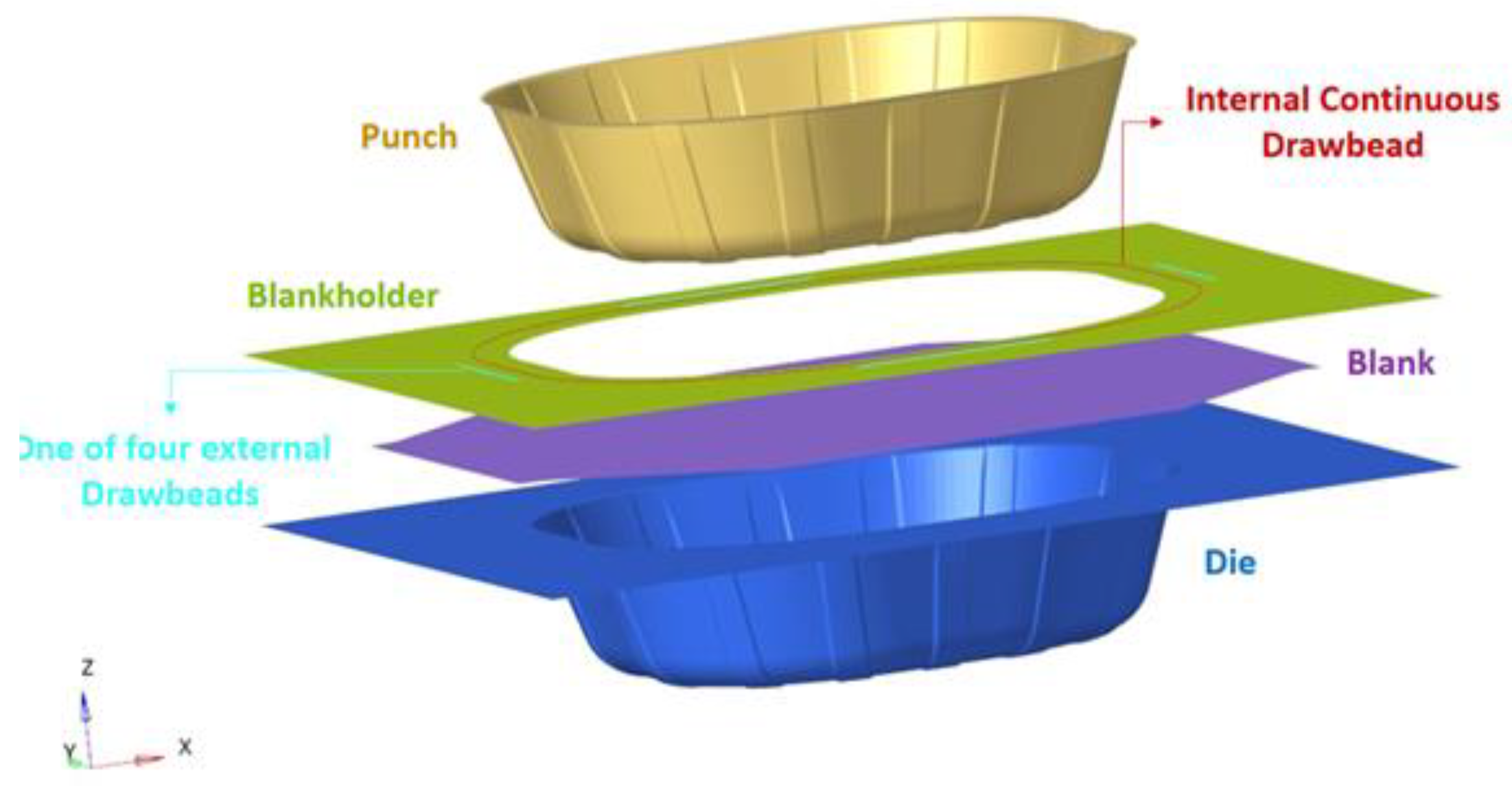
Figure 1.
Finite element (FE) model created for simulation of the sheet forming process.
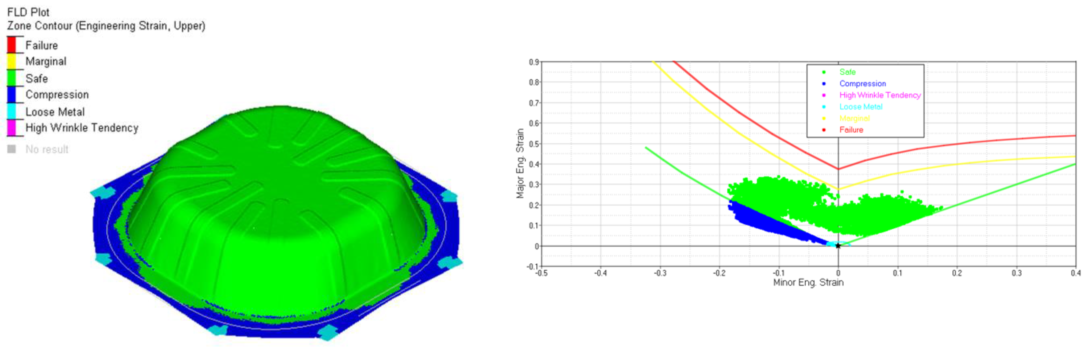
Figure 3.
Forming limit diagram (FLD) for RUN0.
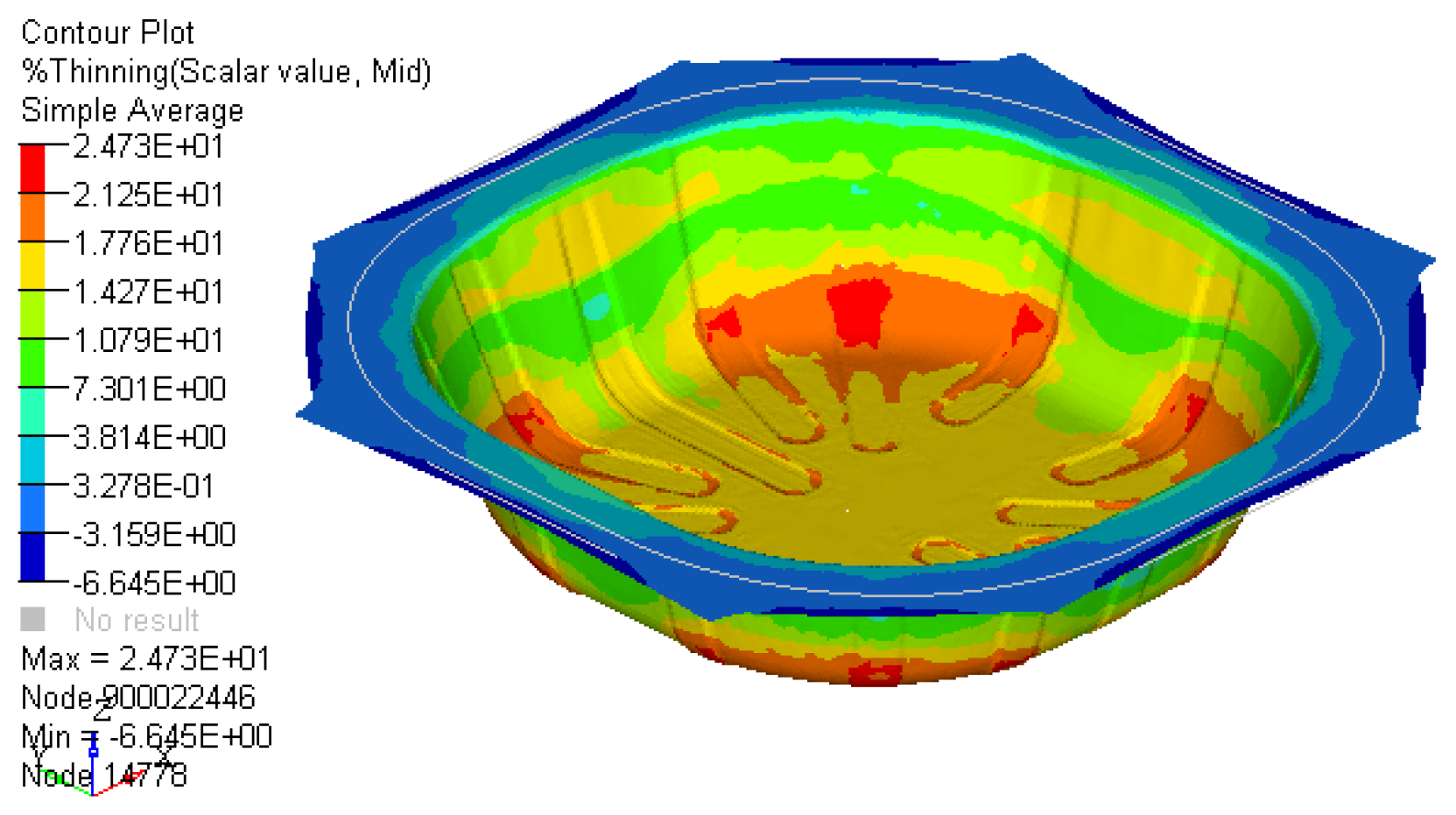
Figure 4.
% Thinning distribution for RUN0.
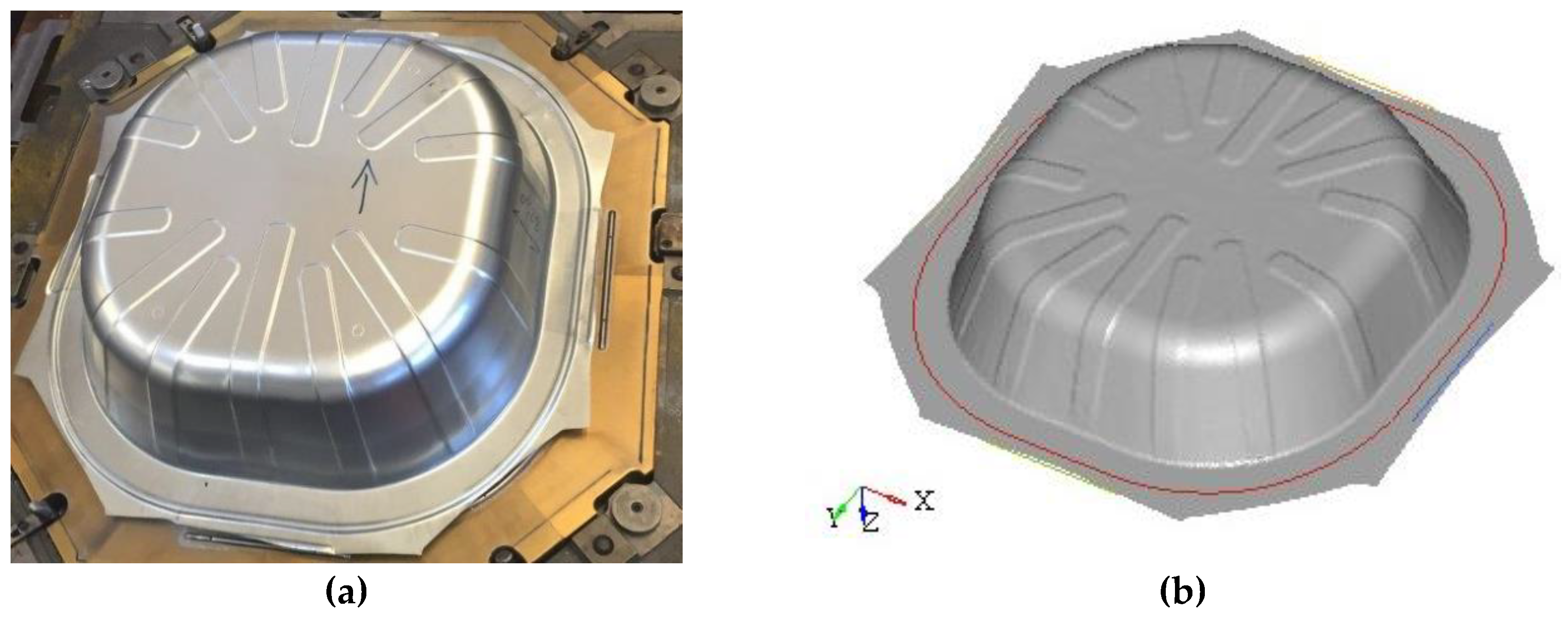
Figure 5.
Comparison between: (a) the real product obtained by forming using a traditional mechanical press and (b) the numerical model.
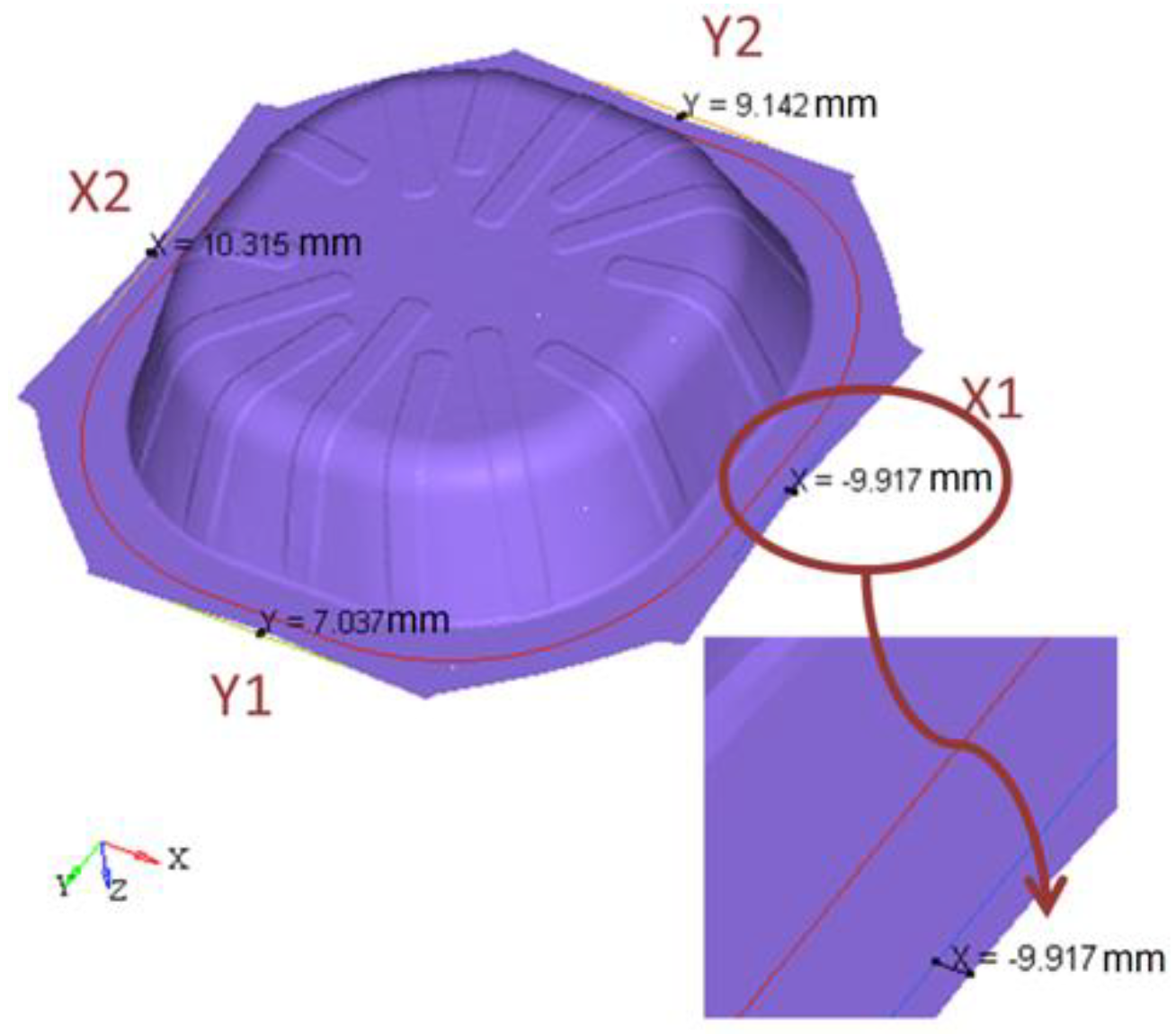
Figure 6.
Definition of output variables: X1, X2, Y1 and Y2 and related detail of X1.
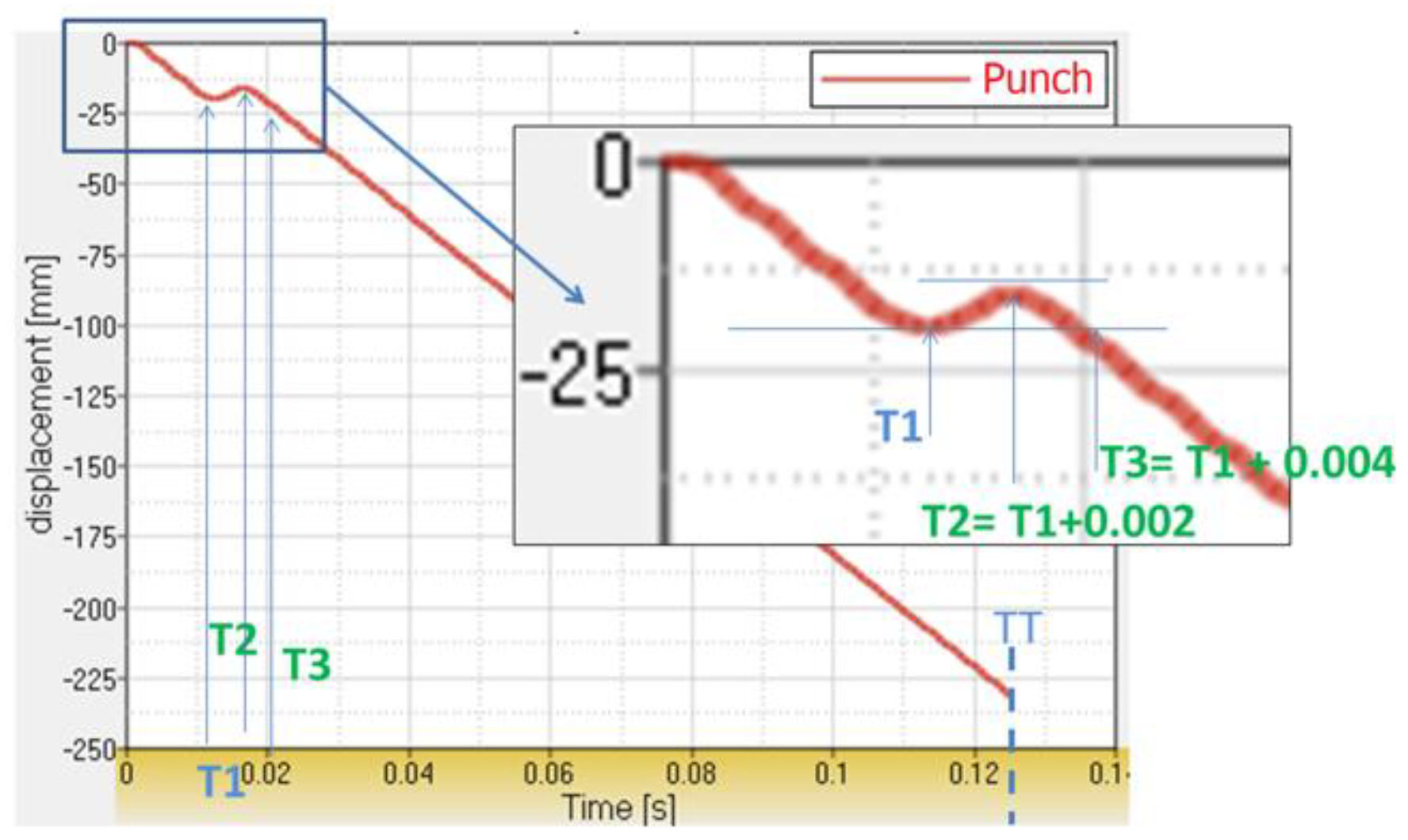
Figure 7.
Input timing definition on stepwise curve.
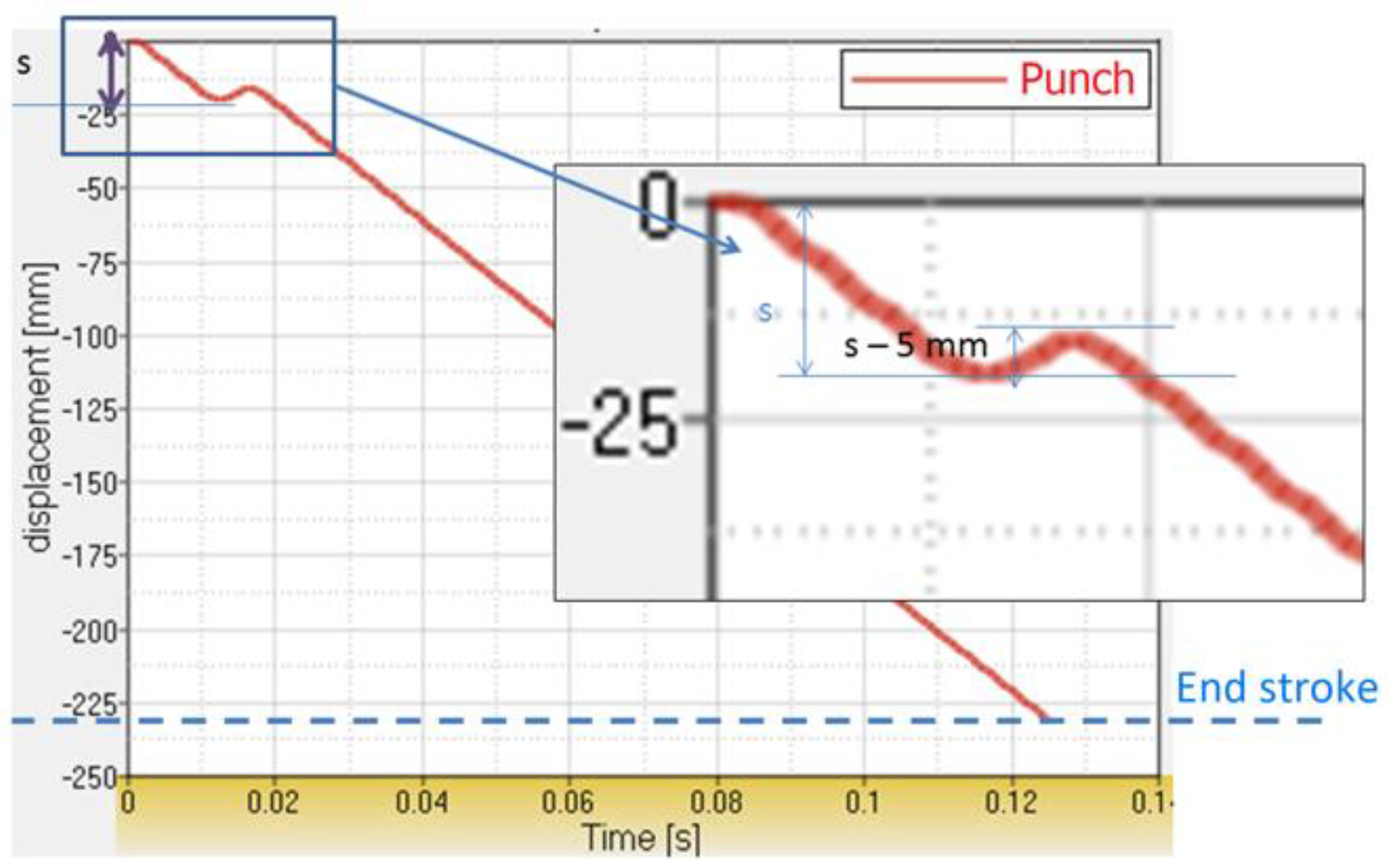
Figure 8.
Input stroke definition on stepwise curve.
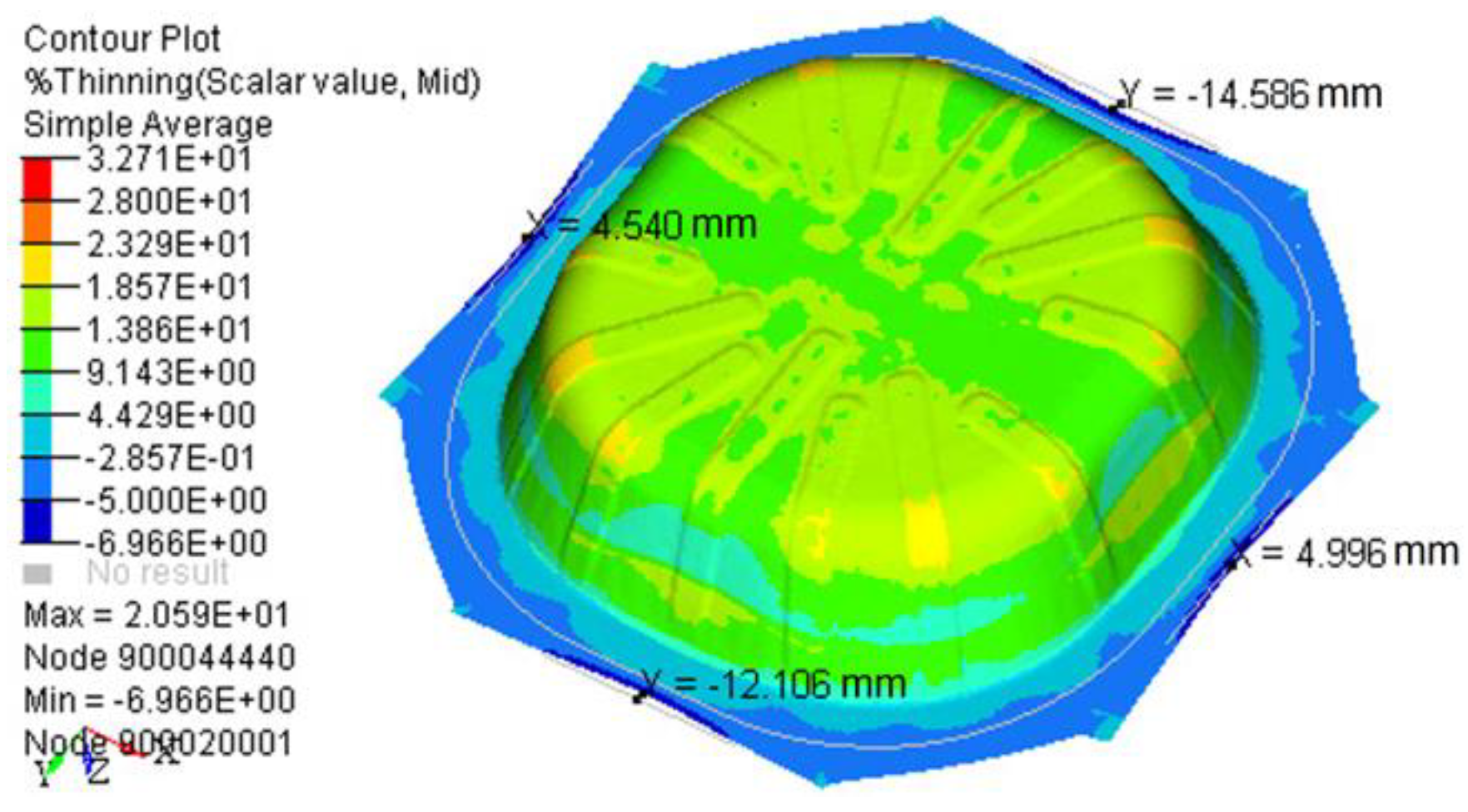
Figure 9.
% Thinning distribution and X1, X2, Y1 and Y2 values for the RUN22; blank0.
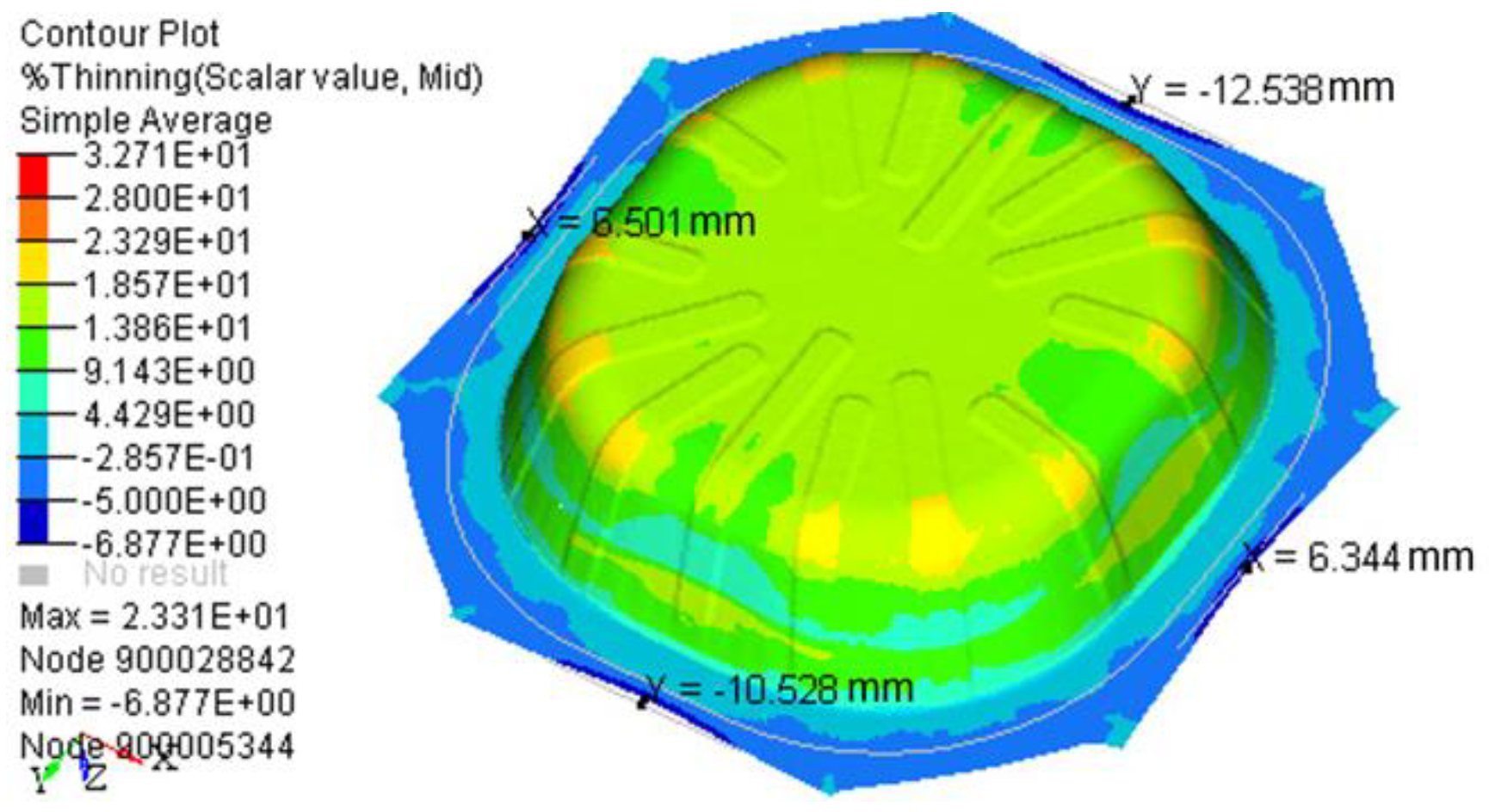
Figure 10.
% Thinning distribution and X1, X2, Y1 and Y2 values for the RUN20; blank0.
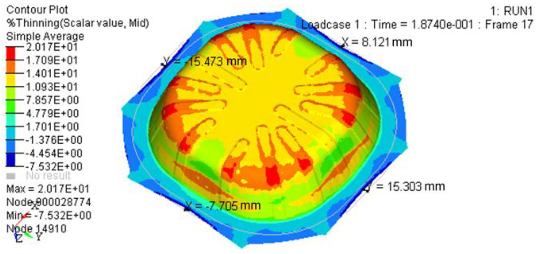
Figure 11.
% Thinning distribution and X1, X2, Y1 and Y2 values for the RUN1; blank1.
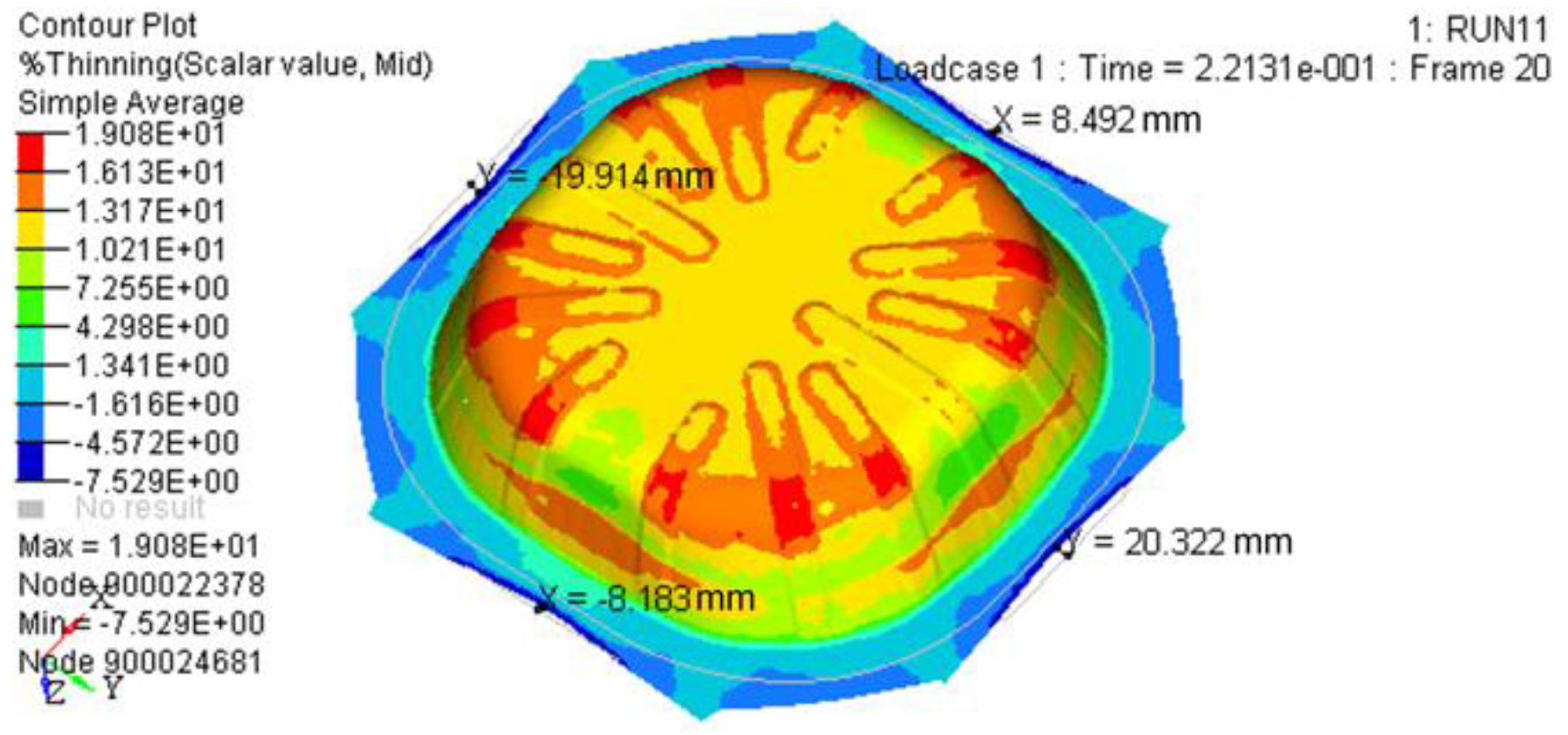
Figure 12.
% Thinning distribution and X1, X2, Y1 and Y2 values for the RUN11; blank1.
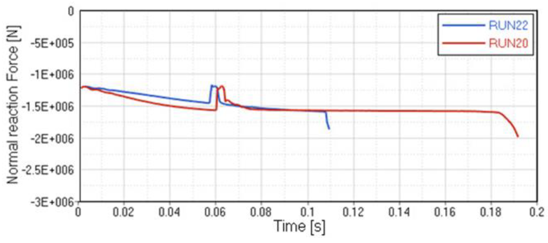
Figure 13.
Reaction force curves comparison between RUN20 and RUN22; blank0.
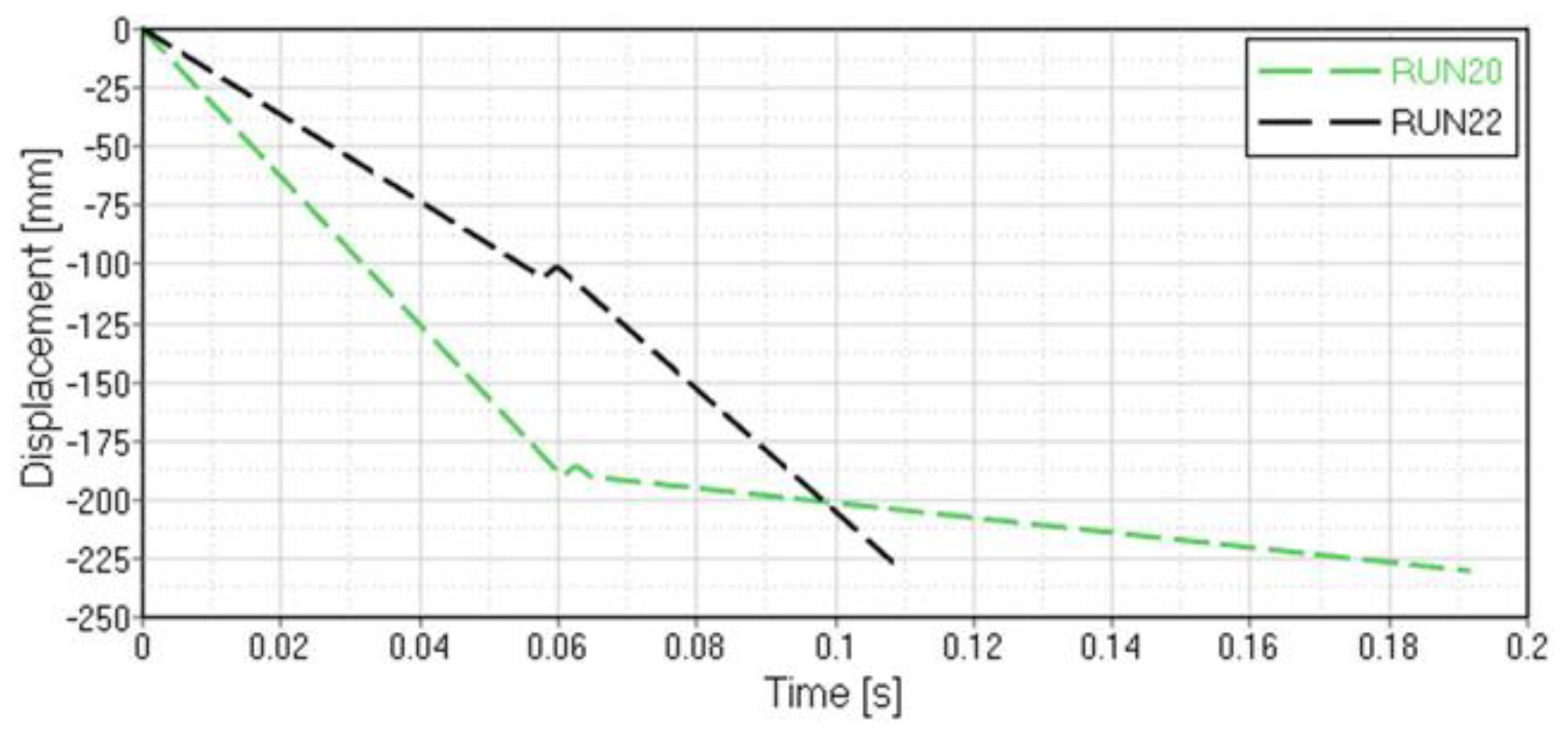
Figure 14.
Punch displacement with stepwise, in correspondence of S and T1. TT represents the last point of the curve with maximum value in the x axis; blank0.
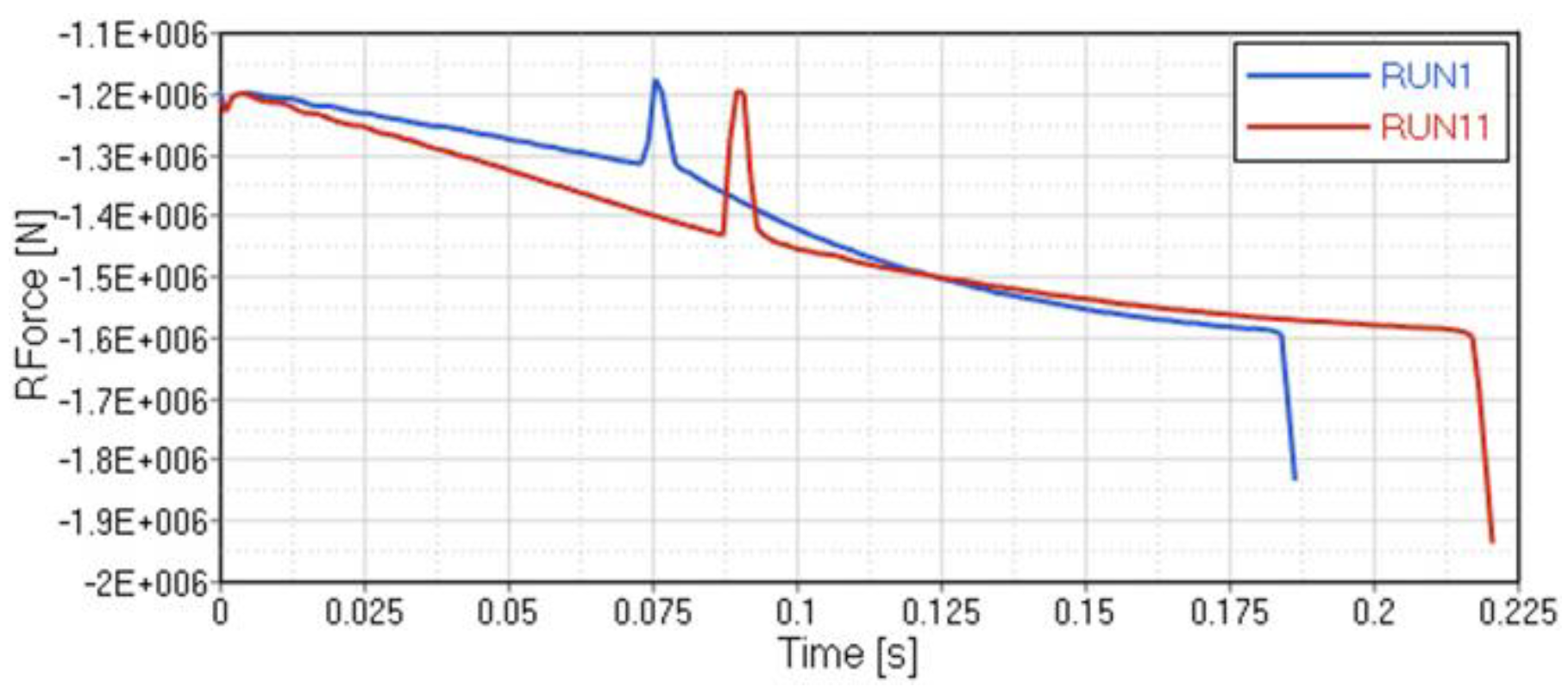
Figure 15.
Reaction force curves comparison between RUN1 and RUN11; blank1.
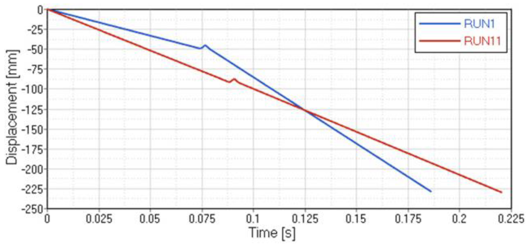
Figure 16.
Punch displacement with stepwise, in correspondence of S and T1. TT represents the last point of the curve with maximum value in x axis; blank1.
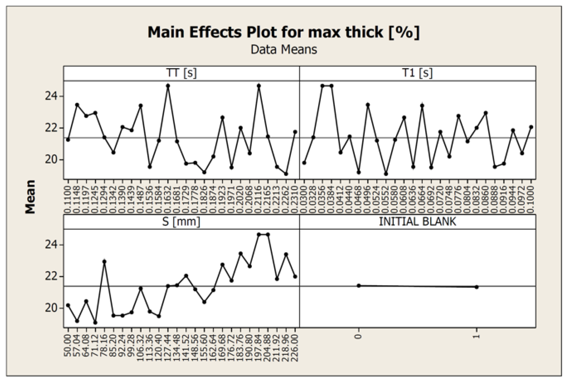
Figure 17.
MEP for max thick % output.
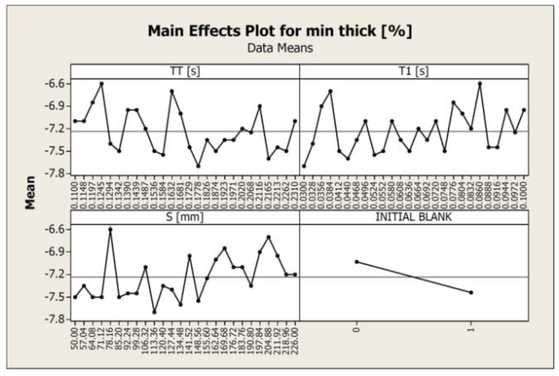
Figure 18.
MEP for min thick % output.
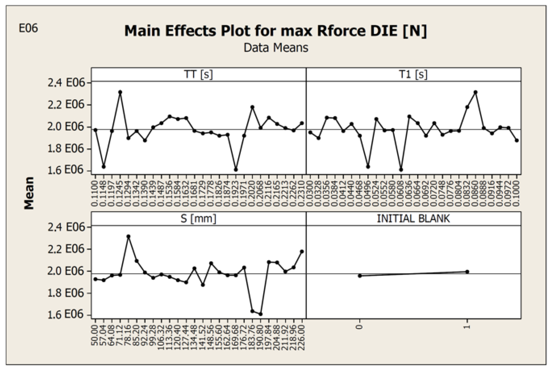
Figure 19.
MEP for reaction force output.
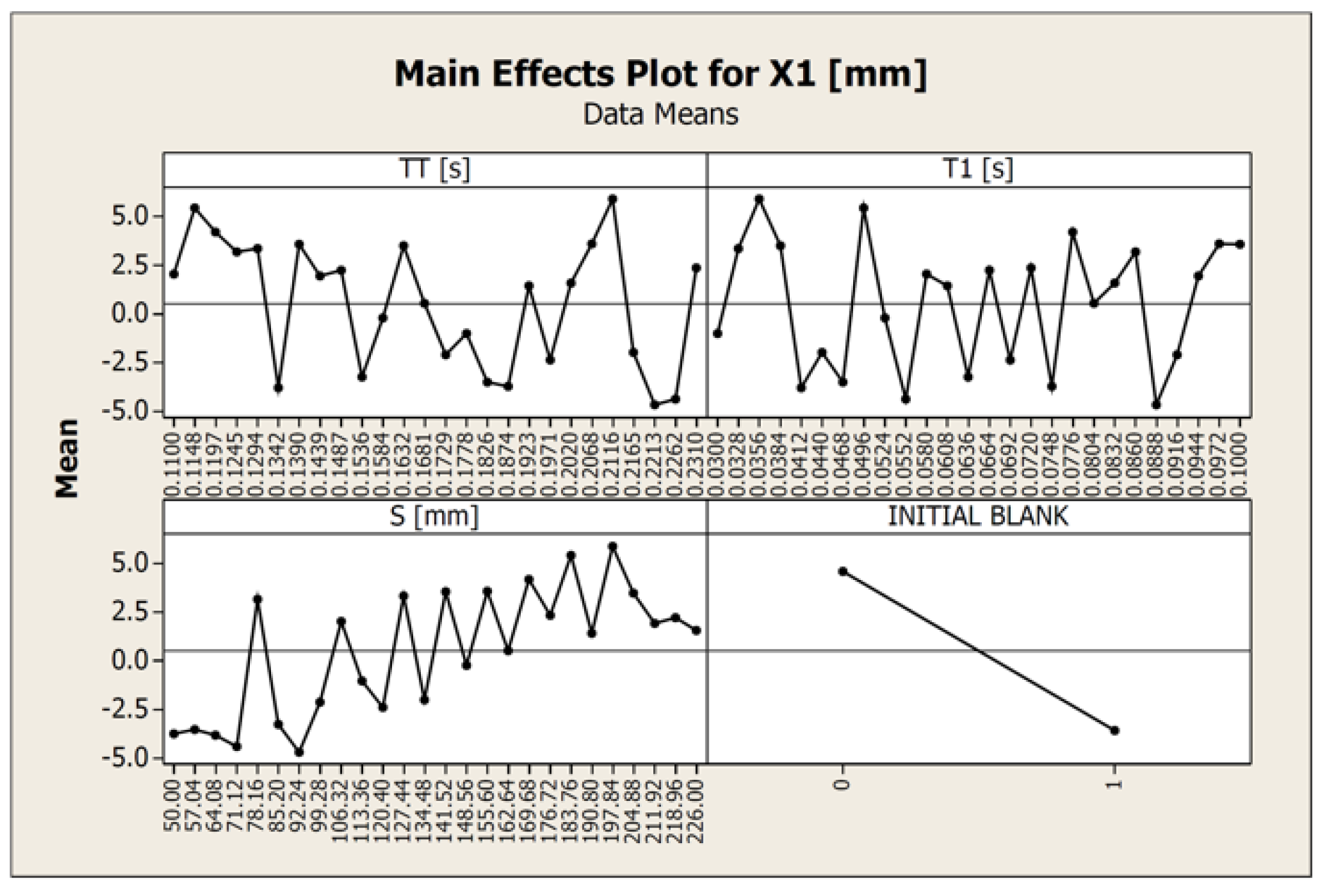
Figure 20.
MEP for X1 output.
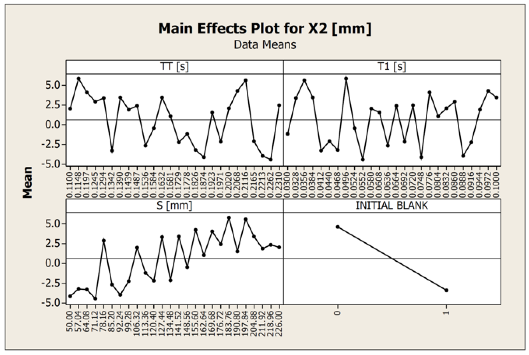
Figure 21.
MEP for X2 output.
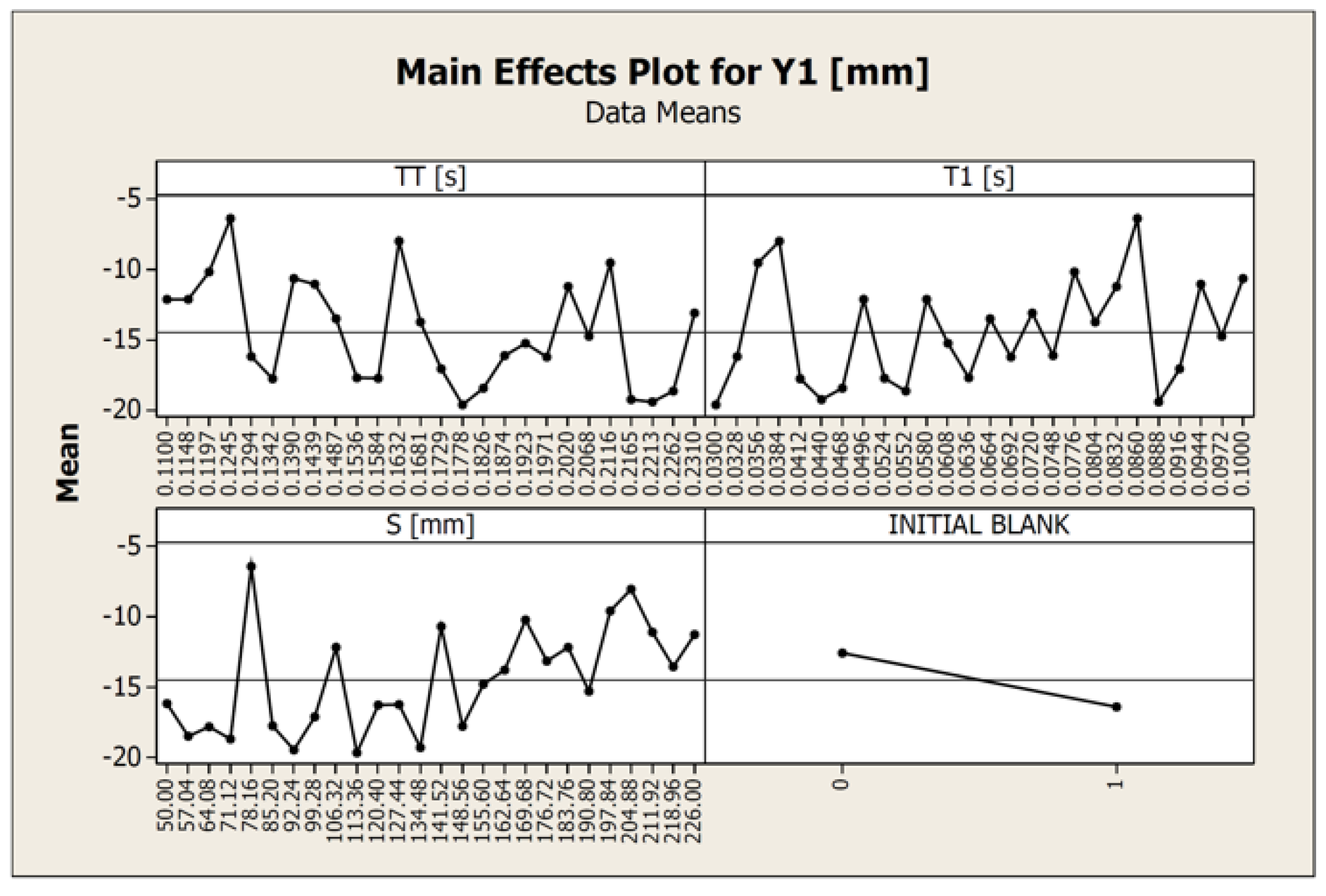
Figure 22.
MEP for Y1 output.
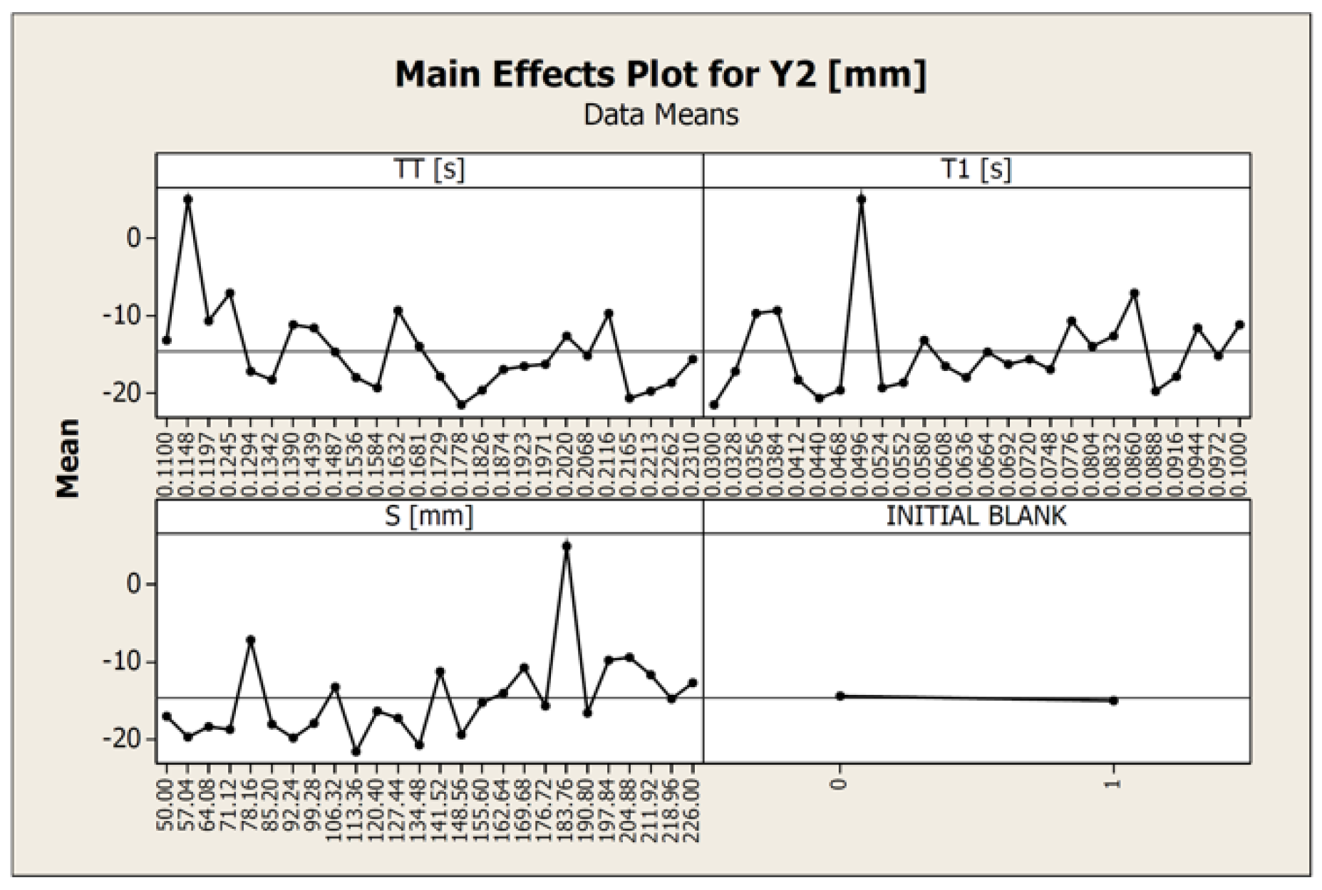
Figure 23.
MEP for Y2 output.
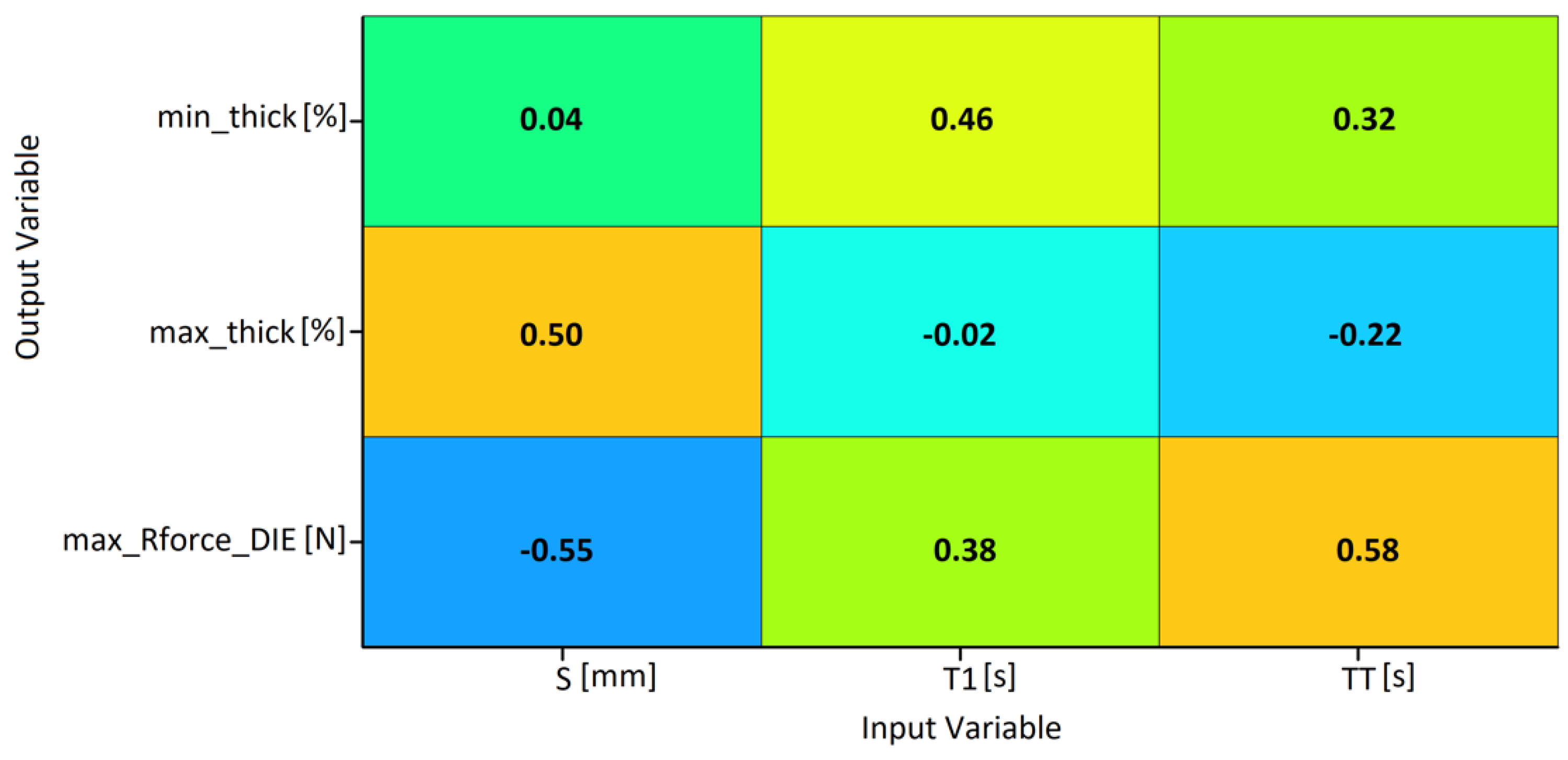
Figure 24.
Linear correlation matrix for the blank0 plan.
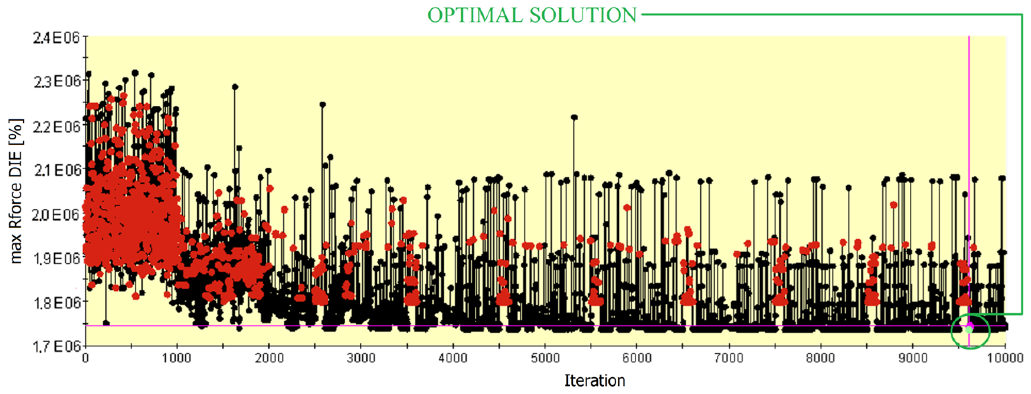
Figure 25.
Design explored with multi-island genetic algorithm (MIGA), blank0 plan.
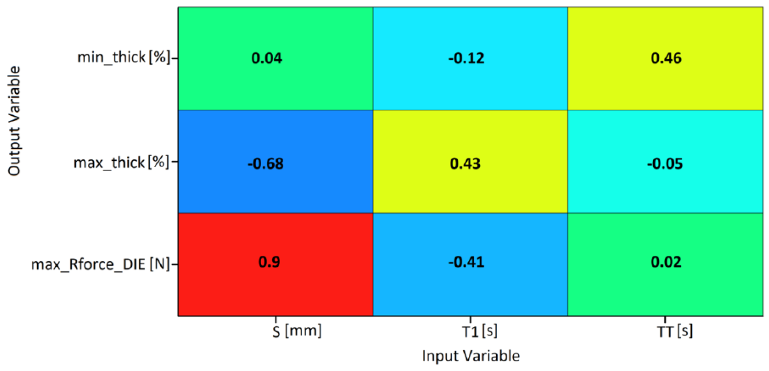
Figure 26.
Linear correlation matrix, blank 0.
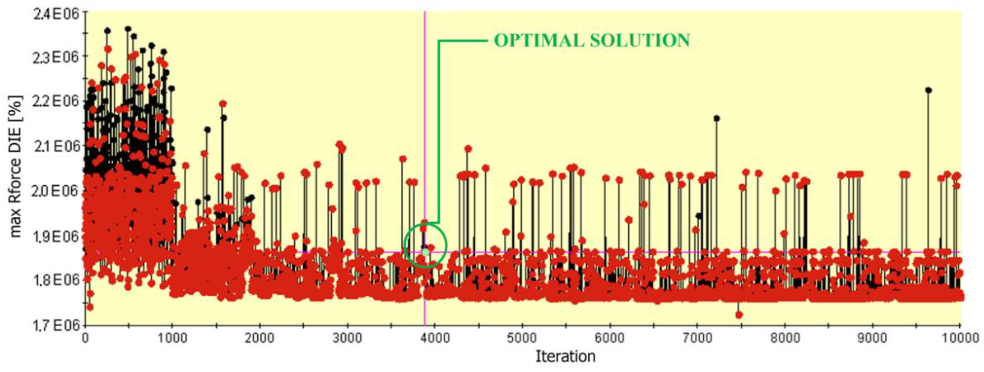
Figure 27.
Design explored with MIGA for the blank1 plan.
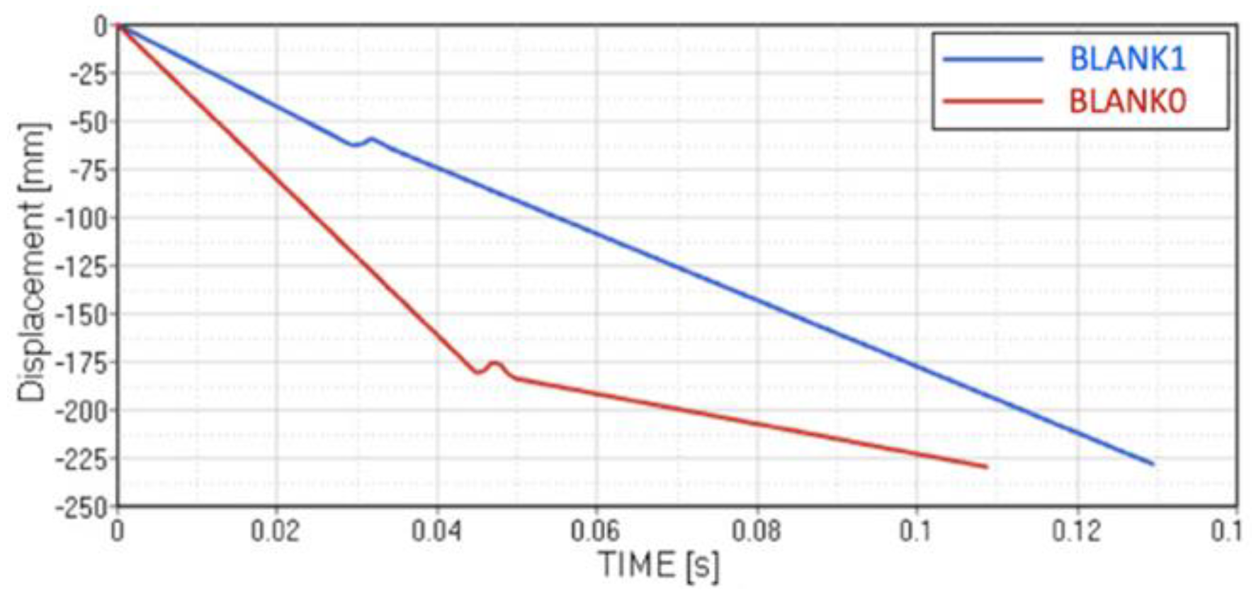
Figure 28.
Displacement vs time comparison for the optimal combination (according to the regression model) for blank0 and blank1 plan.
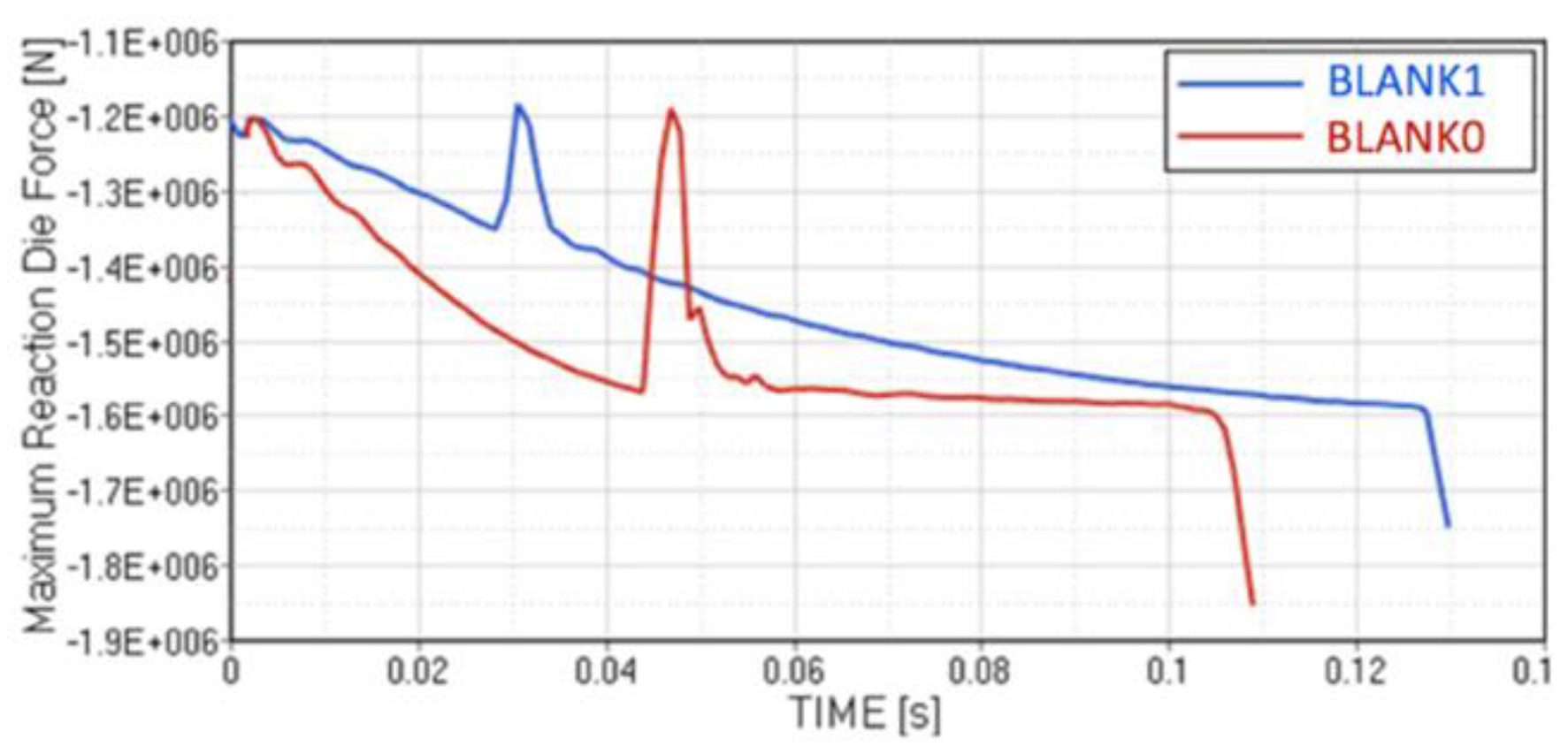
Figure 29.
Die reaction force comparison for both simulation plans.
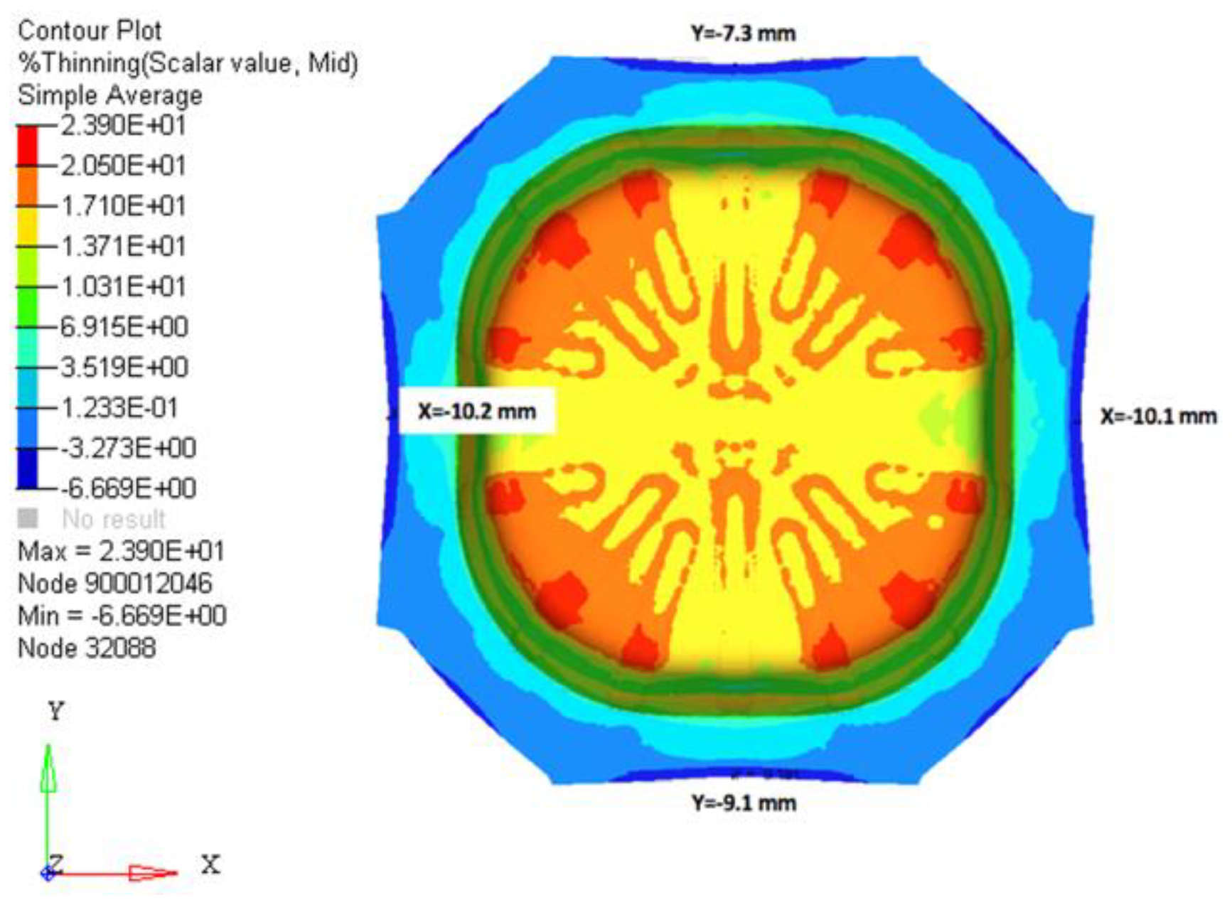
Figure 30.
%Thinning distribution and X1, X2, Y1 and Y2 for optimal combination for blank0.
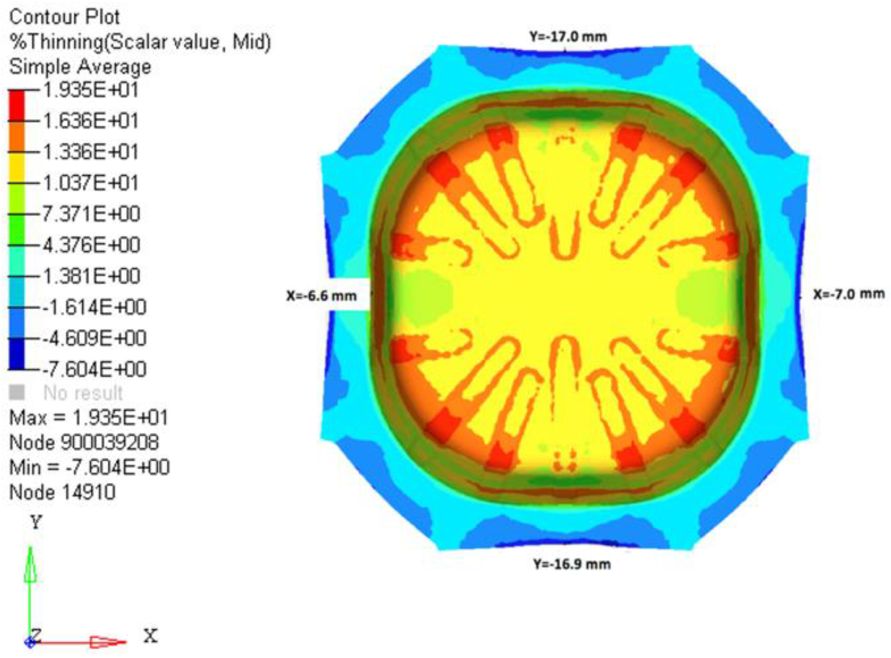
Figure 31.
%Thinning distribution and X1, X2, Y1 and Y2 for optimal combination for blank1.
Table 1.
DC04 (low-carbon steel) material properties and friction coefficient used in the simulation.
| σy (MPa) | Rm (MPa) | ν | h | B0 (MPa) | C | m | B (MPa) | Rsat (MPa) | n | μ |
|---|
| 130 | 500 | 0.3 | 0.526 | 168 | 657.9 | 1.281 | 8.980 | 558.6 | 0.19 | 0.125 |
Table 2.
Output variables list.
| Max Thickness (%) | Min Thickness (%) | Max Rforce DIE (N) | X1 (mm) | X2 (mm) | Y1 (mm) | Y2 (mm) |
|---|
| Output 1 | Output 2 | Output 3 | Output 4 | Output 5 | Output 6 | Output 7 |
Table 3.
Design variables for experiment plan runs.
| Run# | S (mm) | T1 (s) | TT (s) | Run# | S (mm) | T1 (s) | TT (s) |
|---|
| 1 | 50 | 0.0748 | 0.1874 | 14 | 162.64 | 0.0804 | 0.1681 |
| 2 | 99.28 | 0.0916 | 0.1729 | 15 | 155.6 | 0.0972 | 0.2068 |
| 3 | 211.92 | 0.0944 | 0.1439 | 16 | 183.76 | 0.0496 | 0.1148 |
| 4 | 57.04 | 0.0468 | 0.1826 | 17 | 141.52 | 0.1 | 0.139 |
| 5 | 226 | 0.0832 | 0.202 | 18 | 85.2 | 0.0636 | 0.1536 |
| 6 | 134.48 | 0.044 | 0.2165 | 19 | 64.08 | 0.0412 | 0.1342 |
| 7 | 197.84 | 0.0356 | 0.2116 | 20 | 190.8 | 0.0608 | 0.1923 |
| 8 | 78.16 | 0.086 | 0.1245 | 21 | 169.68 | 0.0776 | 0.1197 |
| 9 | 204.88 | 0.0384 | 0.1632 | 22 | 106.32 | 0.058 | 0.11 |
| 10 | 218.96 | 0.0664 | 0.1487 | 23 | 127.44 | 0.0328 | 0.1294 |
| 11 | 92.24 | 0.0888 | 0.2213 | 24 | 148.56 | 0.0524 | 0.1584 |
| 12 | 176.72 | 0.072 | 0.231 | 25 | 71.12 | 0.0552 | 0.2262 |
| 13 | 120.4 | 0.0692 | 0.1971 | 26 | 113.36 | 0.03 | 0.1778 |
Table 4.
Output of BLANK 0 simulation plan.
| Run | Max Thickness (%) | Min Thickness (%) | Max Rforce DIE (N) | X1 (mm) | X2 (mm) | Y1 (mm) | Y2 (mm) |
|---|
| 1 | 20.2 | −7.5 | 2.02 × 10⁶ | 0.632 | −0.517 | −16.984 | −18.473 |
| 2 | 20.0 | −7.3 | 1.92 × 10⁶ | 0.508 | −0.048 | −16.191 | −18.851 |
| 3 | 22.1 | −6.9 | 2.01 × 10⁶ | 5.97 | 5.691 | −10.963 | −12.754 |
| 4 | 19.3 | −7.4 | 1.97 × 10⁶ | −0.996 | −0.523 | −17.991 | −19.98 |
| 5 | 22.1 | −7.1 | 1.99 × 10⁶ | 5.058 | 5.365 | −11.243 | −13.195 |
| 6 | 21.0 | −7 | 2.01 × 10⁶ | 3.536 | 3.576 | −13.534 | −15.507 |
| 7 | 25.3 | −6.3 | 2.00 × 10⁶ | 14.672 | 14.819 | −3.418 | −5.069 |
| 8 | 23.1 | −6.6 | 2.76 × 10⁶ | 9.776 | 9.201 | −8.404 | −10.098 |
| 9 | 25.0 | −6.2 | 1.98 × 10⁶ | 14.01 | 14.455 | −3.736 | −5.168 |
| 10 | 22.6 | −6.7 | 2.01 × 10⁶ | 6.975 | 7.556 | −9.517 | −11.036 |
| 11 | 20 | −7.4 | 2.04 × 10⁶ | −0.839 | 0.209 | −18.533 | −19.615 |
| 12 | 21.6 | −7 | 2.02 × 10⁶ | 4.415 | 4.591 | −12.61 | −14.069 |
| 13 | 19.6 | −7.3 | 1.98 × 10⁶ | 1.049 | 1.192 | −15.7 | −17.665 |
| 14 | 21.1 | −7 | 1.93 × 10⁶ | 3.787 | 3.828 | −13.306 | −15.226 |
| 15 | 20.7 | −7.2 | 1.89 × 10⁶ | 3.298 | 3.819 | −13.848 | −15.51 |
| 16 | 23.5 | −6.7 | 1.20 × 10⁶ | 10.651 | 10.94 | −6.804 | −8.568 |
| 17 | 21.8 | −6.9 | 2.00 × 10⁶ | 6.657 | 6.285 | −10.66 | −12.524 |
| 18 | 19.3 | −7.4 | 2.13 × 10⁶ | −0.483 | 0.4 | −16.86 | −18.779 |
| 19 | 19.7 | −7.4 | 2.10 × 10⁶ | −0.513 | 0.362 | −16.986 | −19.325 |
| 20 | 23.3 | −6.9 | 1.20 × 10⁶ | 6.344 | 6.501 | −10.528 | −12.538 |
| 21 | 22.8 | −6.9 | 1.98 × 10⁶ | 7.009 | 6.67 | −10.403 | −11.965 |
| 22 | 20.6 | −7 | 1.87 × 10⁶ | 4.996 | 4.54 | −12.106 | −14.586 |
| 23 | 21.6 | −7 | 1.89 × 10⁶ | 5.988 | 5.698 | −11.908 | −13.041 |
| 24 | 21.5 | −7 | 2.05 × 10⁶ | 5.272 | 4.765 | −12.078 | −13.765 |
| 25 | 19.1 | −7.4 | −2.02 × 10⁶ | −0.675 | −0.919 | −17.808 | −19.328 |
| 26 | 20.3 | −7.3 | 1.95 × 10⁶ | 2.953 | 2.545 | −14.286 | −16.651 |
Table 5.
Output of BLANK 1 simulation plan.
| Run | Max Thickness (%) | Min Thickness (%) | Max Rforce DIE (N) | X1 (mm) | X2 (mm) | Y1 (mm) | Y2 (mm) |
|---|
| 1 | 20.2 | −7.5 | 1.84 × 10⁶ | −8.1 | −7.7 | −15.3 | −15.5 |
| 2 | 19.5 | −7.6 | 1.96 × 10⁶ | −4.7 | −4.4 | −18 | −16.9 |
| 3 | 21.6 | −7 | 1.98 × 10⁶ | −2.1 | −1.9 | −11.2 | −10.5 |
| 4 | 19.1 | −7.3 | 1.87 × 10⁶ | −6 | −5.9 | −18.9 | −19.3 |
| 5 | 21.9 | −7.3 | 2.37 × 10⁶ | −1.9 | −1.2 | −11.2 | −12.1 |
| 6 | 21.9 | −8.2 | 2.05 × 10⁶ | −7.5 | −7.8 | −25 | −25.8 |
| 7 | 24 | −7.5 | 2.17 × 10⁶ | −2.9 | −3.6 | −15.7 | −14.4 |
| 8 | 22.8 | −6.6 | 1.88 × 10⁶ | −3.4 | −3.4 | −4.4 | −4.1 |
| 9 | 24.3 | −7.2 | 2.18 × 10⁶ | −7 | −7.6 | −12.3 | −13.6 |
| 10 | 24.2 | −7.7 | 2.06 × 10⁶ | −2.5 | −2.8 | −17.5 | −18.4 |
| 11 | 19.1 | −7.5 | 1.94 × 10⁶ | −8.5 | −8.2 | −20.3 | −19.9 |
| 12 | 21.9 | −7.2 | 2.04 × 10⁶ | 0.3 | 0.3 | −13.6 | −17.2 |
| 13 | 19.4 | −7.4 | 1.86 × 10⁶ | −5.8 | −5.5 | −16.8 | −14.9 |
| 14 | 21.2 | −7 | 2.00 × 10⁶ | −2.7 | −1.7 | −14.2 | −12.8 |
| 15 | 20.1 | −7.3 | 2.09 × 10⁶ | 3.9 | 4.7 | −15.7 | −14.9 |
| 16 | 23.4 | −7.5 | 2.08 × 10⁶ | 0.2 | 0.7 | −17.5 | 18.5 |
| 17 | 22.3 | −7 | 1.75 × 10⁶ | 0.5 | 0.6 | −10.7 | −9.9 |
| 18 | 19.8 | −7.6 | 2.06 × 10⁶ | −6 | −5.7 | −18.6 | −17.2 |
| 19 | 21.2 | −7.6 | 1.82 × 10⁶ | −7.1 | −6.9 | −18.6 | −17.3 |
| 20 | 22 | −7.8 | 2.02 × 10⁶ | −3.5 | −3.4 | −20 | −20.6 |
| 21 | 22.7 | −6.8 | 1.95 × 10⁶ | 1.4 | 1.5 | −10 | −9.5 |
| 22 | 21.9 | −7.2 | 2.07 × 10⁶ | −0.9 | −0.5 | −12.2 | −11.8 |
| 23 | 21.2 | −7.8 | 1.91 × 10⁶ | 0.7 | 1 | −20.5 | −21.4 |
| 24 | 20.9 | −8.1 | 2.10 × 10⁶ | −5.7 | −5.7 | −23.4 | −24.9 |
| 25 | 19.1 | −7.6 | 1.91 × 10⁶ | −8.1 | −7.9 | −19.5 | −18 |
| 26 | 19.3 | −8.1 | 1.95 × 10⁶ | −5 | −4.9 | −25 | −26.4 |
Table 6.
Numerical and regression model values correlation for the blank0 plan.
| Run | Input | Regression Model Outputs | Numerical Outputs | Errors |
|---|
| S (mm) | T1 (s) | TT (s) | Max Thick (%) | Min Thick (%) | Max Rforce DIE (N) | Max Thick (%) | Min Thick (%) | Max Rforce DIE (N) | Max Thick (%) | Min Thick (%) | Max Rforce DIE (N) |
|---|
| 1 | 50.00 | 0.0748 | 0.1874 | 20.02 | −7.34 | 2093295 | 20.20 | −7.50 | 2022870 | −0.91 | −2.10 | 3.48 |
| 2 | 99.28 | 0.0916 | 0.1729 | 20.78 | −7.17 | 2182846 | 20.00 | −7.30 | 1918110 | 3.92 | −1.83 | 13.80 |
| 3 | 211.92 | 0.0944 | 0.1439 | 22.11 | −6.92 | 1993481 | 22.10 | −6.90 | 2013660 | 0.04 | 0.30 | −1.00 |
| 4 | 57.04 | 0.0468 | 0.1826 | 18.80 | −7.58 | 1892017 | 19.30 | −7.40 | 1968800 | −2.60 | 2.48 | −3.90 |
| 5 | 226.00 | 0.0832 | 0.2020 | 22.40 | −6.99 | 2063007 | 22.10 | −7.10 | 1989740 | 1.35 | −1.57 | 3.68 |
| 6 | 134.48 | 0.0440 | 0.2165 | 21.22 | −7.05 | 1897945 | 21.00 | −7.00 | 2008330 | 1.05 | 0.65 | −5.50 |
| 7 | 197.84 | 0.0356 | 0.2116 | 25.47 | −6.19 | 2109164 | 25.30 | −6.30 | 1999097 | 0.65 | −1.76 | 5.51 |
| 8 | 78.16 | 0.0860 | 0.1245 | 22.47 | −6.78 | 2547603 | 23.10 | −6.60 | 2755880 | 0.31 | 1.22 | −6.73 |
| 9 | 204.88 | 0.0384 | 0.1632 | 24.86 | −6.29 | 1936617 | 25.00 | −6.20 | 1982690 | −0.55 | 1.41 | −2.32 |
| 10 | 218.96 | 0.0664 | 0.1487 | 23.37 | −6.65 | 2011086 | 22.60 | −6.70 | 2008650 | 3.43 | −0.68 | 0.12 |
| 11 | 92.24 | 0.0888 | 0.2213 | 20.00 | −7.29 | 2081651 | 20.00 | −7.40 | 2039430 | 0.00 | −1.43 | 2.07 |
| 12 | 176.72 | 0.0720 | 0.2310 | 21.56 | −7.07 | 2061384 | 21.60 | −7.00 | 2023390 | −0.17 | 0.94 | 1.88 |
| 13 | 120.40 | 0.0692 | 0.1971 | 19.88 | −7.37 | 1888758 | 19.60 | −7.30 | 1981650 | 1.44 | 0.99 | −4.69 |
| 14 | 162.64 | 0.0804 | 0.1681 | 20.83 | −7.20 | 1915638 | 21.10 | −7.00 | 1927210 | −1.27 | 2.79 | −0.60 |
| 15 | 155.60 | 0.0972 | 0.2068 | 20.32 | −7.31 | 1696835 | 20.70 | −7.20 | 1893290 | −1.85 | 1.51 | −10.38 |
| 16 | 183.76 | 0.0496 | 0.1148 | 23.38 | −6.51 | 1556814 | 23.50 | −6.70 | 1200260 | 4.85 | −5.71 | −17.74 |
| 17 | 141.52 | 0.1000 | 0.1390 | 21.95 | −6.89 | 2071463 | 21.80 | −6.90 | 2001060 | 0.70 | −0.20 | 3.52 |
| 18 | 85.20 | 0.0636 | 0.1536 | 20.00 | −7.34 | 2177074 | 19.30 | −7.40 | 2130240 | 3.60 | −0.81 | 2.20 |
| 19 | 64.08 | 0.0412 | 0.1342 | 19.57 | −7.41 | 2086636 | 19.70 | −7.40 | 2100820 | −0.67 | 0.16 | −0.68 |
| 20 | 190.80 | 0.0608 | 0.1923 | 22.36 | −6.90 | 1770676 | 23.30 | −6.90 | 1200110 | 0.29 | 0.02 | −11.90 |
| 21 | 169.68 | 0.0776 | 0.1197 | 22.20 | −6.81 | 1906247 | 22.80 | −6.90 | 1977980 | −2.62 | −1.34 | −3.63 |
| 22 | 106.32 | 0.0580 | 0.1100 | 21.37 | −6.97 | 1899818 | 20.60 | −7.00 | 1873870 | 3.74 | −0.39 | 1.38 |
| 23 | 127.44 | 0.0328 | 0.1294 | 21.40 | −6.94 | 1947060 | 21.60 | −7.00 | 1889500 | −0.93 | −0.84 | 3.05 |
| 24 | 148.56 | 0.0524 | 0.1584 | 21.15 | −7.08 | 1807338 | 21.50 | −7.00 | 2045660 | −1.63 | 1.15 | −11.65 |
| 25 | 71.12 | 0.0552 | 0.2262 | 19.18 | −7.44 | 2027902 | 19.10 | −7.40 | 2024410 | 0.39 | 0.59 | 0.17 |
| 26 | 113.36 | 0.0300 | 0.1778 | 20.59 | −7.15 | 2059791 | 20.30 | −7.30 | 1952500 | 1.45 | −2.04 | 5.50 |
| Min | 50.00 | 0.030 | 0.11 | 18.80 | −7.58 | 1556814 | 19.10 | −7.50 | 1200110 | −2.62 | −5.71 | −17.74 |
| Max | 226.00 | 0.10 | 0.23 | 25.47 | −6.19 | 2547603 | 25.30 | −6.20 | 2755880 | 4.85 | 2.79 | 13.80 |
Table 7.
Optimal combination of regression model; Blank0.
| S (mm) | T1 (s) | TT (s) | Max Rforce DIE (N) | Max Thick (%) | Min Thick (%) | Objective and Penalty | Objective Function (N) | Penalty Function |
|---|
| 182.847974 | 0.0454548 | 0.11000185 | 1472516 | 20 | −6.42 | 1472516 | 1472516 | 0 |
Table 8.
Numerical and regression model values correlation for blank1 plan.
| Run | Input | Regression Model Outputs | Numerical Outputs | Errors |
|---|
| S (mm) | T1 (s) | TT (s) | Max Thick (%) | Min Thick (%) | S (mm) | T1 (s) | TT (s) | Max Thick (%) | Max Thick (%) | S (mm) | T1 (s) |
|---|
| 1 | 50.00 | 0.0748 | 0.1874 | 19.80 | −7.42 | 1834375.021 | 20.20 | −7.50 | 1835260 | −1.96 | −1.07 | −0.05 |
| 2 | 99.28 | 0.0916 | 0.1729 | 20.12 | −7.49 | 1937125.107 | 19.50 | −7.60 | 1964070 | 3.17 | −1.51 | −1.37 |
| 3 | 211.92 | 0.0944 | 0.1439 | 22.17 | −7.02 | 1972896.543 | 21.60 | −7.00 | 1981810 | 2.66 | 0.23 | −0.45 |
| 4 | 57.04 | 0.0468 | 0.1826 | 19.05 | −7.58 | 1867188.059 | 19.10 | −7.30 | 1871000 | −0.25 | 3.82 | −0.20 |
| 5 | 226.00 | 0.0832 | 0.2020 | 22.41 | −7.27 | 2311269.029 | 21.90 | −7.30 | 2371100 | 2.32 | −0.47 | −2.52 |
| 6 | 134.48 | 0.0440 | 0.2165 | 20.84 | −7.61 | 2019189.077 | 21.90 | −8.20 | 2045330 | −4.84 | −7.16 | −1.28 |
| 7 | 197.84 | 0.0356 | 0.2116 | 24.39 | −7.57 | 2158267.881 | 24.00 | −7.50 | 2168100 | 1.62 | 0.92 | −0.45 |
| 8 | 78.16 | 0.0860 | 0.1245 | 22.79 | −6.72 | 1880775.054 | 22.80 | −6.60 | 1877480 | −0.05 | 1.86 | 0.18 |
| 9 | 204.88 | 0.0384 | 0.1632 | 23.84 | −8.09 | 2138040.466 | 24.30 | −7.20 | 2178410 | −1.91 | 12.37 | −1.85 |
| 10 | 218.96 | 0.0664 | 0.1487 | 23.37 | −7.60 | 2146448.837 | 24.20 | −7.70 | 2060450 | −3.41 | −1.26 | 4.17 |
| 11 | 92.24 | 0.0888 | 0.2213 | 19.26 | −7.45 | 1965398.706 | 19.10 | −7.50 | 1939120 | 0.83 | −0.60 | 1.36 |
| 12 | 176.72 | 0.0720 | 0.2310 | 21.55 | −7.28 | 2057738.866 | 21.90 | −7.20 | 2044910 | −1.61 | 1.05 | 0.63 |
| 13 | 120.40 | 0.0692 | 0.1971 | 19.69 | −7.71 | 2028697.012 | 19.40 | −7.40 | 1858140 | 1.47 | 4.17 | 9.18 |
| 14 | 162.64 | 0.0804 | 0.1681 | 20.66 | −7.56 | 1956293.479 | 21.20 | −7.00 | 2001820 | −2.52 | 7.94 | −2.27 |
| 15 | 155.60 | 0.0972 | 0.2068 | 19.58 | −7.31 | 2022827.292 | 20.10 | −7.30 | 2089730 | −2.59 | 0.19 | −3.20 |
| 16 | 183.76 | 0.0496 | 0.1148 | 23.54 | −7.52 | 2057717.659 | 23.40 | −7.50 | 2076100 | 0.62 | 0.32 | −0.89 |
| 17 | 141.52 | 0.1000 | 0.1390 | 21.55 | −6.69 | 1841041.399 | 22.30 | −7.00 | 1753830 | −3.38 | −0.62 | 4.97 |
| 18 | 85.20 | 0.0636 | 0.1536 | 20.29 | −7.66 | 1942531.283 | 19.80 | −7.60 | 2058790 | 2.50 | 0.78 | −5.65 |
| 19 | 64.08 | 0.0412 | 0.1342 | 20.31 | −7.48 | 1895316.719 | 21.20 | −7.60 | 1824710 | −4.18 | −1.62 | 3.87 |
| 20 | 190.80 | 0.0608 | 0.1923 | 22.08 | −7.70 | 2140322.430 | 22.00 | −7.80 | 2020780 | 0.38 | −1.34 | 5.92 |
| 21 | 169.68 | 0.0776 | 0.1197 | 22.72 | −6.94 | 1910920.430 | 22.70 | −6.80 | 1949350 | 0.09 | 2.11 | −1.97 |
| 22 | 106.32 | 0.0580 | 0.1100 | 22.36 | −6.99 | 2048391.365 | 21.90 | −7.20 | 2069810 | 2.11 | −2.91 | −1.03 |
| 23 | 127.44 | 0.0328 | 0.1294 | 21.23 | −8.02 | 1960883.548 | 21.20 | −7.80 | 1908440 | 0.12 | 2.85 | 2.75 |
| 24 | 148.56 | 0.0524 | 0.1584 | 20.99 | −7.96 | 1997574.579 | 20.90 | −8.10 | 2098800 | 0.45 | −1.78 | −4.82 |
| 25 | 71.12 | 0.0552 | 0.2262 | 19.27 | −7.45 | 1880469.975 | 19.10 | −7.60 | 1911420 | 0.88 | −1.97 | −1.62 |
| 26 | 113.36 | 0.0300 | 0.1778 | 19.96 | −7.91 | 1935405.070 | 19.30 | −8.10 | 1948510 | 3.40 | −2.32 | −0.67 |
| Min | 50.00 | 0.030 | 0.11 | 19.05 | −8.09 | 1834375.021 | 19.10 | −8.20 | 1753830 | −4.84 | −7.16 | −5.65 |
| Max | 226.00 | 0.10 | 0.23 | 24.39 | −6.69 | 2311269.029 | 24.30 | −6.60 | 2371100 | 3.40 | 12.37 | 9.18 |
Table 9.
Optimal combination of regression model for Blank1.
| S (mm) | T1 (s) | TT (s) | Max Rforce DIE (N) | Max Thick (%) | Min Thick (%) | Objective and Penalty | Objective Function (N) | Penalty Function |
|---|
| 64.23899 | 0.031864 | 0.131 | 1863534.957 | 20 | −7.43 | 1863534.957 | 1863534.957 | 0 |
Table 10.
Output for optimal models: blank0 (optimal0) and blank 1 (optimal1).
| Run | Max Thickness (%) | Min Thickness (%) | Max Rforce DIE (N) | X1 (mm) | X2 (mm) | Y1 (mm) | Y2 (mm) |
|---|
| Optimal0 | 23.9 | −6.7 | 1855 | −10.2 | −10.1 | −9.1 | −7.3 |
| Optimal1 | 19.3 | −7.6 | 1751 | −6.6 | −7.0 | −16.9 | −17.0 |
Table 11.
Percentage error calculation of numerical results vs regression model results.
| Run | Max Thick Error (%) | Min Thick Error (%) | Max Rforce DIE Error (kN) |
|---|
| Optimal0 | −19.5 | 4.4 | −26% |
| Optimal1 | 3.2 | 2.3 | 6.0% |


