History Reduction by Lumping for Time-Efficient Simulation of Additive Manufacturing

Abstract

Additive manufacturing is the process by which material is added layer by layer. In most cases, many layers are added, and the passes are lengthy relative to their thicknesses and widths. This makes finite element simulations of the process computationally demanding owing to the short time steps and large number of elements. The classical lumping approach in computational welding mechanics, popular in the 80s, is therefore, of renewed interest and is evaluated in this work. The method of lumping means that welds are merged. This allows fewer time steps and a coarser mesh. It was found that the computation time can be reduced considerably, with retained accuracy for the resulting temperatures and deformations. The residual stresses become, to a certain degree, smaller. The simulations were validated against a directed energy deposition (DED) experiment with alloy 625.

1. Introduction

Additive manufacturing (AM) is a process by which a product is built by adding the material layer by layer. This method provides new opportunities from the design and manufacturing points of view. It is possible to create complex shapes, which can be utilized for the design of optimized geometries with the possibility of saving weight. It can also be used to repair existing products. Other advantages are the reduced material waste and shorter component lead-time [1]. However, a challenge with AM is how to minimize the distortions and residual stresses of the final product.

The finite element method (FEM) can be used to predict the resulting distortion and residual stresses. This leads to additional knowledge about the process and may also reduce the number of trial and error experiments necessary to find the process parameters. There are a number of publications about simulation of additive manufacturing; e.g., [2,3,4,5,6].

Finite element simulations of the AM process are computationally demanding owing to the short time steps and large number of elements involved. This is one of the main reasons why simulation of AM is not widely used. Several approaches are aimed at reducing the computational effort. Umer et al. [7] make use of dimensional reduction in their thermo-mechanical model to study the effect of different support structures in electron beam melting. A 2D model is not suitable for all geometries, and it will always introduce a loss of details in the problem. Remeshing is a useful tool for spatial reduction. Remeshing has been performed layer by layer [8,9,10] and locally, near the heat source [11,12]. Moreover, different techniques for merging or lumping layers and passes have been used. Lumping is a history-reduction approach and was used in the early era of computational welding mechanics (CWM) for multipass welding, as can be seen in reviews [13,14]. In additive manufacturing, Chiumenti et al. [15] investigated the results of thermal simulations when the material was added hatch by hatch or layer by layer in the simulation. The simulation time was reduced by up to 98% and the average temperature history was captured, but not the local thermal history. Prabhakar et al. [16] used a thermo-mechanical model where whole layers were added simultaneously when a part with 50 layers was built. This model was validated against an experiment. Keller et al. [17,18] described a model where several layers were added simultaneously. With their model they were able to predict deformation and residual stresses at the macroscopic level. In the current work the temperature and deformation evolution is studied when the passes are added transiently, and only lumped in the build direction. To the authors’ knowledge there is no publication where the approach has been used in this way. The inherent strain method is another approach for fast prediction of the resulting deformation and residual stress in AM processes [19,20]. The method was first proposed for welding by Ueda and coworkers [21,22,23]. Li et al. [24,25] used the inherent strain approach, but instead of using strain, a residual stress tensor is added to each layer in the mechanical macro-scale model. The simulation was performed with a multi-scale model in three different scales. A micro-scale model was used to predict an equivalent heat source, which was the input to the meso-scale model. Because the AM process is very fast, it was assumed that the heat could be added to the whole layer simultaneously. In the thermo-mechanical meso-scale model, a residual stress tensor from one added layer was calculated. Finally, the mechanical model on the macro-scale was computed, wherein the material was added layer by layer and the pre-determined residual stress tensor was applied on each added layer. The drawback with the inherent strain method is that it often requires calibration. The inherent strains are in general sensitive to changes in the boundary conditions.

The main aim of this work was to study the method lumping of welds, described above, and evaluate the error introduced in the modeling and the achieved reduction in computation time for the simulations. A detailed thermo-mechanical FE model was validated with in situ temperature and displacement measurements for directed energy deposition (DED) with alloy 625. All experimental data and results that are used for comparison with the simulation model were derived from the publication by Denlinger et al. [26]. In total, 42 layers were built with three passes per layer. Two cases with different dwell times, 0 s and 20 s, between layers, were studied. This model acted as reference when the accuracies of the lumped models were evaluated. The temperature, displacement, and residual stress results were studied for the reduced models in which 3, 6, and 14 passes were lumped.

The material used in the present study was alloy 625. It is a nickel-based super alloy mainly used in high-temperature applications, such as aerospace, petrochemical, marine, and nuclear industries, owing to the high tensile, rupture, and creep strengths, and excellent corrosion resistance [27]. The material is difficult to manufacture by conventional machining owing to excessive tool wear and low material removal rates. Thus, alloy 625 is a material appropriate for the AM technology [28].

2. Materials and Methods

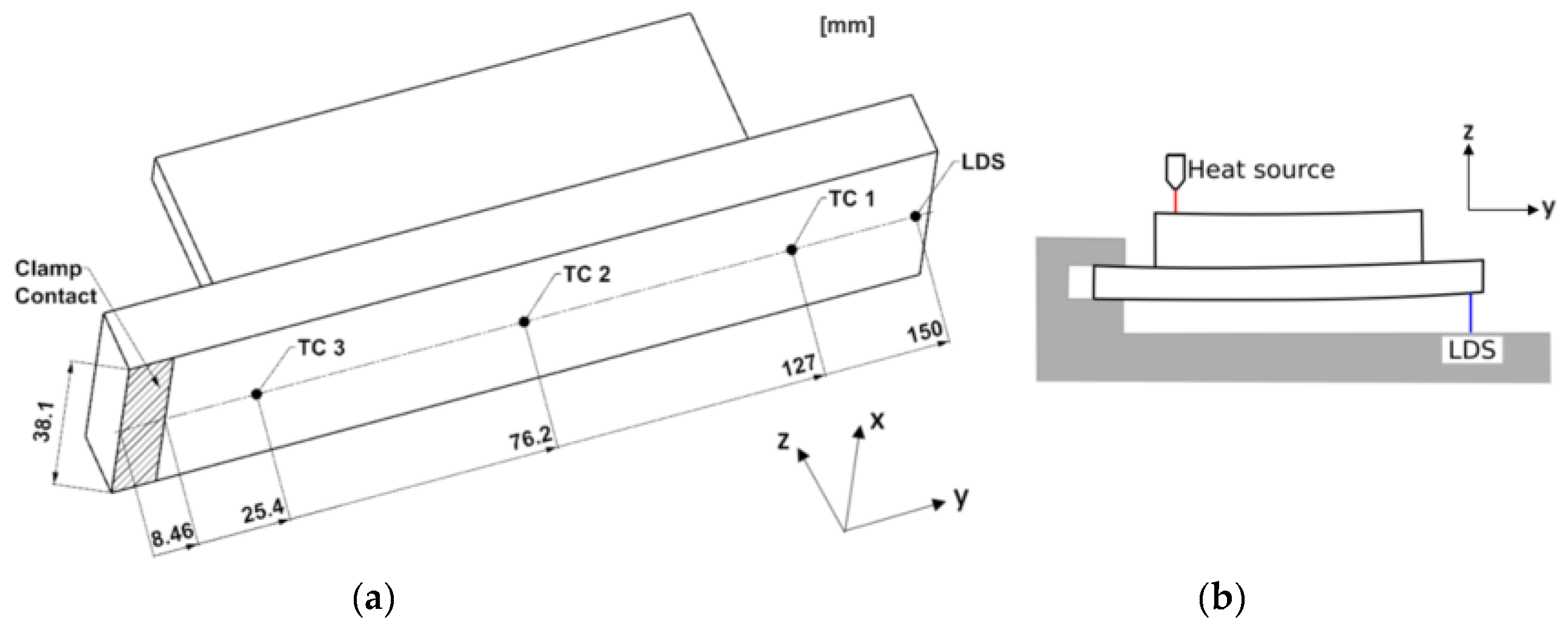
2.1. Experimental Set Up

The experiment used for validation was performed by Denlinger et al. [26]. In it, a wall was built on a substrate plate using directed energy deposition (DED). Two cases of DED of alloy 625 presented in that paper were selected for this work. They differed with respect to the dwell time between each layer. One case had no dwell time and the other had a dwell time of 20 s between each layer. The wall was 101.6 mm long, 38.1 mm high, and 6.7 mm wide, and the substrate plate was 152.4 mm long, 38.1 mm wide, and 12.7 mm thick. The deposit was made using a laser power of 2 kW and a scan speed of 10.6 mm/s. The wall consisted of 42 layers, and each layer was comprised of three passes. The layer thickness used in the simulations was 0.9 mm. Figure 1 shows the scan sequences during the deposition. Figure 1a shows the sequence for odd-numbered layers and Figure 1b shows the case for even-numbered layers.

The measurements of temperature, displacements, and residual stress were used to validate the simulations. The temperature was measured by three thermocouples and the deflections by a laser displacement sensor (LDS) at the positions shown in Figure 2a. The LDS measures the distortion of the substrate along the z-direction, see Figure 2b. The residual stress was measured at the location of TC2 using the hole drilling method defined in ASTM E837. The method has an accuracy of ±50 MPa if all requirements are met. The method measures the absolute residual stress at a point, including the residual stresses incurred when the material is prepared. The preparation of the substrate in the experiment is not specified in [26].

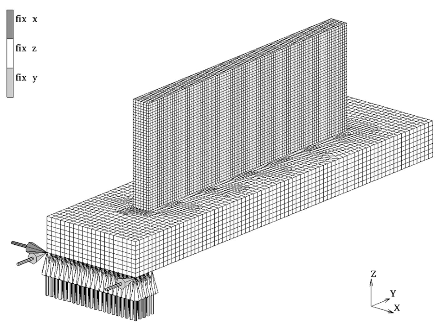
2.2. Computational Set Up

The finite element software MSC.Marc was used in the simulations. It accounts for large strains and deformations. A strong coupling between the thermal and mechanical analyses was obtained by the so-called staggered approach. For each time step the thermal problem was first solved and the resulting thermal load was used as an input to the mechanical problem. After the mechanical problem was solved, the geometry was updated. Thus, updating of the geometry in the thermal analysis lags one step behind. Moreover, the heat generation by the plastic deformation in the mechanical analysis was added to the thermal analysis in the next time step. For an AM simulation, that contribution was minimal. Eight-node hex elements, improved with the constant dilatation approach and assumed strain formulation, were used for the spatial discretization. The constant dilatation approach forces the volumetric strain to be constant throughout the element in order to avoid volume locking. With the assumed strain formulation, the interpolation functions were modified such that the shear strain variation could be better represented in the element. This improved the bending behavior compared to conventional hex element. Fixed time steps of 0.1 s and 0.2 s were used for the heat input and cooling phases respectively.

2.2.1. Material Models

The thermal and elastic properties versus temperature are listed in

Table 1. Temperature dependent properties of alloy 625.

Temp (°C)	Conductivity (W/mK) [39]	Expansion Coefficient (×10−6/°C)	Young’s Modulus (GPa) [29]	Temp (°C)	Specific Heat 1 (J/kg/°C) [30]
20	9.80	12.7	208	−18	402
100	11.2	13.2	-	21	410
200	12.8	13.8	199	93	427
300	14.4	14.6	192	204	456
400	16.3	15.4	186	316	481
500	17.3	16.7	179	427	511
600	19.3	18.0	171	538	536
700	21.0	19.2	163	649	565
800	22.6	20.4	153	760	590
900	24.6	21.6	142	871	620
1000	26.7	22.9	126	982	645
1189	-	25.3	-	1093	670
1250	-	-	10	1300	710
1300	32.0	-	-
1350	230	-	-

¹ The additional heat of fusion is indicated in the text.

. A cut-off was used for properties outside the given temperatures; i.e., the values were not extrapolated but instead the last given value was used. The thermal expansion coefficient in the table is the tangent coefficient based on data in [29,30]. The density was 8.44 g/cm³ [30]. The latent heat for melting and solidification was 150 kJ/kg in the temperature interval 1189–1336 °C [31]. This was obtained from an experiment where the latent heat was measured during solidification with a cooling rate of 60–100 °C/s. The solidus temperature was calculated as 1137 °C according to the Scheil module in Thermo-Calc [32]. The flow stress for the annealed state of the material was compiled from stress–strain curves from various sources [33,34,35], as indicated in

Table 2. Flow stress of alloy 625.

Temp (°C)	20	400	650	950	1000	1100	1200	1260
Reference	[33]	[34]	[33]	[35]	[35]	[35]	[35]	-
Plastic strain (−)	True stress (MPa)
0	490	402	370	116	75.0	37.0	15.0	1.0
0.005	510	460	373	178	100	50.4	23.2	1.2
0.01	529	490	380	222	115	63.8	31.4	1.4
0.015	548	514	388	250	137	76.3	39.3	1.6
0.02	568	532	401	270	151	88.7	46.1	1.8
0.03	610	568	432	290	171	102	52.6	2.0
0.05	684	627	489	320	207	113	58.4	2.2
0.08	777	697	576	340	223	119	62.4	2.4
0.12	891	789	665	350	226	122	60.2	2.6
0.2	1096	951	797	349	229	120	54.1	2.8
0.28	1272	1075	955	337	230	113	50.5	3.0

Bolded values: independent variables.

. The flow stress was tabulated versus plastic strain and temperature, which was used to interpolate flow stress and hardening of the material. The accumulated equivalent plastic strain was set to zero whenever the temperature was above 1137 °C. The removal of the accumulated plastic strain corresponds to the reduction in dislocation density, owing to both the melting and diffusion-controlled climb processes that annihilate dislocations, and thereby suppressed the hardening at high temperatures.

The material properties in this work were taken from experimental data. Physically based flow stress models and microstructure models were used to describe the physics in the material more accurately. These models were coupled to FE models for AM. Murgau et al. [36] and Salsi et al. [37] used microstructure models and were able to predict the amount of different phase fractions formed in the process. Babu et al. [38] coupled a microstructure model and a physically based flow stress model to the mechanical properties and applied it in a DED-process. They could thereby get a more accurate description of the material behavior over the temperature, strain rate, and strain range during the process.

2.2.2. Addition of Material

There are two basic approaches to model the addition of the filler material in AM simulations, quiet element and inactive element [14]. In the quiet element approach the elements of the filler material are included in the problem definition when the analysis starts but is given material properties that are scaled such that they do not affect the surrounding structure. When the filler material is added, the corresponding elements obtain the correct material properties. In the inactive element approach, the elements of the deposited material are not included in the problem definition before the material is added and the elements are activated. Michaleris et al. [40] proposed a hybrid quiet/inactive element approach. Initially all elements were set to inactive. Then, layer by layer, all elements in the current layer were switched to quiet. The individual elements obtained the correct material properties when the corresponding material was added in the process. In that approach, the system of equations is recomputed only when each layer is activated.

The inactive element approach was used in the current work. The activation of elements is performed in two steps. They are first activated in the thermal analysis in order to supply heat to the elements. The position of the heat source determines which elements will be activated in the thermal step. A search algorithm is used to locate these elements. The subsequent mechanical activation is temperature controlled. When the temperature decreases below the solidification temperature (T_solidus) for the material, the element is activated in the mechanical analysis.

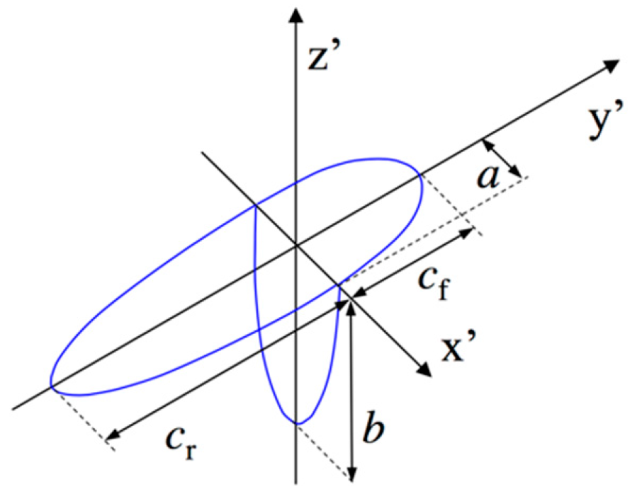
2.2.3. Heat Source Model

The heat source model prescribes the heat input. It should represent the resulting heat input from the heat source, which in this case is a laser. Different models with different geometries and heat distributions exist. Simpler models use constant heat applied in a certain geometry [41]. The intensity of the beam at the surface in the simulated experiment was determined to have a Gaussian profile [26]; thus, a model with Gaussian heat distribution was appropriate. Pavelic et al. [42] proposed a model with a planar Gaussian heat distribution at the surface. For more deep penetration processes a conical heat source, or a combination of two heat sources proposed by Lundbäck et al. [43] can be preferred. However, in this work the heat flux of the laser, which was in convective mode, was modeled by the double ellipsoidal heat source model proposed by Goldak et al. [44]. This model has been used extensively for modeling the heat input of both arc and beam heat sources. In the simulation of the current case by Denlinger et al. [3] they also used this heat input model.

The double ellipsoidal heat source model is described by a moving local coordinate system. The heat source is moving in the $y^{\prime }$-direction according to Figure 3. The heat source consists of two elliptic regions, one at the front of the origin, described by Equation (1),

$$q_f\left(x,y,z\right)=\frac{6\sqrt{3}{f}_{f}Q}{ab{c}_f{\pi }^{3/2}}{e}^{-3{\left(\frac{x^{\prime }}{a}\right)}^2}{e}^{-3{\left(\frac{y^{\prime }}{c_f}\right)}^2}{e}^{-3{\left(\frac{z^{\prime }}{b}\right)}^2}$$

(1)

and one behind the origin, described by Equation (2),

$$q_r\left(x,y,z\right)=\frac{6\sqrt{3}{f}_{r}Q}{ab{c}_r{\pi }^{3/2}}{e}^{-3{\left(\frac{x^{\prime }}{a}\right)}^2}{e}^{-3{\left(\frac{y^{\prime }}{c_r}\right)}^2}{e}^{-3{\left(\frac{z^{\prime }}{b}\right)}^2}.$$

(2)

$a$, $b$, $c_f$, and $c_r$ are shown in Figure 3. These parameters and the net heat input, Q, were determined by calibration and the values are listed in

Table 3. Calibrated and given parameters.

hfixture (W m−2 K−1)	h (W m−2 K−1)	E	η	a (m)	b (m)	cf (m)	cr (m)
500	11	0.45	0.29	0.002	0.002	0.002	0.004

. The parameters $f_f$ and $f_r$ must comply with

$$f_f+f_r=2.$$

(3)

The heat flux should be continuous along $y^{\prime }$ = 0 in Figure 3, which together with Equation (3) gives Equations (4) and (5),

$$f_f=\frac{2c_f}{c_f+c_r}$$

(4)

$$f_r=\frac{2c_r}{c_f+c_r}.$$

(5)

The integration of the heat input Equations (1) and (2) gives the total heat input in a time step that may vary as it is evaluated over the integration points in the elements of the mesh. Thus, the heat input may fluctuate depending on where the heat source is located with respect to the mesh. These fluctuations are avoided by controlling the heat input in every iteration in every time step, according to Lindgren [14].

2.2.4. Simulation Models

All of the 126 weld passes were simulated individually in two more accurate models. The two models differed with respect to the size of the elements. The results from the model with a finer mesh acted as a reference, and they were compared with those from the experiments. Subsequently, the results of the lumped models were compared with those reference results. The reference model is shown in Figure 4, and it consists of 43,312 elements with 184 elements per weld pass. The motivation for the model with the coarser mesh was to evaluate the efficiency gained owing to the lumping only, excluding the reduction in number of elements. This model is shown in Figure 5b, and it consists of 7683 elements with 46 elements per weld pass.

The mechanical boundary conditions used for all the models are shown in Figure 4. The nodes at the bottom of the substrate in contact with the clamp are fixed in the z-direction. Two nodes at the corner are fixed in the y-direction and one node in the x-direction, as seen in Figure 4, to prevent rigid body motion. The thermal boundary conditions are convection and radiation, which were applied on all free faces except at the top faces of the added material. The heat transfer at the interface between the substrate and the fixture is explained in the next section.

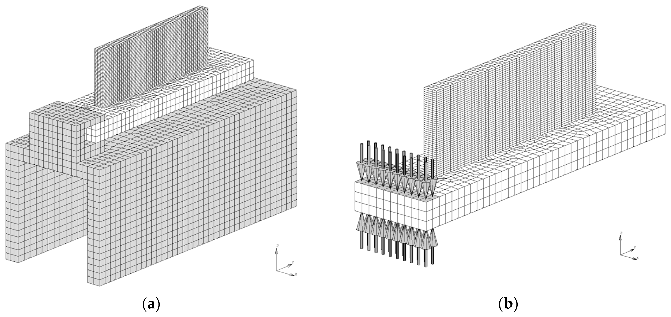
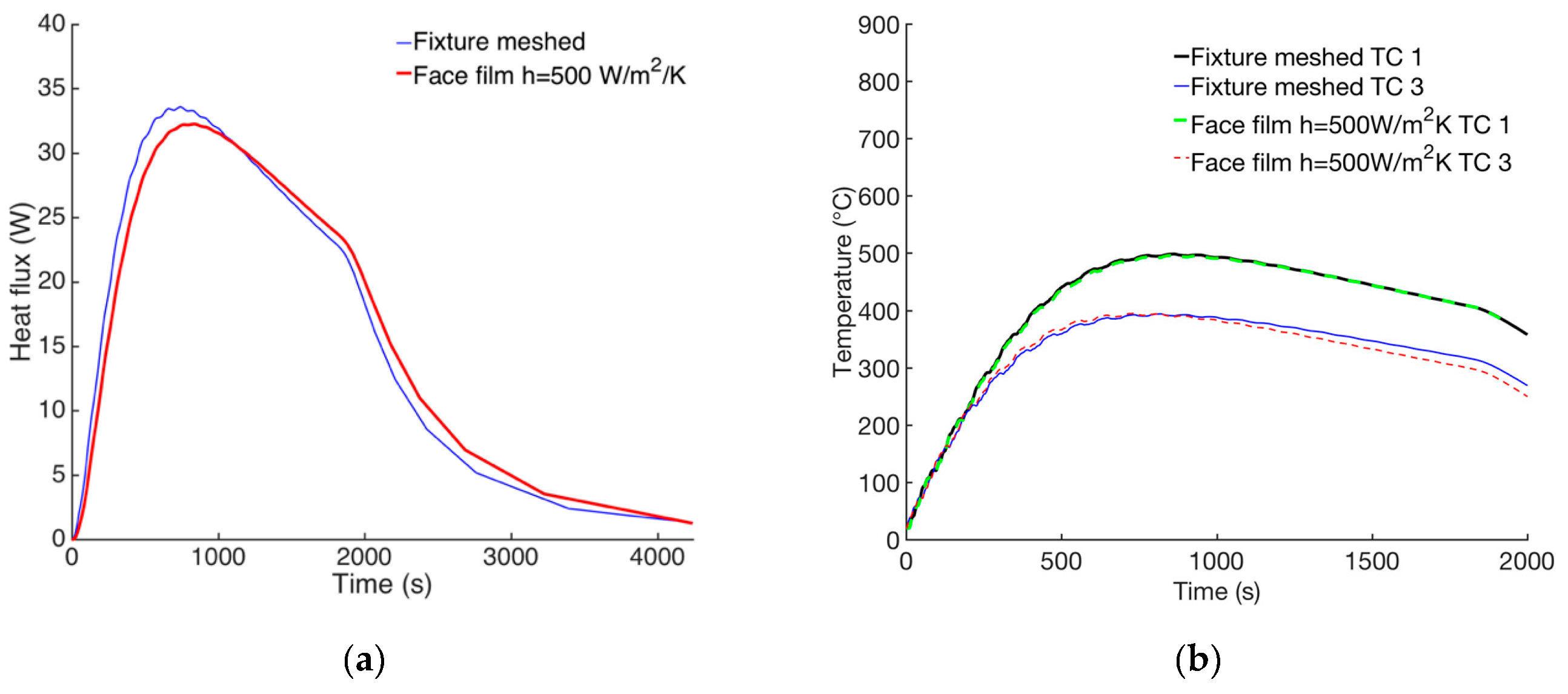
2.2.5. Heat Transfer Through Fixture

The heat transfer at the interface between the substrate and the fixture (see Figure 5a) was modeled by a large value of the heat transfer coefficient. The model shown in Figure 5a includes the fixture, whereas the fixture is replaced by a boundary condition in the model in Figure 5b, in order to reduce the size of the model. The heat loss to the fixture was modeled as a convective heat transfer with a convection coefficient, h_fixture, of 500 W/m². This value was obtained by the calibration procedure described below.

The total heat loss through the interfaces between the base plate and the fixture, and the temperatures in thermocouples TC 1 and TC 3, were compared for the two models. The value of the convective heat transfer coefficient was adjusted until the heat flux through the fixture interface and the temperatures in TC1 and TC3 were in good agreement; see Figure 6.

2.2.6. Calibrated Parameters

The computed temperatures from the reference model with the fine mesh were compared with those from the experiments to calibrate the parameters included in Table 3. These values were used for all the models. The heat transfer between the substrate and the fixture, denoted as h_fixture, has been discussed earlier. The heat loss to the ambient air is described by the film coefficient h and the emissivity is denoted by e. These values were calibrated with respect to the final cooling part of the temperature measurements and were in agreement with the general guidelines in the heat transfer literature. The heat source efficiency η indicates how much of the total power of the laser is absorbed by the material. The heat distribution is described by the estimated heat source dimension parameters, a, b, and c, according to Figure 3. These parameters, together with the efficiency parameter, are determinants for the obtained peak temperatures.

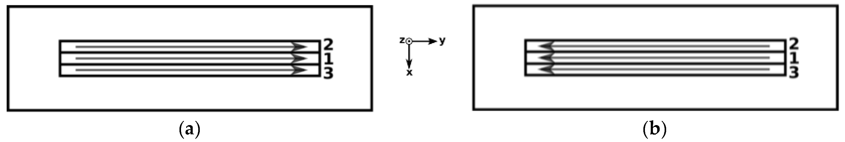
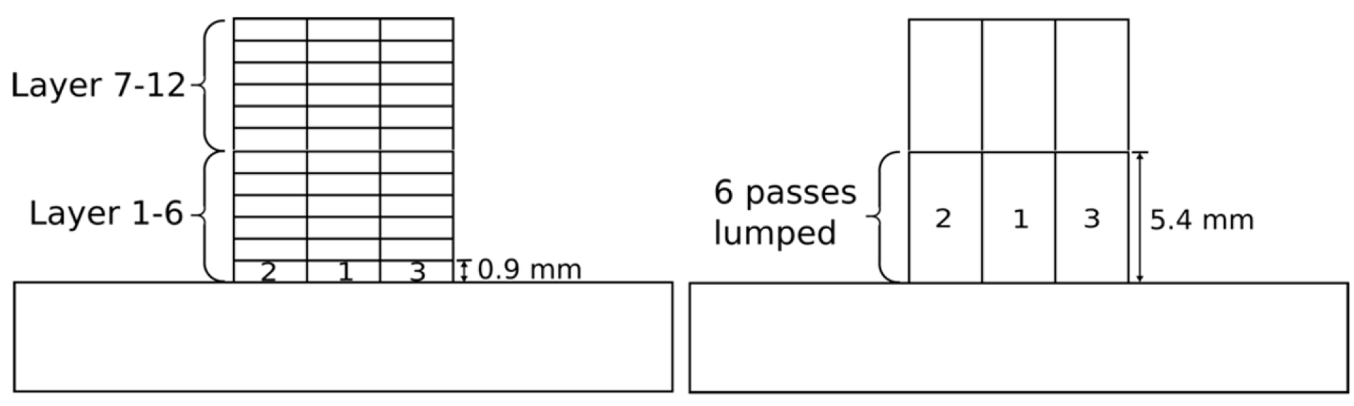
2.2.7. Lumping of Passes in AM Simulations

The coarse model shown in Figure 5b still requires considerable computing time. The effect of the lumping of welds has been studied with respect to efficiency and accuracy. The lumping procedure is explained with reference to the specific case of lumping six weld passes into one. The lumped model was created by merging six passes in the height direction into one. A general sketch of the lumping procedure can be seen in Figure 7. The largest element size in the height direction was determined by the layer thickness. In this case, there was the possibility to coarsen the mesh when lumping was utilized.

The only parameters that needed to be changed were the heat source velocity v, time step length Δt, and cooling time t_c. All other parameters, such as heat source geometry and effect, were kept unchanged. The changes of the three parameters were both physically sound and straight forward. The velocity was divided by the number of lumped passes, n, and the time step length was multiplied by n. The heat source then moved the same distance during each time step, regardless of how many passes are lumped. The modified parameters are summarized in

Table 4. Changed time and velocity settings when lumping passes.

	Detailed Model	Lumping n Passes
Time step	Δt	Δt* = Δt·n
Heat source speed	v	v* = v/n
Total Time for welding case	tw	tw* = tw·n
Total Time for cooling case	tc	tc* = tc·n

for an arbitrary number of lumped passes. This means that the energy per unit length of a weld was the sum of those for the individual passes. The total energy supplied to the model was the same for all cases.

The principle of lumping is shown in Figure 8. As can be seen, the number of the elements representing the added layer can be reduced when lumping is applied. The number of elements for the various case models is listed in

Table 5. Number of elements for the simulation models.

	Number of Elements	Number of Nodes
Model with fine mesh	43,312	50,859
Model with coarse mesh	7683	10,608
Lumping 3 passes	3819	5344
Lumping 6 passes	3819	5344
Lumping 14 passes	3543	4968

.

3. Results

The results for the detailed model with fine mesh and the reduced models with lumped passes are described here. The model with the fine mesh was validated with measurements and acts as a reference model for the lumped models. Further, the reduction of simulation time with the lumped models is described.

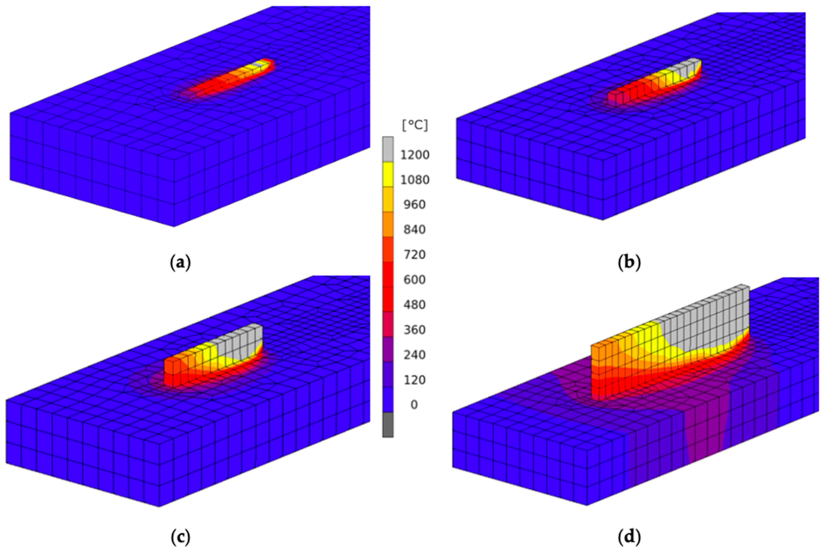
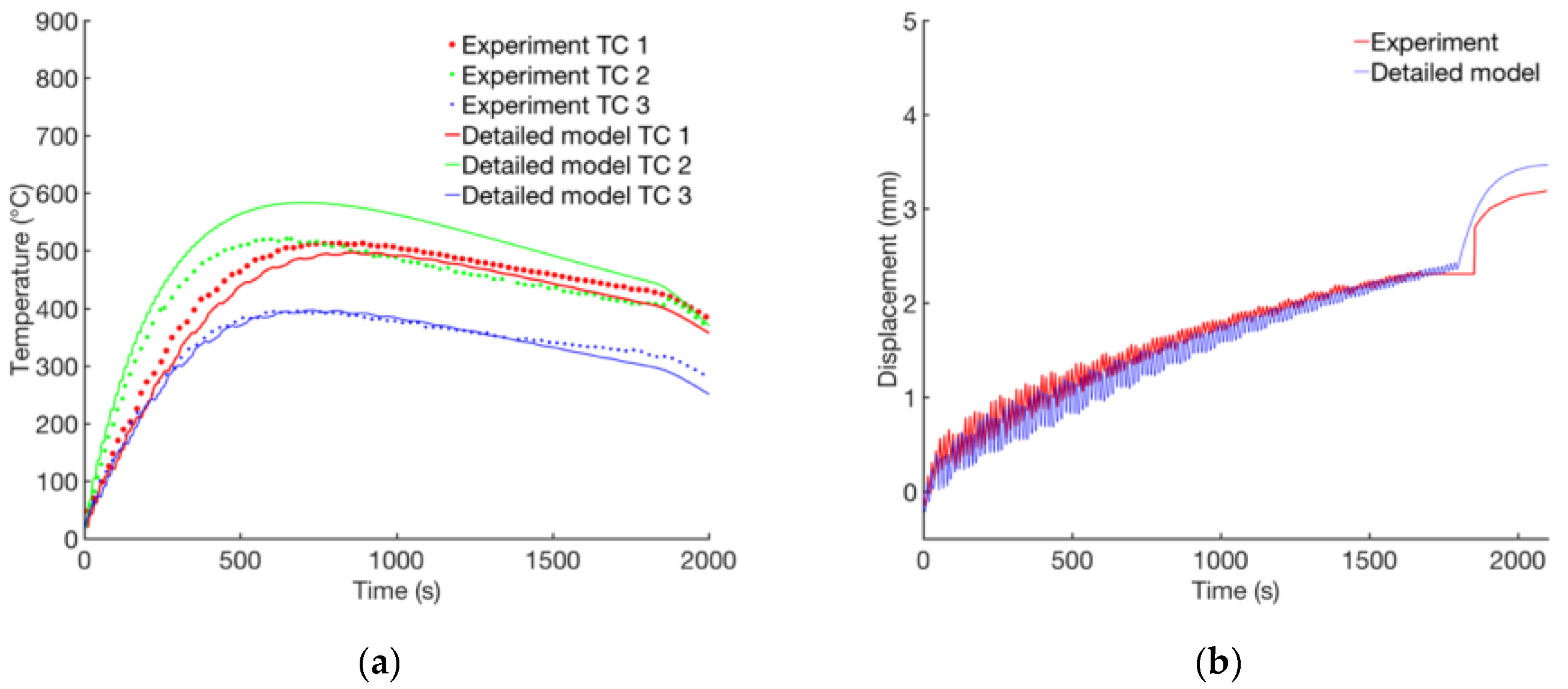
3.1. Results for Reference Model

The results for the calibrated simulation model with the fine mesh (see Figure 4) are shown here. The simulation was compared with the temperature and displacement measurements from [26] for the cases with no dwell time and with 20 s dwell time between layers. Figure 9 shows the temperature and displacement results for the case with no dwell time, whereas Figure 10 shows the temperature and displacement results for the case with 20 s dwell time between layers.

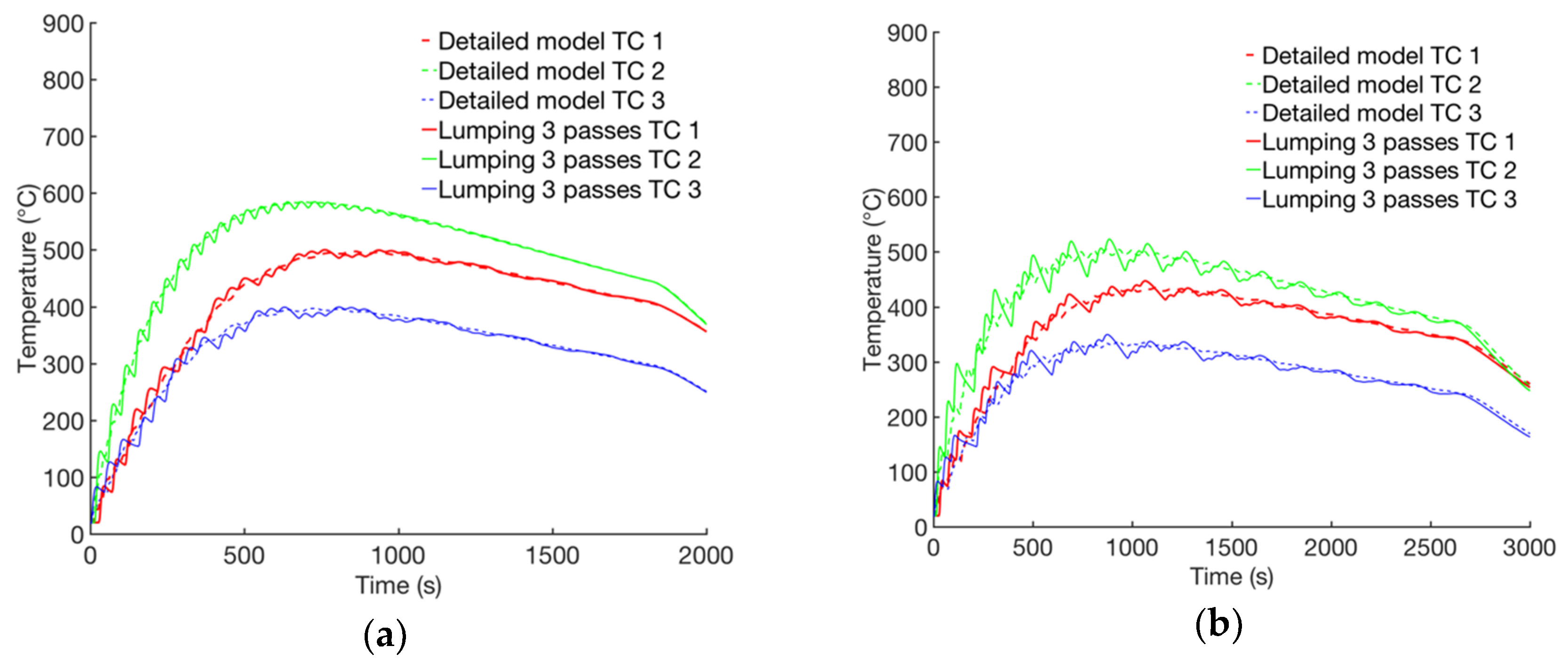
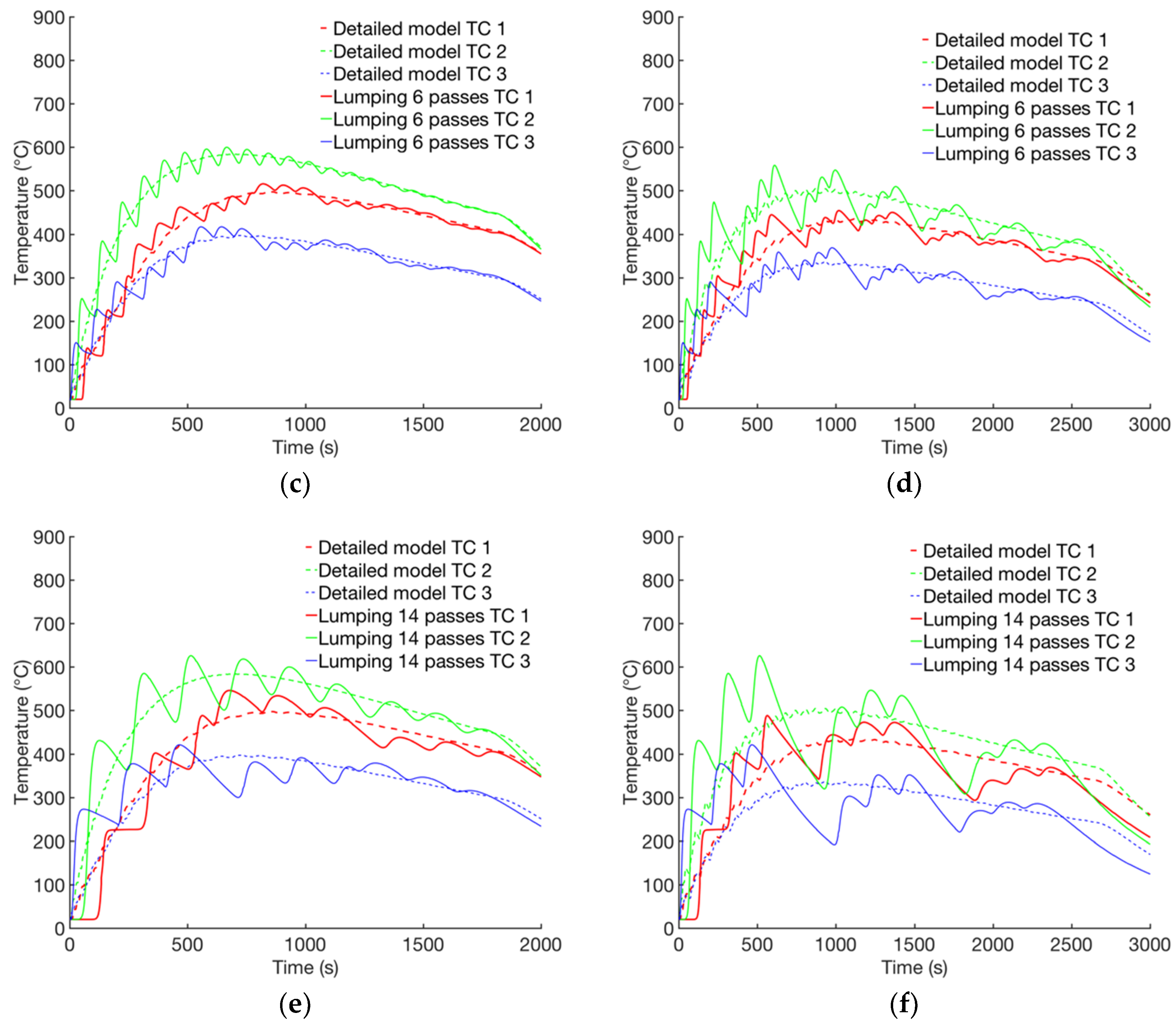
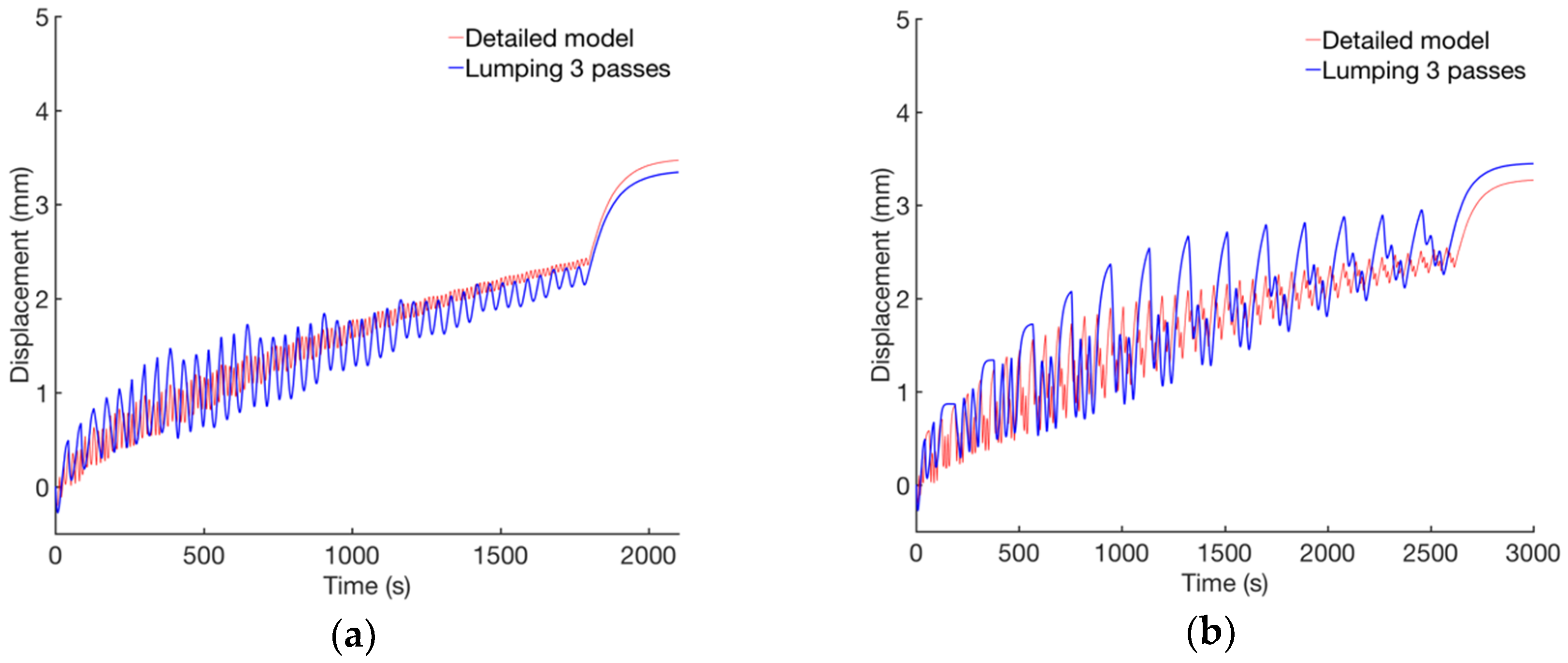
3.2. Result for Lumped Models

The main aim of this study was to evaluate the modeling error that is introduced when using the described method of lumping weld passes, and the reduction in computation time. The transient temperature and displacement during the process and the residual stress were evaluated for the lumped models. When the results were compared, the same locations as in the measurements were used for the lumped models and for the reference model with fine mesh.

The temperatures are compared at the locations of the thermocouples in the experiment; see Figure 2a. The temperature results for the cases with no dwell time and with 20 s dwell time between layers for lumping of 3, 6, and 14 passes are shown in Figure 11. They are compared with the reference model with fine mesh, which is denoted in the figure as the detailed model.

The displacement at the location of the LDS measurement in the experiment is shown below. The results for the cases with no dwell time and with 20 s dwell time between layers for lumping of 3, 6, and 14 passes are shown in Figure 12 and are compared with the reference model with fine mesh, denoted in the figure as the detailed model. The final displacement for the reference model with fine mesh and the lumped models are collected in

Table 6. Final displacement and relative deviation for all models.

	No Dwell Time Between Layers		20s Dwell Time Between Layers
	Final Displacement (mm)	Relative Deviation (%)	Final Displacement (mm)	Relative Deviation (%)
Model with fine mesh	3.61	Reference = 0	3.43	Reference = 0
Lumping 3 passes	3.50	3.0	3.59	4.7
Lumping 6 passes	3.69	2.2	3.95	15.2
Lumping 14 passes	3.74	3.6	3.88	13.1

. The table also shows the relative deviation.

The computed residual stresses at the mid cross section in the weld direction are compared. Only the results for the case with no dwell time and 3, 6, and 14 passes are shown in Figure 13. They are nearly identical to the results for the cases with 20 s dwell time. Moreover, the residual stress in the welding direction at the bottom center of the substrate was compared with that in the experimental results and is presented in

Table 7. Residual stress in the welding direction at the bottom center of the substrate in the case with no dwell time between layers.

	Residual Stress in the Welding Direction (MPa)
Experiment	740
Model with fine mesh	508
Lumping 3 passes	453
Lumping 6 passes	447
Lumping 14 passes	449

.

3.3. Computation Times

The computation times for the different simulations are compiled in

Table 8. Computation time for the simulation models.

		Computation Time	Computation Time (%)
No dwell time between layers	Model with fine mesh	4 d 16 h 39 min	956
	Model with coarse mesh	11 h 47 min	Reference = 100
	Lumping three passes	2 h 24 min	20.4
	Lumping six passes	1 h 3 min	8.9
	Lumping 14 passes	29 min	4.1
20s dwell time between layers	Model with fine mesh	5 d 11 h 38 min	961
	Model with coarse mesh	13 h 42 min	Reference = 100
	Lumping three passes	2 h 25 min	17.6
	Lumping six passes	1 h 10 min	8.5
	Lumping 14 passes	29 min	3.5

. The table also contains the computation times in percentages for the lumping models, with the model with coarse mesh as the reference. For all simulations, multithreading with four threads has been used when solving the resulting system of equations on a machine with the Intel Xenon E5-2670, 2.6 GHz chip.

4. Discussion

The simulated results from the detailed model with respect to temperature and displacement are in good agreement with the measurements. However, the temperature at the TC 2 location in the case with no dwell time between layers is an exception. This can be seen in Figure 9a; the temperature registered by TC 2 is higher than that registered by TC 1 at the beginning, but it then decreases so that the two curves cross after around 1000 s according to the measurements in [26]. This behavior is not shown in the simulation and there is no realistic explanation for this occurrence. None of the other similar cases in [26] show this behavior.

The residual stress at the mid cross section of the substrate for the simulation was 508 MPa, a value that can be compared with the measured value of 740 MPa. Denlinger et al. [3] performed a similar simulation and obtained a residual stress of just above 500 MPa. They explain the difference between the simulation and measurements with the temperature-dependent precipitation hardening that the simulation model does not take into account.

The main focus of this study was to evaluate the trade-off between accuracy and computation time. It is clear that lumping welds can be used to reduce the computation time significantly for the studied case, as presented in Table 8. This is also relevant for other geometries with large number of passes.

The extent of lumping depends on the aim of the model and the required accuracy. The temperature results for lumping show that lumping a larger number of passes generates larger oscillations. However, the overall trend is captured even in the case of lumping 14 passes. The displacement results show similar behavior to that of the temperatures. The results show that the final deformation of a built product can be predicted accurately, even when lumping 14 passes. The overall residual stress distribution is captured but the magnitude at the evaluated location is already 10% lower when lumping three passes.

The procedure described for lumping weld passes of the DED process is straightforward. Once the accurate thermo-mechanical model is created, no additional calibrations are needed to set up a model using the lumping technique. The only parameters that need to be changed are the heat source velocity, v, time step length, Δt, and cooling time, t_c. These parameters are changed in a predefined way. The element size is also made larger for the lumped models to further reduce the computation time. However, the element size must always be estimated in a FE-model.

The results also show that the lumping technique works better for the cases without dwell time, which correspond to the left column in Figure 12. The final displacements deviate more when there is a dwell time between each pass; see Table 6. The reason is that the procedure applied will extend the dwell time with a multiple corresponding to the number of lumped passes. Because of this, the material is cooled down excessively before the next layer is added. This mismatch in temperature between the existing material and the added filler material causes additional plasticity. A better prediction of the final geometry is achieved if the time schedule of the added welds is adjusted so that cooling of the existing material is more similar to that in the real process. The drawback with that approach is that a lumped model is needed to estimate this beforehand. An example of this is shown in Figure 14, where the original approach is compared with a simulation in which the dwell time is halved.

Depending on the scope of the simulation, the large oscillations in the temperature and displacement results owing to lumping may be acceptable or not. If the scope is to predict the final deformation and residual stress state, it has been shown that lumping can be applied with sustained accuracy. However, if the microstructure is of interest, then lumping would not be a viable way to reduce the computational time, as it alters the thermal history in a deleterious way.

5. Conclusions

A thermo-mechanical FE model has been validated with temperature and displacement results from a DED process for alloy 625. The validated model has then been used to study lumping of welds with respect to efficiency and accuracy. Based on the given AM process and material, the following specific conclusions can be drawn from this work:

• Lumping of welds can reduce the computational time considerably, owing to the reduction in number of time steps and the reduction of number of elements required in the model.
• Lumping of welds is a viable option when the main scope is to capture the overall residual states, such as stresses and deformations, of an AM-produced component.
• The heat source parameters do not have to be re-calibrated for the different lumping cases. The velocity is the only parameter that changed. The velocity is divided by the number of lumped layers to get a correct input of energy per length unit.
• History-dependent results, such as microstructure evolution, cannot be predicted when applying the lumping technique, since the local thermal history is not captured.

References

1. Herderick, E. Additive manufacturing of metals: A review. In Proceedings of the Materials Science and Technology 2011, Columbus, OH, USA, 16–20 October 2011; Volume 2, pp. 1413–1425. [Google Scholar]
2. Lundbäck, A.; Lindgren, L.-E. Modelling of metal deposition. Finite Elem. Anal. Des. 2011, 47, 1169–1177. [Google Scholar] [CrossRef]
3. Denlinger, E.R.; Michaleris, P. Effect of stress relaxation on distortion in additive manufacturing process modeling. Addit. Manuf. 2016, 12, 51–59. [Google Scholar] [CrossRef] [Green Version]
4. Montevecchi, F.; Venturini, G.; Scippa, A.; Campatelli, G. Finite element modelling of wire-arc-additive-manufacturing process. Procedia CIRP 2016, 55, 109–114. [Google Scholar] [CrossRef] [Green Version]
5. Zhao, H.; Zhang, G.; Yin, Z.; Wu, L. Three-dimensional finite element analysis of thermal stress in single-pass multi-layer weld-based rapid prototyping. J. Mater. Process. Technol. 2012, 212, 276–285. [Google Scholar] [CrossRef]
6. Chiumenti, M.; Cervera, M.; Salmi, A.; Agelet de Saracibar, C.; Dialami, N.; Matsui, K. Finite element modeling of multi-pass welding and shaped metal deposition processes. Comput. Methods Appl. Mech. Eng. 2010, 199, 2343–2359. [Google Scholar] [CrossRef]
7. Umer, U.; Ameen, W.; Abidi, M.H.; Moiduddin, K.; Alkhalefah, H.; Alkahtani, M.; Al-Ahmari, A. Modeling the effect of different support structures in electron beam melting of titanium alloy using finite element models. Metals 2019, 9, 806. [Google Scholar] [CrossRef] [Green Version]
8. Denlinger, E.R.; Irwin, J.; Michaleris, P. Thermomechanical modeling of additive manufacturing large parts. J. Manuf. Sci. Eng. 2014, 136, 061007. [Google Scholar] [CrossRef]
9. Denlinger, E.R.; Gouge, M.; Irwin, J.; Michaleris, P. Thermomechanical model development and in situ experimental validation of the Laser Powder-Bed Fusion process. Addit. Manuf. 2017, 16, 73–80. [Google Scholar] [CrossRef]
10. Lindwall, J.; Malmelöv, A.; Lundbäck, A.; Lindgren, L.-E. Efficiency and accuracy in thermal simulation of powder bed fusion of bulk metallic glass. JOM 2018, 70, 1598–1603. [Google Scholar] [CrossRef]
11. Patil, N.; Pal, D.; Khalid Rafi, H.; Zeng, K.; Moreland, A.; Hicks, A.; Beeler, D.; Stucker, B. A generalized feed forward dynamic adaptive mesh refinement and derefinement finite element framework for metal laser sintering—Part I: Formulation and algorithm development. J. Manuf. Sci. Eng. 2015, 137, 041001. [Google Scholar] [CrossRef]
12. Pal, D.; Patil, N.; Kutty, K.H.; Zeng, K.; Moreland, A.; Hicks, A.; Beeler, D.; Stucker, B. A generalized feed-forward dynamic adaptive mesh refinement and derefinement finite-element framework for metal laser sintering—Part II: Nonlinear thermal simulations and validations 2. J. Manuf. Sci. Eng. 2016, 138, 061003. [Google Scholar] [CrossRef]
13. Lindgren, L.-E. Finite element modeling and simulation of welding. Part 3: Efficiency and integration. J. Therm. Stress. 2001, 24, 305–334. [Google Scholar] [CrossRef]
14. Lindgren, L.-E. Computational Welding Mechanics. Thermomechanical and Microstructural Simulations; Woodhead Publishing in Materials: Cambridge, UK, 2007. [Google Scholar]
15. Chiumenti, M.; Lin, X.; Cervera, M.; Lei, W.; Zheng, Y.; Huang, W. Numerical simulation and experimental calibration of additive manufacturing by blown powder technology. Part I: Thermal analysis. Rapid Prototyp. J. 2017, 23, 448–463. [Google Scholar] [CrossRef] [Green Version]
16. Prabhakar, P.; Sames, W.J.; Dehoff, R.; Babu, S.S. Computational modeling of residual stress formation during the electron beam melting process for Inconel 718. Addit. Manuf. 2015, 7, 83–91. [Google Scholar] [CrossRef] [Green Version]
17. Keller, N.; Neugebauer, F.; Xu, H.; Ploshikhin, V. Thermo-mechanical simulation of additive layer manufacturing of titanium aerospace structures. In Proceedings of the LightMAT Conference, Bremen, Germany, 3 September 2013. [Google Scholar]
18. Neugebauer, F.; Keller, N.; Ploshikhin, V.; Feuerhahn, F.; Köhler, H. Multi scale fem simulation for distortion calculation in additive manufacturing of hardening stainless steel. In Proceedings of the International Workshop on Thermal Forming and Welding Distortion, Bremen, Germany, 9–10 April 2014. [Google Scholar]
19. Keller, N.; Ploshikhin, V. New method for fast prediction of residual stress and distortion of AM parts. In Proceedings of the Solid Freeform Fabrication Symposium, Austin, TX, USA, 4–6 August 2014; pp. 1229–1237. [Google Scholar]
20. Liang, X.; Chen, Q.; Cheng, L.; Yang, Q.; To, A. A modified inherent strain method for fast prediction of residual deformation in additive manufacturing of metal parts. In Proceedings of the 28th Annual International Solid Freeform Fabrication Symposium, Austin, TX, USA, 7–9 August 2017; pp. 2539–2545. [Google Scholar]
21. Ueda, Y.; Yuan, M. Prediction of residual stresses in butt-welded plates using inherent strain. ASME J. Eng. Mater. Technol. 1993, 115, 417–423. [Google Scholar] [CrossRef]
22. Ueda, Y. Predicting and measuring methods of two- and three-dimensional welding residual stresses by using inherent strain as a parameter. In Modeling in Welding, Hot Powder Forming and Casting; ASM International: Cleveland, OH, USA, 1997; pp. 91–113. [Google Scholar]
23. Murakawa, H.; Luo, Y.; Ueda, Y. Inherent strain as an interface between computational welding mechanics and its industrial application. In Mathematical Modelling of Weld Phenomena 4; Institute of Materials: Graz, Austria, 1998; pp. 597–619. [Google Scholar]
24. Li, C.; Fu, C.; Guo, Y.; Fang, F. A multiscale modeling approach for fast prediction of part distortion in selective laser melting. J. Mater. Process. Technol. 2016, 229, 703–712. [Google Scholar] [CrossRef]
25. Li, C.; Fu, C.H.; Guo, Y.B.; Fang, F.Z. Fast prediction and validation of part distortion in selective laser melting. Procedia Manuf. 2015, 1, 355–365. [Google Scholar] [CrossRef] [Green Version]
26. Denlinger, E.R.; Heigel, J.C.; Michaleris, P.; Palmer, T.A. Effect of inter-layer dwell time on distortion and residual stress in additive manufacturing of titanium and nickel alloys. J. Mater. Process. Technol. 2015, 215, 123–131. [Google Scholar] [CrossRef]
27. De Oliveira, M.M.; Couto, A.A.; Almeida, G.F.C.; Reis, D.A.P.; De Lima, N.B.; Baldan, R. Mechanical behavior of inconel 625 at elevated temperatures. Metals 2019, 9, 301. [Google Scholar] [CrossRef] [Green Version]
28. Anam, M.A.; Pal, D.; Stucker, B. Modeling and experimental validation of nickel-based super alloy (Inconel 625) made using selective laser melting. In Proceedings of the 24th International Solid Freeform Fabrication Symposium—An Additive Manufacturing Conference, Austin, TX, USA, 12–14 August 2013; pp. 463–473. [Google Scholar]
29. Haynes 625 Alloy Brochure. Available online: http://haynesintl.com/docs/default-source/pdfs/new-alloy-brochures/high-temperature-alloys/brochures/625-brochure.pdf?sfvrsn=12 (accessed on 5 November 2019).
30. INCONEL alloy 625—Special Metals. Available online: https://www.specialmetals.com/assets/smc/documents/alloys/inconel/inconel-alloy-625.pdf (accessed on 5 November 2019).
31. Tinoco, J.; Fredriksson, H. Solidification of a modified inconel 625 alloy under different cooling rates. High Temp. Mater. Process. 2004, 23, 13–24. [Google Scholar] [CrossRef]
32. Hu, Y.L.; Lin, X.; Yu, X.B.; Xu, J.J.; Lei, M.; Huang, W.D. Effect of Ti addition on cracking and microhardness of Inconel 625 during the laser solid forming processing. J. Alloys Compd. 2017, 711, 267–277. [Google Scholar] [CrossRef]
33. Suave, L.M.; Bertheau, D.; Cormier, J.; Villechaise, P.; Soula, A.; Hervier, Z.; Hamon, F.; Laigo, J. Impact of thermomechanical aging on alloy 625 high temperature mechanical properties. In Proceedings of the Proceedings of the 8th International Symposium on Superalloy 718 and Derivatives, Pittsburgh, PA, USA, 28 September–1 October 2014. [Google Scholar]
34. Levin, B.F.; Dupont, J.N.; Marder, A.R. Robotic Weld Overlay Coatings for Erosion Control; Lehigh University, Energy Research Center: Washington, DC, USA, 1994. [Google Scholar]
35. Guo, S.; Li, D.; Guo, Q.; Wu, Z.; Peng, H.; Hu, J. Investigation on hot workability characteristics of Inconel 625 superalloy using processing maps. J. Mater. Sci. 2012, 47, 5867–5878. [Google Scholar] [CrossRef]
36. Murgau, C.C.; Lundbäck, A.; Akerfeldt, P.; Pederson, R. Temperature and microstructure evolution in gas tungsten arc welding wire feed additive manufacturing of Ti-6Al-4V. Materials 2019, 12, 3534. [Google Scholar] [CrossRef] [PubMed] [Green Version]
37. Salsi, E.; Chiumenti, M.; Cervera, M. Modeling of microstructure evolution of Ti6Al4V for additive manufacturing. Metals 2018, 8, 633. [Google Scholar] [CrossRef] [Green Version]
38. Babu, B.; Lundbäck, A.; Lindgren, L.-E. Simulation of Ti-6Al-4V additive manufacturing using coupled physically based flow stress and metallurgical model. Materials 2019, 12, 3844. [Google Scholar] [CrossRef] [PubMed] [Green Version]
39. Isolthermics Nicrofer 6020 hMo—Alloy 625. Available online: http://www.isolthermics.com.au/metals/pdfs/common-tech/Alloy 625 6020hMo.pdf (accessed on 5 November 2019).
40. Michaleris, P. Modeling metal deposition in heat transfer analyses of additive manufacturing processes. Finite Elem. Anal. Des. 2014, 86, 51–60. [Google Scholar] [CrossRef]
41. Contuzzi, N.; Campanelli, S.L.; Ludovico, A.D. 3D finite element analysis in the selective laser melting process. Int. J. Simul. Model. 2011, 10, 113–121. [Google Scholar] [CrossRef]
42. Pavelic, V.; Tanbakuchi, R.; Uyehara, O.A.; Myers, P.S. Experimental and computed temperature histories in gas tungsten arc welding of thin plates. Weld. J. Res. Suppl. 1969, 48, 295–305. [Google Scholar]
43. Lundbäck, A.; Runnemalm, H. Validation of three-dimensional finite element model for electron beam welding of Inconel 718. Sci. Technol. Weld. Join. 2005, 10, 717–724. [Google Scholar] [CrossRef]
44. Goldak, J.; Chakravarti, A.; Bibby, M. A new finite element model for welding heat sources. Metall. Trans. B 1984, 15, 299–305. [Google Scholar] [CrossRef]
45. Lindgren, L.E.; Lundbäck, A.; Fisk, M.; Pederson, R.; Andersson, J. Simulation of additive manufacturing using coupled constitutive and microstructure models. Addit. Manuf. 2016, 12, 144–158. [Google Scholar] [CrossRef]
Figure 1. Laser scan sequences during the deposition for (a) odd-numbered layers and (b) even-numbered layers. The arrows show the scanning direction, and the numbers, 1–3, show in which order the passes are done.
Metals 10 00058 g001
Figure 2. (a) Substrate and wall showing the location of the thermocouples (TC) and the laser displacement sensor (LDS) measurement at the bottom side of the substrate. (b) Sketch showing the position of the LDS distortion measurement.
Metals 10 00058 g002
Figure 3. Double ellipsoidal heat source [45].
Metals 10 00058 g003
Figure 4. Model with fine mesh. The arrows indicate the mechanical boundary conditions used for all models.
Metals 10 00058 g004
Figure 5. Simulation models. In (a) the fixture is meshed and in (b) the fixture is replaced by a convective boundary condition represented by the arrows.
Metals 10 00058 g005
Figure 6. Comparison of the total heat loss from baseplate to fixture (a) and the temperature in positions TC 1 and TC 3 (b) for the model with meshed fixture and the model with the fixture replaced by a convective boundary condition.
Metals 10 00058 g006
Figure 7. Sketch showing how the passes can be lumped.
Metals 10 00058 g007
Figure 8. The first pass added in the simulation. The legend is expressed in °C. (a) No lumping for the model with coarse mesh. The height corresponds to the real thickness of one DED layer. (b) Lumping of three layers. The height corresponds to the thickness of three DED layers. (c) Lumping of six layers. (d) Lumping of 14 layers.
Metals 10 00058 g008
Figure 9. Temperatures (a) and displacements (b) from measurements and model with fine mesh and no dwell time between layers.
Metals 10 00058 g009
Figure 10. Temperatures (a) and displacements (b) from measurements and model with fine mesh and 20 s dwell time between layers.
Metals 10 00058 g010
Figure 11. The computed temperatures for the model with fine mesh are compared with those for models with lumping of 3, 6, and 14 passes. The models with no dwell time between layers are shown in (a), (c) and (e) whereas (b), (d) and (f) show the same results for the cases with 20 s dwell time.
Metals 10 00058 g011aMetals 10 00058 g011b
Figure 12. The computed displacements for the model with fine mesh compared with those with lumping of 3, 6, and 14 passes. The models with no dwell time between layers are shown in (a), (c) and (e) whereas (b), (d) and (f) show the same results for the cases with 20 s dwell time.
Metals 10 00058 g012aMetals 10 00058 g012b
Figure 13. Residual stress in the welding direction (MPa) in the mid cross section of the case with no dwell time between layers for the model with fine mesh (a), and the models with lumping of three passes (b), six passes (c), and 14 passes (d).
Metals 10 00058 g013
Figure 14. Computed displacement (a) and temperature (b) for lumping 14 passes for the case with 20 s dwell time between layers compared with a model where the dwell time between layers is reduced to 10 s.
Metals 10 00058 g014