
Population Genetic Structure of Chlorops oryzae (Diptera, Chloropidae) in China


Abstract
:Simple Summary
Abstract
1. Introduction
2. Methods
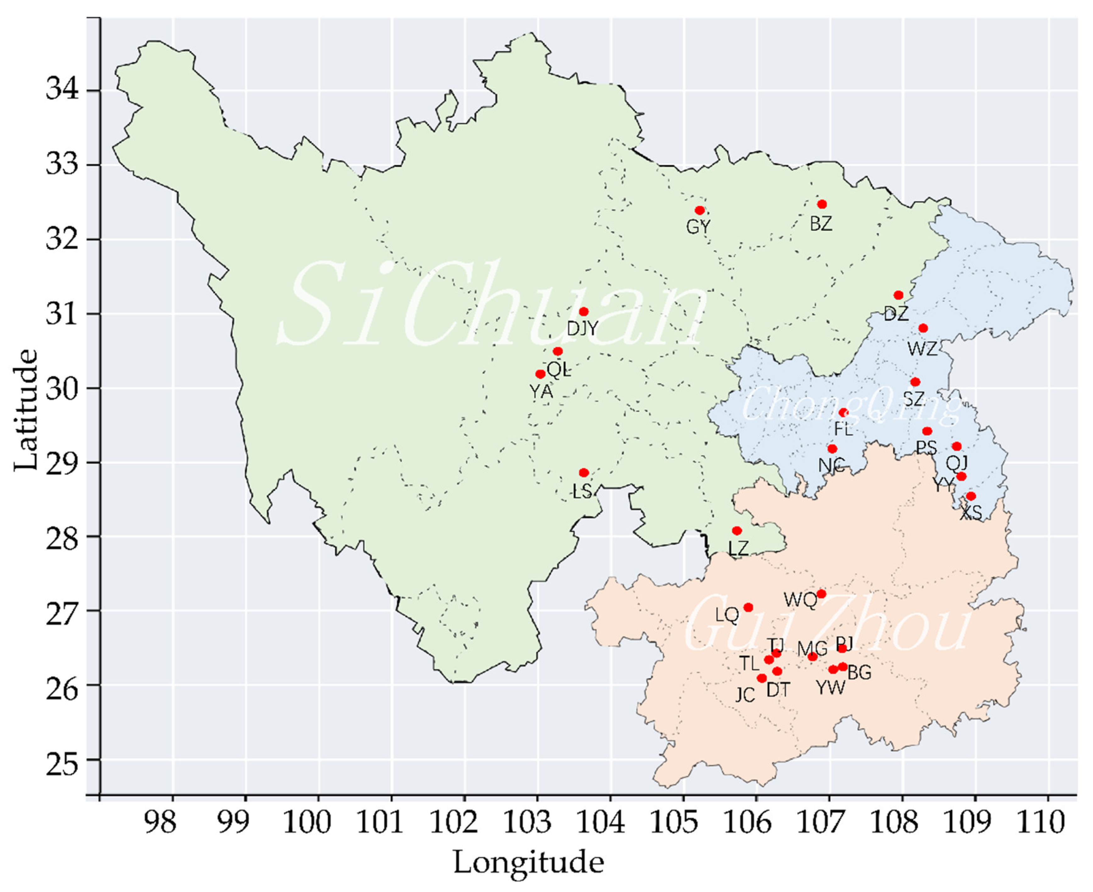
2.1. Sample Collection and DNA Extraction
2.2. PCR Amplification and Sequencing
2.3. Data Analysis
3. Result
3.1. Base Composition and Gene Mutation
3.2. Genetic Diversity
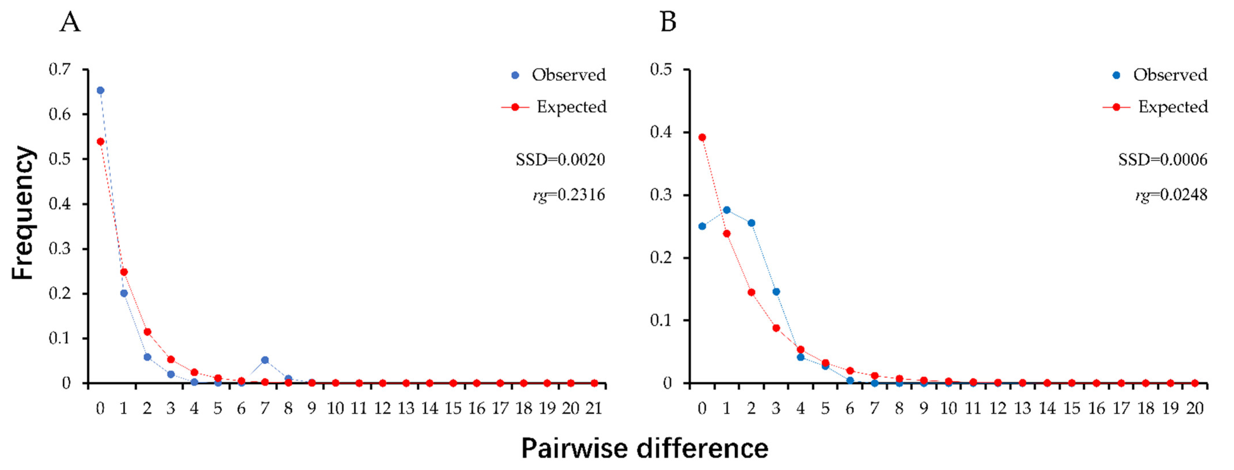
3.3. Population Demographic History
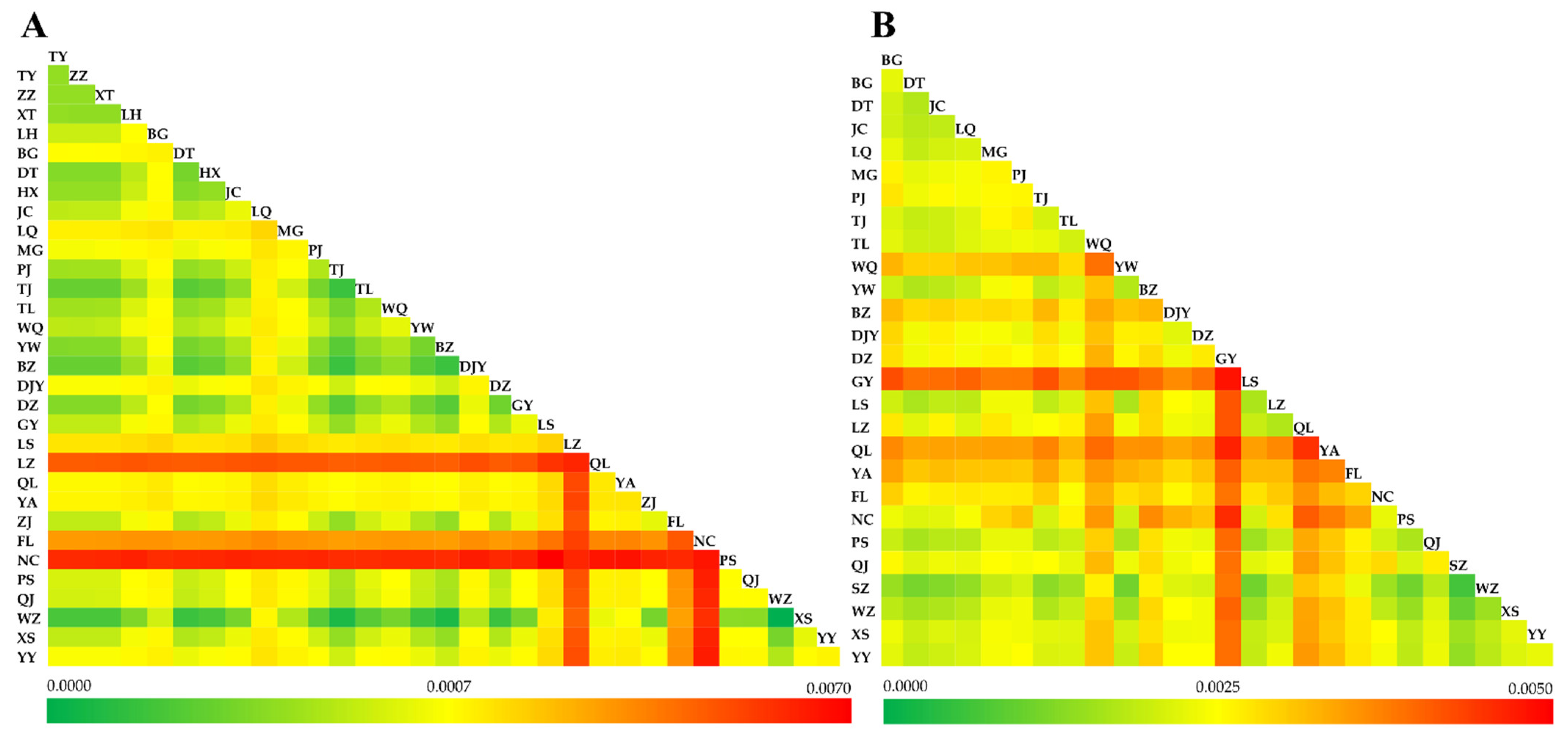
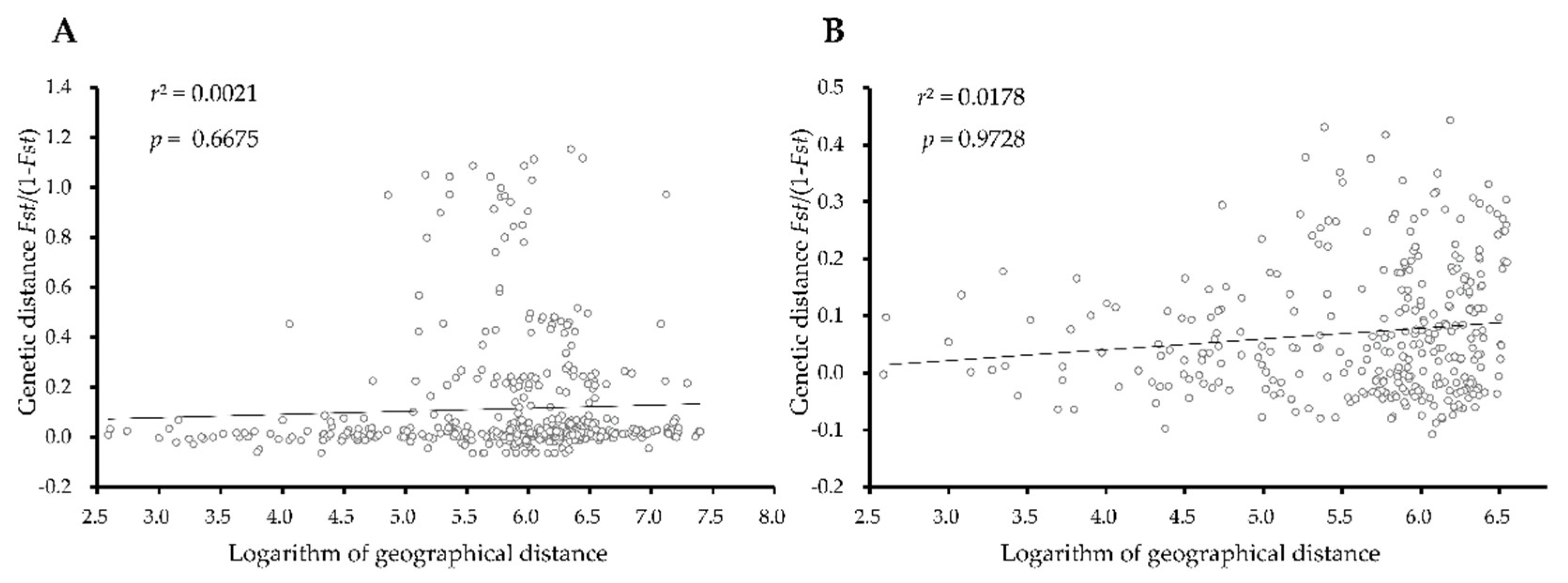
3.4. Genetic Differentiation
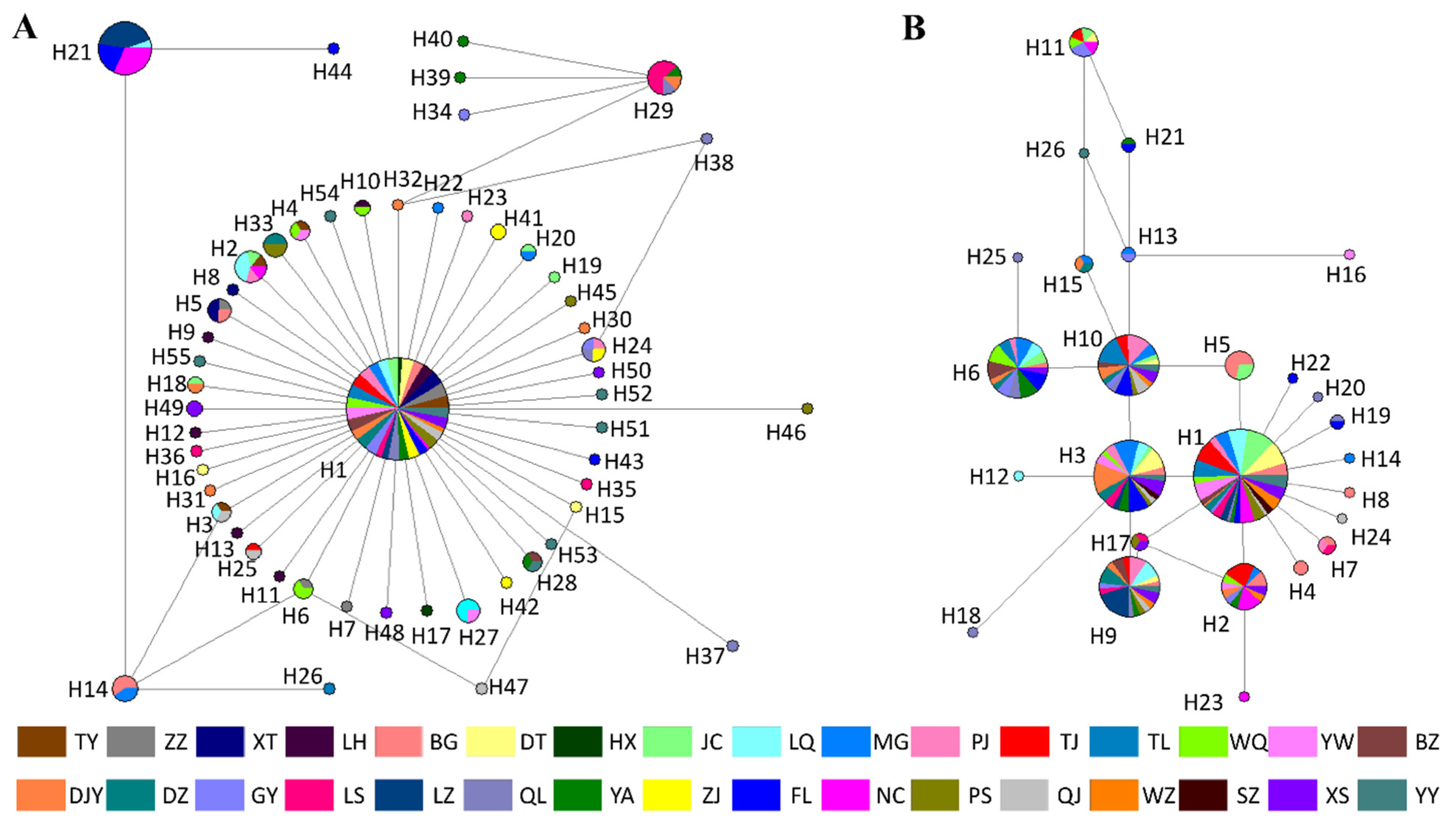
3.5. Haplotype Network Analysis
4. Discussion
5. Conclusions
Supplementary Materials
Author Contributions
Funding
Institutional Review Board Statement
Informed Consent Statement
Data Availability Statement
Acknowledgments
Conflicts of Interest
References
- Hughes, A.R.; Inouye, B.D.; Johnson, M.T.J.; Underwood, N.; Vellend, M. Ecological consequences of genetic diversity. Ecol. Lett. 2008, 11, 609–623. [Google Scholar] [CrossRef] [PubMed]
- Gienapp, P.; Teplitsky, C.; Alho, J.S.; Mills, J.A.; Meril, J. Climate change and evolution: Disentangling environmental and genetic responses. Mol. Ecol. 2008, 17, 167–178. [Google Scholar] [CrossRef] [PubMed]
- David, J.P.; Huber, K.; Failloux, A.B.; Rey, D.; Meyran, J.C. The role of environment in shaping the genetic diversity of the subalpine mosquito, Aedes rusticus (Diptera, Culicidae). Mol. Ecol. 2003, 12, 1951–1961. [Google Scholar] [CrossRef] [PubMed]
- Huang, S.; He, S.P.; Peng, Z.G.; Zhao, K.; Zhao, E.M. Molecular phylogeography of endangered sharp–snouted pitviper (Deinagkistrodon acutus; Reptilia, Viperidae) in Mainland China. Mol. Phylogenet. Evol. 2007, 44, 942–952. [Google Scholar] [CrossRef] [PubMed]
- Xun, H.Z.; Li, H.; Li, S.J.; Wei, S.J.; Zhang, L.J.; Song, F.; Jiang, P.; Yang, H.L.; Han, F.; Cai, W.Z. Population genetic structure and post–LGM expansion of the plant bug Nesidiocoris tenuis (Hemiptera: Miridae) in China. Sci. Rep. 2016, 6, 26755. [Google Scholar] [CrossRef] [PubMed] [Green Version]
- Terhorst, C.P.; Lau, J.A. Genetic variation in invasive species response to direct and indirect species interactions. Biol. Invasions 2014, 17, 651–659. [Google Scholar] [CrossRef]
- Zheng, S.Z.; Li, Y.; Yang, X.J.; Chen, J.Y.; Hua, J.; Gao, Y. DNA barcoding identification of Pseudococcidae (Hemiptera: Coccoidea) using the mitochondrial COI gene. Mitochondrial DNA B Resour. 2018, 3, 419–423. [Google Scholar] [CrossRef] [Green Version]
- Fang, Y.; Shi, W.Q.; Zhang, Y. Molecular phylogeny of Anopheles hyrcanus group members based on ITS2 rDNA. Parasit. Vectors 2017, 10, 417. [Google Scholar] [CrossRef] [Green Version]
- Cao, L.J.; Wang, Z.H.; Gong, Y.J.; Zhu, L.; Hoffmann, A.A.; Wei, S.J. Low genetic diversity but strong population structure reflects multiple introductions of western flower thrips (Thysanoptera: Thripidae) into China followed by human–mediated spread. Evol. Appl. 2017, 10, 391–401. [Google Scholar] [CrossRef] [Green Version]
- Rollins, L.A.; Woolnough, A.P.; Sinclair, R.; Mooney, N.J.; Sherwin, W.B. Mitochondrial DNA offers unique insights into invasion history of the common starling. Mol. Ecol. 2011, 20, 2307–2317. [Google Scholar] [CrossRef]
- Cameron, S.L. Insect mitochondrial genomics: Implications for evolution and phylogeny. Annu. Rev. Entomol. 2014, 59, 95–117. [Google Scholar] [CrossRef] [PubMed] [Green Version]
- Dickey, A.M.; Kumar, V.; Hoddle, M.S.; Funderburk, J.E.; Morgan, J.K.; Jara–Cavieres, A.; Shatters, R.G.J.; Osborne, L.S.; McKenzie, C.L. The scirtothrips dorsalis species complex: Endemism and invasion in a global pest. PLoS ONE 2015, 10, e0123747. [Google Scholar] [CrossRef] [PubMed] [Green Version]
- Tyagi, K.; Kumar, V.; Singha, D.; Chandra, K.; Laskar, B.A.; Kundu, S.; Chakraborty, R. DNA Barcoding studies on Thrips in India: Cryptic species and Species complexes. Sci. Rep. 2017, 7, 4898. [Google Scholar] [CrossRef] [Green Version]
- Vissing, J. Paternal comeback in mitochondrial DNA inheritance. Proc. Natl. Acad. Sci. USA 2019, 116, 1475–1476. [Google Scholar] [CrossRef] [PubMed] [Green Version]
- Dong, Z.K.; Wang, Y.Z.; Li, C.; Li, L.L. Mitochondrial DNA as a molecular marker in insect ecology: Current status and future prospects. Ann. Entomol. Soc. Am. 2021, 114, 470–476. [Google Scholar] [CrossRef]
- Triseleva, T.A.; Petrosyan, V.G.; Yatsuk, A.A.; Safonkin, A.F. Morphological and molecular (COI mtDNA) diversity of the polyzonal species of grass flies Meromyza Nigriseta Fedoseeva, 1960 (Diptera: Chloropidae). Acta. Zool. Bulg. 2020, 72, 339–346. [Google Scholar]
- Safonkina, A.F.; Triselevaa, T.A.; Yatsuka, A.A.; Petrosyan, V.G. Morphometric and Molecular Diversity of the Holarctic Meromyza saltatrix (L., 1761) (Diptera, Chloropidae) in Eurasia. Biol. Bull. Russ. Acad. Sci. 2018, 45, 310–319. [Google Scholar] [CrossRef]
- Palomares–Rius, J.E.; Cantalapiedra–Navarrete, C.; Archidona–Yuste, A.; Subbotin, S.A.; Castillo, P. The utility of mtDNA and rDNA for barcoding and phylogeny of plant–parasitic nematodes from Longidoridae (Nematoda, Enoplea). Sci. Rep. 2017, 7, 10905. [Google Scholar] [CrossRef] [Green Version]
- Cruz, D.O.; Jorge, D.M.M.; Pereira, J.O.P.; Torres, D.C.; Soares, C.E.A.; Freitas, B.M.; Grangeiro, T.B. Intraspecific variation in the first internal transcribed spacer (ITS1) of the nuclear ribosomal DNA in Melipona subnitida (Hymenoptera, Apidae), an endemic stingless bee from northeastern Brazil. Apidologie 2006, 37, 376–386. [Google Scholar] [CrossRef] [Green Version]
- Pereira, J.O.P.; Freitas, B.M.; Jorge, D.M.M.; Torres, D.C.; Soares, C.E.A.; Grangeiro, T.B. Genetic variability in Melipona quinquefasciata (Hymenoptera, Apidae, Meliponini) from northeastern Brazil determined using the first internal transcribed spacer (ITS1). Genet. Mol. Res. 2009, 8, 641–648. [Google Scholar] [CrossRef]
- Kapantaidaki, D.E.; Evangelou, V.I.; Morrison, W.R.; Leskey, T.C.; Brodeur, J.; Milonas, P. Halyomorpha halys (Hemiptera: Pentatomidae) Genetic Diversity in North America and Europe. Insects 2019, 10, 174. [Google Scholar] [CrossRef] [PubMed] [Green Version]
- Takeda, M. Genetic basis of photoperiodic control of summer and winter diapause in geographic ecotypes of the rice stem maggot, Chlorops oryzae. Entomol. Exp. Appl. 1998, 86, 59–70. [Google Scholar] [CrossRef]
- Takeda, M. Effects of photoperiod and temperature on larval development and summer diapause in two geographic ecotypes of the rice stem maggot, C. oryzae Matsumura (Diptera: Chloropidae). Appl. Entomol. Zool. 1997, 32, 63–74. [Google Scholar] [CrossRef] [Green Version]
- Takeda, M.; Nagata, T. Photoperiodic responses during larval development and diapause of two geographic ecotypes of the rice stem maggot, Chlorops oryzae. Entomol. Exp. Appl. 1992, 63, 273–281. [Google Scholar] [CrossRef]
- Wang, H.D.; Xu, Z.H.; Chen, Y.F.; Zhu, J.X.; Fang, Y.H. Rice yield loss due to Chlorops oryzae Matsumera and its action thresholds in rice fields in Zhejiang province. Zhi Wu Bao Hu 2007, 50, 383–388. [Google Scholar]
- Tian, P.; Qiu, L.; Zhou, A.L.; Chen, G.; He, H.L.; Ding, W.B.; Li, Y.Z. Evaluation of appropriate reference genes for investigating gene expression in C. oryzae (Diptera: Chloropidae). J. Econ. Entomol. 2019, 112, 2207–2214. [Google Scholar] [CrossRef]
- Tian, P.; Sun, H.M.; Chen, Y.K.; Li, X.W.; He, H.L.; Li, Y.Z. Occurrence and fungicides screening of the rice stem maggot Chlorops oryzae in Hunan Province. Zhi Wu Bao Hu Xue Bao 2021, 48, 388–395. [Google Scholar]
- Qiu, L.; Tao, S.J.; He, H.L.; Ding, W.B.; Li, Y.Z. Transcriptomics reveal the molecular underpinnings of chemosensory proteins in Chlorops oryzae. BMC Genom. 2018, 19, 890. [Google Scholar] [CrossRef]
- Wang, J.; Li, X.Y.; Du, R.B.; Liu, Y.H. The complete mitogenome of C. oryzae Matsumura (Diptera: Chloropidae). Mitochondrial DNA B Resour. 2021, 6, 1844–1846. [Google Scholar] [CrossRef]
- Zhou, A.L.; Tian, P.; Li, Z.C.; Li, X.W.; Tan, X.P.; Zhang, Z.B.; Qiu, L.; He, H.L.; Ding, W.B.; Li, Y.Z. Genetic diversity and differentiation of populations of C. oryzae (Diptera, Chloropidae). BMC Ecol. 2020, 20, 1–14. [Google Scholar] [CrossRef] [Green Version]
- De Barro, P.J.; Driver, F. Use of RAPD PCR to distinguish the B biotype from other biotypes of Bemisia tabaci (Gennadius) (Hemiptera: Aleyrodidae). Aust. J. Entomol. 1997, 36, 149–152. [Google Scholar] [CrossRef]
- Yu, Y.; Pham, N.; Xia, B.; Papusha, A.; Wang, G.; Yan, Z.; Peng, G.; Chen, K.; Ira, G. Dna2 nuclease deficiency results in large and complex DNA insertions at chromosomal breaks. Nature 2018, 564, 287–290. [Google Scholar] [CrossRef] [PubMed]
- Kumar, S.; Stecher, G.; Tamura, K. MEGA7: Molecular evolutionary genetics analysis version 7.0 for bigger datasets. Mol. Biol. Evol. 2016, 33, 1870–1874. [Google Scholar] [CrossRef] [PubMed] [Green Version]
- Librado, P.; Rozas, J. DnaSP v5: A software for comprehensive analysis of DNA polymorphism data. Bioinformatics 2009, 25, 1451–1452. [Google Scholar] [CrossRef] [Green Version]
- Fu, Y.X. Statistical tests of neutrality of mutations against population growth, hitchhiking and background selection. Genetics 1997, 147, 915–925. [Google Scholar] [CrossRef]
- Tajima, F. Statistical method for testing the neutral mutation hypothesis by DNA polymorphism. Genetics 1989, 123, 585–595. [Google Scholar] [CrossRef]
- Excoffier, L.; Lischer, H.E. Arlequin suite ver 3.5: A new series of programs to perform population genetics analyses under Linux and Windows. Mol. Ecol. Resour. 2010, 10, 564–567. [Google Scholar] [CrossRef]
- Kantharaja, D.C.; Lakkundi, T.K.; Basavanna, M.; Manjappa, S. Spatial analysis of fluoride concentration in groundwaters of Shivani watershed area, Karnataka state, South India, through geospatial information system. Environ. Earth. Sci. 2012, 65, 67–76. [Google Scholar] [CrossRef]
- Rohlf, F.J. NTSYS–pc, Numerical Taxonomy and Multivariate Analysis System, version 2.1e; Exeter Software: Setauket, NY, USA, 2000. [Google Scholar]
- Polzin, T.; Daneshmand, S.V. On Steiner trees and minimum spanning trees in hypergraphs. Oper. Res. Lett. 2003, 31, 12–20. [Google Scholar] [CrossRef]
- Amos, W.; Harwood, J. Factors affecting levels of genetic diversity in natural populations. Philos. Trans. R. Soc. Lond. B Biol. Sci. 1998, 353, 177–186. [Google Scholar] [CrossRef] [Green Version]
- Avise, J.C. Perspective: Conservation genetics enters the genomics era. Conserv. Genet. 2010, 11, 665–669. [Google Scholar] [CrossRef] [Green Version]
- Toews, D.P.L.; Brelsford, A. The biogeography of mitochondrial and nuclear discordance in animals. Mol. Ecol. 2012, 21, 3907–3930. [Google Scholar] [CrossRef] [PubMed]
- Fontaine, M.C.; Snirc, A.; Frantzis, A.; Koutrakis, E.; Ozturk, B.; Ozturk, A.A.; Austerlitz, F. History of expansion and anthropogenic collapse in a top marine predator of the Black Sea estimated from genetic data. Proc. Natl. Acad. Sci. USA 2012, 109, E2569–E2576. [Google Scholar] [CrossRef] [PubMed] [Green Version]
- Liao, J.C.; Jing, D.D.; Luo, G.J.; Wang, Y.; Zhao, L.M.; Liu, N.F. Comparative phylogeography of Meriones meridianus, Dipus sagitta, and Allactaga sibirica: Potential indicators of the impact of the Qinghai–Tibetan Plateau uplift. Mamm. Biol. 2016, 81, 31–39. [Google Scholar] [CrossRef]
- Cristiano, M.P.; Clemes Cardoso, D.; Fernandes–Salomão, T.M.; Heinze, J. Integrating paleodistribution models and phylogeography in the Grass–Cutting Ant Acromyrmex striatus (Hymenoptera: Formicidae) in southern lowlands of south America. PLoS ONE 2016, 11, e0146734. [Google Scholar] [CrossRef]
- Vinas, J.; Bremer, J.A.; Pla, C. Phylogeography of the Atlantic bonito (Sarda sarda) in the northern Mediterranean: The combined effects of historical vicariance, population expansion, secondary invasion, and isolation by distance. Mol. Phylogenet. Evol. 2004, 33, 32–42. [Google Scholar] [CrossRef]
- Zhang, F.M.; Ge, S. Data analysis in population genetics. I. analysis of RAPD data with AMOVA. Sheng Wu Duo Yang Xing 2002, 10, 438–444. [Google Scholar]
- Rousset, F. Genetic differentiation and estimation of gene flow from F–Statistics under isolation by distance. Genetics 1997, 145, 1219–1228. [Google Scholar] [CrossRef]
- Miller, N.J.; Birley, A.J.; Overall, A.D.J.; Tatchell1, G.M. Population genetic structure of the lettuce root aphid, Pemphigus bursarius (L.), in relation to geographic distance, gene flow and host plant usage. Heredity 2003, 91, 217–223. [Google Scholar] [CrossRef]
- Slatkin, M. Gene flow and the geographic structure of natural populations. Science 1987, 236, 787–792. [Google Scholar] [CrossRef]
- Fuentes–Contreras, E.; Basoalto, E.; Franck, P.; Lavandero, B.; Knight, A.L.; Ramirez, C.C. Measuring local genetic variability in populations of codling moth (Lepidoptera: Tortricidae) across an unmanaged and commercial orchard interface. Environ. Entomol. 2014, 43, 520–527. [Google Scholar] [CrossRef] [PubMed]
- Xu, Y.; Mai, J.W.; Yu, B.J.; Hu, H.X.; Yuan, L.; Jashenko, R.; Ji, R. Study on the genetic differentiation of geographic populations of Calliptamus italicus (Orthoptera: Acrididae) in sino–kazakh border areas based on mitochondrial COI and COII genes. J. Econ. Entomol. 2019, 112, 1912–1919. [Google Scholar] [CrossRef] [PubMed]
- Nei, M.; Maruyama, T.; Chakraborty, R. The bottleneck effect and genetic variability in populations. Evolution 1975, 29, 1–10. [Google Scholar] [CrossRef] [PubMed]


| n | h | k | Hd | Pi | Tajima’s D | Fu’ Fs | |
|---|---|---|---|---|---|---|---|
| TY | 24 | 4 | 0.250 | 0.239 ± 0.113 | 0.0004 ± 0.0002 | −1.7325 ** | −3.0208 *** |
| ZZ | 24 | 4 | 0.250 | 0.239 ± 0.113 | 0.0004 ± 0.0002 | −1.7325 | −3.0208 *** |
| XT | 24 | 3 | 0.243 | 0.236 ± 0.109 | 0.0003 ± 0.0002 | −1.2023 * | −1.4074 ** |
| LH | 23 | 6 | 0.435 | 0.395 ± 0.128 | 0.0006 ± 0.0002 | −1.9921 *** | −4.8874 *** |
| BG | 20 | 3 | 0.637 | 0.353 ± 0.123 | 0.0009 ± 0.0003 | −0.6594 | 0.2535 |
| DT | 20 | 3 | 0.200 | 0.195 ± 0.115 | 0.0003 ± 0.0002 | −1.5128 ** | −1.8631 ** |
| HX | 8 | 2 | 0.250 | 0.250 ± 0.180 | 0.0004 ± 0.0003 | −1.0548 | −0.1820 |
| JC | 20 | 5 | 0.400 | 0.368 ± 0.135 | 0.0006 ± 0.0002 | −1.8679 ** | −3.6541 *** |
| LQ | 20 | 4 | 1.058 | 0.432 ± 0.126 | 0.0015 ± 0.0008 | −1.7892 ** | 0.1219 |
| MG | 20 | 4 | 0.579 | 0.363 ± 0.131 | 0.0008 ± 0.0003 | −1.4084 * | −1.2369 * |
| PJ | 20 | 4 | 0.300 | 0.284 ± 0.128 | 0.0004 ± 0.0002 | −1.7233 ** | −2.7493 *** |
| TJ | 20 | 2 | 0.100 | 0.100 ± 0.088 | 0.0001 ± 0.0001 | −1.1644 | −0.8793 * |
| TL | 20 | 2 | 0.300 | 0.100 ± 0.088 | 0.0004 ± 0.0004 | −1.7233 ** | 0.5439 |
| WQ | 20 | 4 | 0.389 | 0.363 ± 0.131 | 0.0005 ± 0.0002 | −1.4407 * | −2.1353 *** |
| YW | 20 | 3 | 0.200 | 0.195 ± 0.115 | 0.0003 ± 0.0002 | −1.5128 ** | −1.8631 ** |
| BZ | 20 | 2 | 0.100 | 0.100 ± 0.088 | 0.0001 ± 0.0001 | −1.1644 | −0.8793 * |
| DJY | 20 | 6 | 0.589 | 0.447 ± 0.137 | 0.0008 ± 0.0003 | −1.7800 ** | −4.0149 *** |
| DZ | 20 | 2 | 0.189 | 0.189 ± 0.108 | 0.0003 ± 0.0002 | −0.5916 | −0.0966 |
| GY | 20 | 3 | 0.400 | 0.195 ± 0.115 | 0.0006 ± 0.0004 | −1.8679 *** | −0.6256 |
| LS | 17 | 4 | 1.118 | 0.596 ± 0.099 | 0.0016 ± 0.0003 | −0.1695 | 0.0627 |
| LZ | 21 | 3 | 3.724 | 0.638 ± 0.058 | 0.0052 ± 0.0006 | 2.2431 | 6.1273 |
| QL | 20 | 5 | 0.779 | 0.368 ± 0.135 | 0.0011 ± 0.0005 | −1.7190 ** | −1.7642 ** |
| YA | 20 | 5 | 0.837 | 0.368 ± 0.135 | 0.0012 ± 0.0005 | −1.2429 | −1.5755 * |
| ZJ | 20 | 4 | 0.389 | 0.363 ± 0.131 | 0.0005 ± 0.0002 | −1.4407 * | −2.1353 *** |
| FL | 20 | 4 | 2.963 | 0.489 ± 0.117 | 0.0041 ± 0.0010 | 0.5779 | 3.1379 |
| NC | 12 | 3 | 3.985 | 0.621 ± 0.087 | 0.0055 ± 0.0006 | 2.0135 | 4.6229 |
| PS | 21 | 4 | 0.467 | 0.348 ± 0.128 | 0.0007 ± 0.0003 | −1.6536 ** | −1.6755 ** |
| QJ | 17 | 4 | 0.471 | 0.331 ± 0.143 | 0.0007 ± 0.0003 | −1.8431 ** | −1.8636 ** |
| WZ | 7 | 1 | 0.000 | 0.000 ± 0.000 | 0.0000 ± 0.0000 | N | N |
| XS | 20 | 4 | 0.389 | 0.363 ± 0.131 | 0.0005 ± 0.0002 | −1.4407 * | −2.1353 ** |
| YY | 20 | 7 | 0.600 | 0.521 ± 0.135 | 0.0008 ± 0.0003 | −2.0562 *** | −5.6554 *** |
| Total | 598 | 55 | 0.854 | 0.346 ± 0.026 | 0.0012 ± 0.0001 | −2.4784 *** | −3.40 × 1038 *** |
| n | h | k | Hd | Pi | Tajima’s D | Fu’ Fs | |
|---|---|---|---|---|---|---|---|
| BG | 23 | 9 | 1.375 | 0.838 ± 0.056 | 0.0023 ± 0.0004 | −0.8686 | −4.5472 *** |
| DT | 20 | 5 | 1.068 | 0.558 ± 0.114 | 0.0018 ± 0.0006 | −1.1736 | −0.9454 |
| JC | 24 | 6 | 1.145 | 0.500 ± 0.121 | 0.0019 ± 0.0006 | −0.8693 | −1.5615 |
| LQ | 19 | 8 | 1.298 | 0.649 ± 0.108 | 0.0021 ± 0.0005 | −0.2877 | −0.5202 |
| MG | 22 | 8 | 1.576 | 0.818 ± 0.059 | 0.0026 ± 0.0004 | −0.1321 | −2.8304 ** |
| PJ | 15 | 6 | 1.562 | 0.848 ± 0.054 | 0.0026 ± 0.0003 | 0.0531 | −1.4952 |
| TJ | 21 | 5 | 1.267 | 0.595 ± 0.108 | 0.0021 ± 0.0007 | −0.7553 | −0.4465 |
| TL | 17 | 3 | 1.250 | 0.588 ± 0.093 | 0.0021 ± 0.0003 | 1.1573 | 1.5858 |
| WQ | 10 | 5 | 2.356 | 0.800 ± 0.100 | 0.0039 ± 0.0009 | −0.2034 | −0.2303 |
| YW | 14 | 4 | 1.077 | 0.495 ± 0.151 | 0.0018 ± 0.0009 | −1.5407 ** | −0.2586 |
| BZ | 9 | 4 | 1.944 | 0.806 ± 0.089 | 0.0032 ± 0.0004 | 1.3055 | 0.3315 |
| DJY | 13 | 7 | 1.346 | 0.795 ± 0.109 | 0.0022 ± 0.0005 | −0.5866 | −3.6278 *** |
| DZ | 12 | 6 | 1.636 | 0.848 ± 0.074 | 0.0027 ± 0.0004 | −0.0430 | −1.8724 * |
| GY | 10 | 7 | 2.911 | 0.933 ± 0.062 | 0.0048 ± 0.0006 | 0.7476 | −2.1342 * |
| LS | 10 | 5 | 1.022 | 0.756 ± 0.130 | 0.0017 ± 0.0004 | −0.1297 | −2.2036 ** |
| LZ | 11 | 3 | 1.055 | 0.618 ± 0.104 | 0.0017 ± 0.0003 | 1.6648 | 0.6938 |
| QL | 10 | 8 | 2.733 | 0.956 ± 0.059 | 0.0045 ± 0.0006 | −0.6167 | −3.8821 *** |
| YA | 10 | 6 | 2.244 | 0.889 ± 0.075 | 0.0037 ± 0.0006 | 0.2410 | −1.5332 |
| FL | 17 | 7 | 1.779 | 0.868 ± 0.045 | 0.0029 ± 0.0005 | −0.4858 | −1.9303 * |
| NC | 13 | 4 | 1.385 | 0.603 ± 0.131 | 0.0023 ± 0.0010 | −1.4646 * | 0.1989 |
| PS | 10 | 5 | 1.022 | 0.667 ± 0.163 | 0.0017 ± 0.0005 | −0.1297 | −2.2036 ** |
| QJ | 7 | 5 | 1.619 | 0.905 ± 0.103 | 0.0027 ± 0.0005 | −0.0398 | −2.0192 ** |
| SZ | 5 | 2 | 0.400 | 0.400 ± 0.237 | 0.0007 ± 0.0004 | −0.8165 | 0.0902 |
| WZ | 10 | 4 | 0.933 | 0.533 ± 0.180 | 0.0015 ± 0.0006 | −0.4313 | −1.0204 |
| XS | 17 | 7 | 1.360 | 0.809 ± 0.079 | 0.0022 ± 0.0004 | 0.4581 | −2.8195 ** |
| YY | 11 | 5 | 1.382 | 0.618 ± 0.164 | 0.0023 ± 0.0008 | −0.7301 | −1.2656 * |
| Total | 360 | 26 | 1.551 | 0.750 ± 0.021 | 0.0026 ± 0.0001 | −1.2621 * | −16.0072 *** |
| Source of Variation | d.f. | SS | Variance Components | % | F-Statistic | |
|---|---|---|---|---|---|---|
| COI | Among populations | 30 | 56.336 | 0.079 Va ** | 18.32 | |
| Within populations | 567 | 200.070 | 0.353 Vb ** | 81.68 | ||
| Total | 597 | 256.406 | 0.432 | 100.00 | Fst = 0.183 ** | |
| ITS1 | Among populations | 25 | 35.596 | 0.050 Va ** | 6.47 | |
| Within populations | 334 | 243.645 | 0.727 Vb ** | 93.53 | ||
| Total | 359 | 278.383 | 0.777 | 100.00 | Fst = 0.065 ** |
| TY | ZZ | XT | LH | BG | DT | HX | JC | LQ | MG | PJ | TJ | TL | WQ | YW | BZ | DJY | DZ | GY | LS | LZ | QL | YA | ZJ | FL | NC | PS | QJ | WZ | XS | YY | |
|---|---|---|---|---|---|---|---|---|---|---|---|---|---|---|---|---|---|---|---|---|---|---|---|---|---|---|---|---|---|---|---|
| TY | hun | 33.84 | hun | 84.97 | 55.43 | inf | inf | inf | 91.75 | inf | 10.23 | hun | inf | inf | 7.53 | 19.07 | 1.01 | 1.96 | hun | 22.24 | inf | 30.04 | 26.64 | 2.05 | 0.45 | 32.27 | inf | 26.63 | hun | inf | |
| ZZ | 0.00 | inf | hun | 15.20 | 55.43 | hun | inf | inf | inf | inf | 12.80 | hun | inf | hun | 7.53 | 19.07 | 1.01 | 1.96 | hun | 22.24 | inf | 30.04 | 26.64 | 2.05 | 0.45 | 32.27 | inf | 26.63 | hun | inf | |
| XT | 0.01 | 0.00 | 44.14 | 10.88 | 12.64 | 34.56 | 34.44 | 29.49 | 16.21 | 32.31 | 7.35 | 30.81 | 32.31 | 36.43 | 6.75 | 14.72 | 0.97 | 1.90 | 36.24 | 12.62 | 29.49 | 19.26 | 16.21 | 1.92 | 0.43 | 19.09 | inf | 16.21 | 39.34 | 29.77 | |
| LH | 0.00 | 0.00 | 0.01 | 15.60 | 22.66 | inf | inf | inf | hun | inf | 8.16 | inf | inf | inf | 9.38 | 25.23 | 1.05 | 2.37 | inf | 36.24 | inf | 43.51 | 40.25 | 2.12 | 0.49 | 46.32 | inf | 40.25 | hun | hun | |
| BG | 0.01 | 0.03 | 0.04 | 0.03 | hun | 56.06 | 57.78 | 13.85 | 22.34 | 14.99 | 57.04 | inf | 14.99 | 59.38 | 8.94 | 14.43 | 1.84 | 3.22 | 17.26 | 11.92 | 13.85 | 15.57 | 13.73 | 5.29 | 0.86 | 14.20 | inf | 13.74 | 19.57 | hun | |
| DT | 0.01 | 0.01 | 0.04 | 0.02 | 0.00 | 20.81 | inf | 16.16 | inf | 18.48 | inf | inf | 18.48 | 43.79 | 8.35 | 15.99 | 1.37 | 2.57 | 23.07 | 12.18 | 16.16 | 18.38 | 15.27 | 3.17 | 0.63 | 16.83 | inf | 15.28 | 27.80 | inf | |
| HX | 0.00 | 0.00 | 0.01 | 0.00 | 0.01 | 0.02 | hun | hun | 32.59 | hun | 7.40 | inf | hun | inf | 8.96 | hun | 1.09 | 2.23 | inf | 23.21 | hun | 42.20 | hun | 2.21 | 0.50 | 42.09 | inf | 32.59 | inf | hun | |
| JC | 0.00 | 0.00 | 0.01 | 0.00 | 0.01 | 0.00 | 0.00 | hun | inf | hun | hun | inf | hun | hun | 8.96 | 25.49 | 1.19 | 2.23 | hun | 23.17 | hun | 42.09 | 32.57 | 2.56 | 0.53 | 41.98 | inf | 32.53 | hun | inf | |
| LQ | 0.00 | 0.00 | 0.02 | 0.00 | 0.03 | 0.03 | 0.00 | 0.00 | 23.25 | hun | 5.83 | 11.98 | hun | inf | 7.41 | 20.92 | 1.04 | 1.86 | hun | 13.73 | hun | 33.01 | 23.29 | 2.08 | 0.46 | 33.47 | inf | 23.25 | inf | inf | |
| MG | 0.01 | 0.00 | 0.03 | 0.00 | 0.02 | 0.00 | 0.02 | 0.00 | 0.02 | hun | 37.44 | inf | 27.93 | 37.32 | 8.28 | 18.40 | 1.20 | 2.32 | 37.18 | 13.75 | 23.25 | 23.17 | 18.44 | 2.59 | 0.55 | 21.53 | inf | 18.43 | 46.85 | inf | |
| PJ | 0.00 | 0.00 | 0.02 | 0.00 | 0.03 | 0.03 | 0.00 | 0.00 | 0.00 | 0.00 | 6.61 | 54.09 | hun | hun | 8.18 | 23.20 | 1.08 | 2.05 | hun | 18.48 | hun | 37.55 | 27.94 | 2.14 | 0.48 | 37.87 | inf | 27.93 | inf | hun | |
| TJ | 0.05 | 0.04 | 0.06 | 0.06 | 0.01 | 0.00 | 0.06 | 0.00 | 0.08 | 0.01 | 0.07 | 16.06 | 6.61 | 8.18 | 5.80 | 8.36 | 1.49 | 2.36 | 8.18 | 5.61 | 5.83 | 8.28 | 6.94 | 3.60 | 0.67 | 7.49 | hun | 6.94 | 9.74 | inf | |
| TL | 0.00 | 0.00 | 0.02 | 0.00 | 0.00 | 0.00 | 0.00 | 0.00 | 0.04 | 0.00 | 0.01 | 0.03 | 54.09 | inf | 38.44 | inf | 1.75 | 3.64 | inf | 13.47 | 11.98 | inf | inf | 4.24 | 0.84 | inf | inf | inf | inf | inf | |
| WQ | 0.00 | 0.00 | 0.02 | 0.00 | 0.03 | 0.03 | 0.00 | 0.00 | 0.00 | 0.02 | 0.00 | 0.07 | 0.01 | hun | 9.73 | 23.20 | 1.06 | 2.05 | hun | 18.48 | hun | 37.55 | 27.94 | 2.14 | 0.48 | 37.87 | inf | 27.93 | inf | inf | |
| YW | 0.00 | 0.00 | 0.01 | 0.00 | 0.01 | 0.01 | 0.00 | 0.00 | 0.00 | 0.01 | 0.00 | 0.06 | 0.00 | 0.00 | 9.73 | 27.75 | 1.11 | 2.42 | hun | 28.10 | inf | hun | 37.29 | 2.27 | 0.52 | 46.14 | inf | 37.32 | hun | hun | |
| BZ | 0.06 | 0.06 | 0.07 | 0.05 | 0.05 | 0.06 | 0.05 | 0.05 | 0.06 | 0.06 | 0.06 | 0.08 | 0.01 | 0.05 | 0.05 | inf | 1.18 | hun | hun | 6.96 | 8.80 | inf | 8.28 | 2.36 | 0.59 | 8.75 | inf | 8.28 | 13.39 | 13.83 | |
| DJY | 0.03 | 0.03 | 0.03 | 0.02 | 0.03 | 0.03 | 0.00 | 0.02 | 0.02 | 0.03 | 0.02 | 0.06 | 0.00 | 0.02 | 0.02 | 0.00 | 1.20 | 6.58 | inf | 15.35 | 20.92 | inf | 49.90 | 2.46 | 0.59 | 19.63 | inf | 18.40 | 32.35 | 34.49 | |
| DZ | 0.33 * | 0.33 * | 0.34 * | 0.32 * | 0.21 | 0.27 | 0.31 | 0.30 | 0.32 | 0.29 | 0.32 | 0.25 | 0.22 | 0.32 | 0.31 | 0.30 | 0.29 | 1.18 | 1.11 | 1.06 | 1.04 | 1.16 | 1.11 | inf | inf | 1.10 | 1.88 | 1.11 | 1.16 | 1.36 | |
| GY | 0.20 | 0.20 | 0.21 | 0.17 | 0.13 | 0.16 | 0.18 | 0.18 | 0.21 | 0.18 | 0.20 | 0.17 | 0.12 | 0.20 | 0.17 | 0.00 | 0.07 | 0.30 * | 3.99 | 1.96 | 1.86 | 6.24 | 2.32 | 2.08 | 0.64 | 2.43 | 4.16 | 2.32 | 2.79 | 2.70 | |
| LS | 0.00 | 0.00 | 0.01 | 0.00 | 0.03 | 0.02 | 0.00 | 0.00 | 0.00 | 0.01 | 0.00 | 0.06 | 0.00 | 0.00 | 0.00 | 0.00 | 0.00 | 0.31 | 0.11 | 28.02 | hun | inf | hun | 2.28 | 0.52 | 45.97 | inf | 37.18 | hun | hun | |
| LZ | 0.02 | 0.02 | 0.04 | 0.01 | 0.04 | 0.04 | 0.02 | 0.02 | 0.04 | 0.04 | 0.03 | 0.08 | 0.04 | 0.03 | 0.02 | 0.07 | 0.03 | 0.32 | 0.20 | 0.02 | 13.73 | 18.58 | 13.77 | 2.11 | 0.48 | inf | inf | 13.75 | 37.84 | 24.40 | |
| QL | 0.00 | 0.00 | 0.02 | 0.00 | 0.03 | 0.03 | 0.00 | 0.00 | 0.00 | 0.02 | 0.00 | 0.08 | 0.04 | 0.00 | 0.00 | 0.05 | 0.02 | 0.32 | 0.21 | 0.00 | 0.04 | 33.01 | 23.29 | 2.08 | 0.46 | 33.47 | inf | 23.25 | inf | 80.93 | |
| YA | 0.02 | 0.02 | 0.03 | 0.01 | 0.03 | 0.03 | 0.01 | 0.01 | 0.01 | 0.02 | 0.01 | 0.06 | 0.00 | 0.01 | 0.00 | 0.00 | 0.00 | 0.30 | 0.07 | 0.00 | 0.03 | 0.01 | 23.15 | 2.37 | 0.55 | 25.77 | inf | 23.17 | 55.93 | 55.93 | |
| ZJ | 0.02 | 0.02 | 0.03 | 0.01 | 0.04 | 0.03 | 0.00 | 0.02 | 0.02 | 0.03 | 0.02 | 0.07 | 0.00 | 0.02 | 0.01 | 0.06 | 0.01 | 0.31 | 0.18 | 0.00 | 0.04 | 0.02 | 0.02 | 2.24 | 0.51 | 21.54 | inf | 18.44 | 46.80 | 37.58 | |
| FL | 0.20 | 0.20 | 0.21 | 0.19 | 0.09 | 0.14 | 0.18 | 0.16 | 0.19 | 0.16 | 0.19 | 0.12 | 0.11 | 0.19 | 0.18 | 0.17 | 0.17 | 0.00 | 0.19 | 0.18 | 0.19 | 0.19 | 0.17 | 0.18 | 7.37 | 2.23 | 5.00 | 2.24 | 2.41 | 3.05 | |
| NC | 0.53 | 0.53 * | 0.54 * | 0.51 * | 0.37 | 0.44 * | 0.50 * | 0.48 | 0.52 | 0.48 | 0.51 | 0.43 * | 0.37 | 0.51 * | 0.49 | 0.46 * | 0.46 * | 0.00 | 0.44 * | 0.49 * | 0.51 * | 0.52 | 0.47 | 0.49 * | 0.06 | 0.52 | 0.88 | 0.51 | 0.56 | 0.63 | |
| PS | 0.02 | 0.02 | 0.03 | 0.01 | 0.03 | 0.03 | 0.01 | 0.01 | 0.01 | 0.02 | 0.01 | 0.06 | 0.00 | 0.01 | 0.01 | 0.05 | 0.02 | 0.31 | 0.17 | 0.01 | 0.00 | 0.01 | 0.02 | 0.02 | 0.18 | 0.49 | inf | 21.53 | 53.73 | 48.57 | |
| QJ | 0.00 | 0.00 | 0.00 | 0.00 | 0.00 | 0.00 | 0.00 | 0.00 | 0.00 | 0.00 | 0.00 | 0.00 | 0.00 | 0.00 | 0.00 | 0.00 | 0.00 | 0.21 | 0.11 | 0.00 | 0.00 | 0.00 | 0.00 | 0.00 | 0.09 | 0.36 | 0.00 | inf | inf | inf | |
| WZ | 0.02 | 0.02 | 0.03 | 0.01 | 0.04 | 0.03 | 0.02 | 0.02 | 0.02 | 0.03 | 0.02 | 0.07 | 0.00 | 0.02 | 0.01 | 0.06 | 0.03 | 0.31 * | 0.18 | 0.01 | 0.04 | 0.02 | 0.02 | 0.03 | 0.18 | 0.49 | 0.02 | 0.00 | 46.85 | 37.64 | |
| XS | 0.00 | 0.00 | 0.01 | 0.00 | 0.02 | 0.02 | 0.00 | 0.00 | 0.00 | 0.01 | 0.00 | 0.05 | 0.00 | 0.00 | 0.00 | 0.04 | 0.02 | 0.30 * | 0.15 | 0.00 | 0.01 | 0.00 | 0.01 | 0.01 | 0.17 | 0.47 | 0.01 | 0.00 | 0.01 | inf | |
| YY | 0.00 | 0.00 | 0.02 | 0.00 | 0.00 | 0.00 | 0.00 | 0.00 | 0.00 | 0.00 | 0.00 | 0.00 | 0.00 | 0.00 | 0.00 | 0.03 | 0.01 | 0.27 | 0.16 | 0.00 | 0.02 | 0.01 | 0.01 | 0.01 | 0.14 | 0.44 | 0.01 | 0.00 | 0.01 | 0.00 |
| BG | DT | JC | LQ | MG | PJ | TJ | TL | WQ | YW | BZ | DJY | DZ | GY | LS | LZ | QL | YA | FL | PS | NC | QJ | SZ | WZ | XS | YY | |
|---|---|---|---|---|---|---|---|---|---|---|---|---|---|---|---|---|---|---|---|---|---|---|---|---|---|---|
| BG | 11.41 | inf | 6.74 | 3.29 | 1.83 | inf | 7.89 | 3.58 | inf | 1.37 | 0.87 | 1.80 | 0.96 | 12.38 | 0.75 | 2.23 | 1.45 | 1.72 | inf | 9.08 | 5.23 | inf | inf | 6.63 | inf | |
| DT | 0.02 | hun | inf | 7.09 | 2.69 | 49.45 | 4.64 | 3.49 | inf | 1.28 | 1.25 | 3.52 | 1.01 | inf | 0.99 | 2.21 | 1.65 | 2.28 | inf | 3.34 | 76.44 | inf | inf | inf | inf | |
| JC | 0.00 | 0.00 | 7.13 | 4.94 | 1.66 | 23.47 | 21.04 | 5.36 | inf | 1.29 | 0.84 | 1.66 | 1.01 | 5.09 | 0.58 | 2.28 | 1.48 | 2.12 | 61.78 | 3.58 | 4.37 | inf | inf | 4.90 | inf | |
| LQ | 0.04 | 0.00 | 0.03 | 15.24 | 9.22 | 8.34 | 6.28 | 7.23 | 17.70 | 3.35 | 2.17 | hun | 1.23 | inf | 2.25 | 5.77 | 3.67 | 3.57 | inf | 2.36 | inf | inf | inf | inf | inf | |
| MG | 0.07 | 0.03 | 0.05 | 0.02 | inf | 2.49 | inf | inf | 2.71 | inf | 26.09 | inf | 5.00 | 2.68 | 1.11 | inf | inf | inf | 5.22 | 1.32 | inf | 4.27 | 3.04 | inf | inf | |
| PJ | 0.12 | 0.09 | 0.13 | 0.03 | 0.00 | 1.51 | 11.42 | inf | 1.41 | inf | inf | inf | 5.20 | 2.43 | 2.52 | inf | inf | inf | 3.96 | 0.90 | inf | 1.60 | 1.81 | inf | inf | |
| TJ | 0.00 | 0.01 | 0.01 | 0.03 | 0.09 | 0.14 | 2.57 | 2.56 | inf | 1.03 | 0.81 | 1.76 | 0.90 | inf | 0.90 | 1.52 | 1.25 | 1.29 | inf | inf | 3.69 | inf | inf | 8.81 | inf | |
| TL | 0.03 | 0.05 | 0.01 | 0.04 | 0.00 | 0.02 | 0.09 | inf | 2.61 | 10.31 | 2.35 | 5.70 | 2.59 | 1.90 | 0.66 | inf | 10.47 | inf | 4.11 | 1.22 | inf | 3.05 | 2.96 | 10.68 | inf | |
| WQ | 0.07 | 0.07 | 0.04 | 0.03 | 0.00 | 0.00 | 0.09 | 0.00 | 2.30 | inf | 9.79 | inf | inf | 2.20 | 1.06 | inf | inf | inf | 3.79 | 1.70 | inf | 3.76 | 2.82 | 15.20 | inf | |
| YW | 0.00 | 0.00 | 0.00 | 0.01 | 0.08 | 0.16 | 0.00 | 0.09 | 0.10 | 0.93 | 0.76 | 1.57 | 0.82 | inf | 0.71 | 1.63 | 1.16 | 1.39 | inf | 26.12 | 3.46 | inf | inf | 7.00 | inf | |
| BZ | 0.15 | 0.16 | 0.16 | 0.07 | 0.00 | 0.00 | 0.19 | 0.02 | 0.00 | 0.21 | inf | inf | inf | 1.21 | 1.35 | inf | inf | inf | 1.72 | 0.74 | inf | 1.01 | 1.13 | 6.88 | 2.90 | |
| DJY | 0.22 | 0.17 | 0.23 | 0.10 | 0.01 | 0.00 | 0.23 | 0.10 | 0.02 | 0.25 | 0.00 | inf | 5.61 | 0.94 | 1.27 | 67.32 | inf | inf | 1.17 | 0.56 | inf | 0.71 | 0.79 | 4.17 | 2.22 | |
| DZ | 0.12 | 0.07 | 0.13 | 0.00 | 0.00 | 0.00 | 0.12 | 0.04 | 0.00 | 0.14 | 0.00 | 0.00 | 5.76 | 3.43 | 7.33 | inf | inf | inf | 6.95 | 1.04 | inf | 1.90 | 2.19 | inf | 76.44 | |
| GY | 0.21 | 0.20 | 0.20 | 0.17 | 0.05 | 0.05 | 0.22 | 0.09 | 0.00 | 0.23 | 0.00 | 0.04 | 0.04 | 0.89 | 0.87 | 83.64 | inf | 27.16 | 1.13 | 0.80 | 9.52 | 1.01 | 0.93 | 1.75 | 2.26 | |
| LS | 0.02 | 0.00 | 0.05 | 0.00 | 0.09 | 0.09 | 0.00 | 0.12 | 0.10 | 0.00 | 0.17 | 0.21 | 0.07 | 0.22 | 1.81 | 2.32 | 1.42 | 1.42 | inf | 5.74 | 8.77 | inf | inf | inf | inf | |
| LZ | 0.25 * | 0.20 | 0.30 * | 0.10 | 0.18 | 0.09 | 0.22 | 0.27 | 0.19 | 0.26 | 0.16 | 0.16 | 0.03 | 0.22 | 0.12 | 1.43 | 1.42 | 0.94 | 1.81 | 0.67 | 2.63 | 0.60 | 0.93 | 3.57 | 1.39 | |
| QL | 0.10 | 0.10 | 0.10 | 0.04 | 0.00 | 0.00 | 0.14 | 0.00 | 0.00 | 0.13 | 0.00 | 0.00 | 0.00 | 0.00 | 0.10 | 0.15 | inf | inf | 3.31 | 1.11 | inf | 3.02 | 2.12 | 11.24 | 7.59 | |
| YA | 0.15 | 0.13 | 0.14 | 0.06 | 0.00 | 0.00 | 0.17 | 0.02 | 0.00 | 0.18 | 0.00 | 0.00 | 0.00 | 0.00 | 0.15 | 0.15 | 0.00 | inf | 1.97 | 0.93 | inf | 1.41 | 1.36 | 8.06 | 4.11 | |
| FL | 0.13 | 0.10 | 0.11 | 0.07 | 0.00 | 0.00 | 0.16 | 0.00 | 0.00 | 0.15 | 0.00 | 0.00 | 0.00 | 0.01 | 0.15 | 0.21 | 0.00 | 0.00 | 2.06 | 0.85 | inf | 1.71 | 1.45 | 5.86 | 5.78 | |
| PS | 0.00 | 0.00 | 0.00 | 0.00 | 0.05 | 0.06 | 0.00 | 0.06 | 0.06 | 0.00 | 0.13 | 0.18 | 0.03 | 0.18 | 0.00 | 0.12 | 0.07 | 0.11 | 0.11 | 8.06 | inf | inf | inf | inf | inf | |
| NC | 0.03 | 0.07 | 0.07 | 0.10 | 0.16 | 0.22 | 0.00 | 0.17 | 0.13 | 0.01 | 0.25 | 0.31 | 0.19 | 0.24 | 0.04 | 0.27 | 0.18 | 0.21 | 0.23 | 0.03 | 1.51 | inf | inf | 2.32 | 5.38 | |
| QJ | 0.05 | 0.00 | 0.05 | 0.00 | 0.00 | 0.00 | 0.06 | 0.00 | 0.00 | 0.07 | 0.00 | 0.00 | 0.00 | 0.03 | 0.03 | 0.09 | 0.00 | 0.00 | 0.00 | 0.00 | 0.14 | 4.28 | 5.62 | inf | inf | |
| SZ | 0.00 | 0.00 | 0.00 | 0.00 | 0.06 | 0.14 | 0.00 | 0.08 | 0.06 | 0.00 | 0.20 | 0.26 | 0.12 | 0.20 | 0.00 | 0.29 | 0.08 | 0.15 | 0.13 | 0.00 | 0.00 | 0.06 | inf | hun | inf | |
| WZ | 0.00 | 0.00 | 0.00 | 0.00 | 0.08 | 0.12 | 0.00 | 0.08 | 0.08 | 0.00 | 0.18 | 0.24 | 0.10 | 0.21 | 0.00 | 0.21 | 0.11 | 0.15 | 0.15 | 0.00 | 0.00 | 0.04 | 0.00 | inf | inf | |
| XS | 0.04 | 0.00 | 0.05 | 0.00 | 0.00 | 0.00 | 0.03 | 0.02 | 0.02 | 0.03 | 0.04 | 0.06 | 0.00 | 0.13 | 0.00 | 0.07 | 0.02 | 0.03 | 0.04 | 0.00 | 0.10 | 0.00 | 0.00 | 0.00 | inf | |
| YY | 0.00 | 0.00 | 0.00 | 0.00 | 0.00 | 0.02 | 0.00 | 0.00 | 0.00 | 0.00 | 0.08 | 0.10 | 0.00 | 0.10 | 0.00 | 0.15 | 0.03 | 0.06 | 0.04 | 0.00 | 0.04 | 0.00 | 0.00 | 0.00 | 0.00 |
Publisher’s Note: MDPI stays neutral with regard to jurisdictional claims in published maps and institutional affiliations. |
© 2022 by the authors. Licensee MDPI, Basel, Switzerland. This article is an open access article distributed under the terms and conditions of the Creative Commons Attribution (CC BY) license (https://creativecommons.org/licenses/by/4.0/).
Share and Cite
Li, X.; Wu, S.; Xu, Y.; Liu, Y.; Wang, J. Population Genetic Structure of Chlorops oryzae (Diptera, Chloropidae) in China. Insects 2022, 13, 327. https://doi.org/10.3390/insects13040327
Li X, Wu S, Xu Y, Liu Y, Wang J. Population Genetic Structure of Chlorops oryzae (Diptera, Chloropidae) in China. Insects. 2022; 13(4):327. https://doi.org/10.3390/insects13040327
Chicago/Turabian StyleLi, Xianya, Shunjiao Wu, Yonghong Xu, Yinghong Liu, and Jia Wang. 2022. "Population Genetic Structure of Chlorops oryzae (Diptera, Chloropidae) in China" Insects 13, no. 4: 327. https://doi.org/10.3390/insects13040327