Article

Development, Reproduction, and Life Table Parameters of the Foxglove Aphid, Aulacorthum solani Kaltenbach (Hemiptera: Aphididae), on Soybean at Constant Temperatures

1
Crop Protection Division, National Academy of Agricultural Science, Rural Development Administration, Wanju-Gun, Jeollabuk-do 55365, Korea
2
Crop Cultivation and Environment Research Division, National Institute of Crop Science, Rural Development Administration, Suwon-si, Gyeonggi-do 16429, Korea
3
Research Institute of Climate Change and Agriculture, National Institute of Horticultural & Herbal Science, Rural Development Administration, Jeju-si, Jeju-do 63240, Korea
4
Department of Plant Medicals, Andong National University, Andong-si, Gyeongsangbuk-do 36729, Korea
5
College of Biotechnology & Bioengineering, Dankook University, Cheonan-si, Chungcheongnam-do 31116, Korea
*
Author to whom correspondence should be addressed.
Insects 2020, 11(5), 296; https://doi.org/10.3390/insects11050296
Submission received: 4 April 2020 / Revised: 4 May 2020 / Accepted: 8 May 2020 / Published: 11 May 2020

Abstract

:
We investigated several characteristics of the development and reproduction of the aphid Aulacorthum solani raised on soybean (Glycine max) at 10 constant temperatures between 2.5 and 30 °C, and described the relationship between temperature and several critical biological characteristics using mathematical models. We found that A. solani could survive and reproduce on soybean at temperatures ranging from 5 to 27.5 °C. High fecundity was observed at temperatures from 12.5 to 20 °C. The lower developmental threshold and thermal constant for this species’ nymphal stages were estimated to be 5.02 °C and 131.2 degree-days, respectively, using a linear model. The upper developmental threshold was estimated to be 33.9 °C using the Lactin-2 model. The optimum temperature for nymphal development was estimated to be 26.9 °C. The maximum total fecundity was estimated as ca. 76.9 nymphs per adult at 18.1 °C. The daily fecundity sharply increased at earlier adult ages, and slowly decreased thereafter until final parthenogenesis occurred, over a range of temperatures from 12.5 to 25 °C. The maximum daily fecundity was estimated to be ca. 6.1 nymphs per adult per day for a 5.2 day old of adult at 21.3 °C using an age- and temperature-dependent model of adult fecundity. In terms of life table statistics, the intrinsic rates of increase and the finite rate of increase were both highest at 25 °C, while the net reproductive rate was highest at 20 °C.

Graphical Abstract

1. Introduction

The foxglove aphid, Aulacorthum solani (Hemiptera: Aphididae), is a highly polyphagous insect. The number of host plants on which it can feed is as high as 540 identified species (or 688, including unidentified ones) from 33 orders and 82 families throughout the world; in Korea, it has been recorded to feed on 26 (identified) and up to a maximum of 30 plant species (including unidentified ones) from 10 orders and 13 families [1]. This aphid is a major pest of soybean, Glycine max L. (Fabaceae), in Korea and Japan. It mainly feeds on the backsides of soybean leaves, and causes reduced yields of soybean through virus transmission and directly sucking out leaf fluids, as well as severe leaf yellowing [2,3,4]. This aphid occurs on plants from the seedling stage onward during the early summer season in Korean soybean fields, and its density in fields usually reaches maximum values during the fall, in the last half-season of the soybean’s reproductive stage. In the results of two sequential scouting studies, maximum densities in September in Korea were recorded as ca. 4300 aphids per 20 hills [2] or ca. 7.4 aphids per leaf [5].
The aphid can develop through both holocyclic and anholocyclic life cycles. The insect overwinters as eggs in the holocyclic cycle, or as nymphs or adults in the anholocyclic cycle on various host plants [6,7,8,9]. A. solani is a species that is better adapted to low temperatures than insects in other orders, like many other aphid species [10]. Temperature is one of the most important abiotic factors impacting developmental and reproductive processes in insects because they are poikilotherms, and it affects their survival, population dynamics, and distributions [11]. Many studies, therefore, have focused on the relationship between temperature and development in insect species [12,13,14].
A few studies have described experiments examining the effects of temperature on the development and reproduction of A. solani at multiple temperatures (ranging from low to high ones), derived general relationships between temperature and its development, and constructed life tables for the species when reared on lettuce (Lactuca sativa L.) (Asterales: Asteraceae) [15,16,17,18,19] and pansy (Viola × wittrockiana) (Malpighiales: Violaceae) [20]. However, only one previous study investigated some biological properties of the development and reproduction of A. solani on soybean at multiple temperatures between 10 and 35 °C, and did not perform statistical analyses on their data [2]. Kingsolver et al. [21] pointed out that mean thermal performance can differ in fluctuating and constant thermal environments. They showed that Manduca sexta L. larvae reared in diurnally fluctuating temperatures had significantly higher optimal temperatures and maximal growth rates than larvae reared in constant temperatures. Considering constant temperature has the advantage of allowing direct effects of temperature on the development, longevity, and fecundity of insects to be measured.
Therefore, in this study, we used a wider range of temperatures, from 2.5 to 30 °C, in order to (1) investigate the developmental characteristics of A. solani on soybean at different temperatures; (2) describe the generalized relationships between temperature and biological traits, development, and fecundity in this species using mathematical models commonly used in arthropod species; and (3) construct life tables for this species to understand the biological characteristics when reared on soybean. We used the traditional age-specific life table and the age–stage, two-sex life table developed by Chi and Liu [22] and Chi [23]. Although A. solani populations are parthenogenetic, we applied the age–stage, two-sex life table to precisely present the stage differentiation among individuals and then used the life tables to project the population growth at different temperatures. The results of this study can support future studies of this aphid’s population phenology, adaptation to climate change, and performance on different soybean cultivars.

2. Materials and Methods

2.1. Insect Colony

Nymphs and adults of A. solani were collected from soybean fields in Suwon, Korea, in 2014, and non-parasitized clones were selected through individual rearing in the laboratory. The clones were combined and reared successively on seedlings of the soybean cultivar Taegwangkong in an acrylic plastic cage (27.5 cm width × 30 cm depth × 40 cm height) in a plant growth chamber. The environmental conditions of the chamber were maintained at 20 ± 3 °C temperature, 15:9 h (light:dark) photoperiod, and 60% ± 15% relative humidity. During successive rearing processes, a small proportion of alate form was observed depending on density.
Several apterous adults in the rearing colony were transferred to soybean leaves in Petri dishes (50 mm diameter × 15 mm height) held in the same rearing conditions, and then nymphs newly born on the next day (after ca. 24 h) were used for rearing experiments at different temperatures. For adult experiments at 30 °C only, late-instar nymphs from the rearing colony were transferred to soybean leaves in other Petri dishes, and the apterous adults that emerged the next day were used. Experiments were conducted during the period from 2015 to 2017.

2.2. Investigation of Nymph Development and Adult Reproduction at Constant Temperatures

Ten constant temperatures (2.5, 5.0, 7.5, 10.0, 12.5, 15.0, 20.0, 25.0, 27.5, and 30 °C) were examined, with aphids in each temperature treatment held at the same photoperiod (15:9 h = light:dark). A low-temperature incubator (Dasol Ltd., Suwon, Korea) was used to rear aphids at temperatures from 2.5 to 15 °C, while a four-chamber incubator (Dasol Ltd., Suwon, Korea) was used for rearing at all other temperatures. Each neonate nymph was reared on a single leaf of soybean (cultivar Taegwangkong) within a polystyrene Petri dish (50 mm diameter × 15 mm height). The petiole of the leaf was wrapped in moistened cotton wool, and small drops of distilled water were applied to the cotton wool every day to maintain the leaf’s freshness. Each leaf was exchanged with a new one at 4–7 day intervals. Thirty replicated nymphs were used for each temperature. The occurrence of developmental milestones such as molting, death, and reproduction was recorded daily until death. Neonate nymphs produced from adults were removed immediately after being counted. For the adult experiment at 30 °C, thirty apterous adults were treated without examination of their nymphal stages.
Mean values and standard deviations (SD) for the duration of the total nymphal period, each instar period, adult longevity, pre-reproductive period, reproductive period, total fecundity, and daily fecundity during the reproductive period were calculated. One-way analyses of variance and comparisons of significant differences among different temperatures via Tukey’s HSD test (α = 0.05) were conducted using the PROC GLM function in the program of SAS Ver. 9.1 [24]. Stage-specific mortality during the nymphal period was calculated as the percentage of the initial number of nymphs present in a stage that later died during that stage (i.e., the number that died divided by the initial number). Reproductive rate was calculated as the percentage of the initial number of adults that produced progeny.

2.3. Models and Estimation of Parameters

The characteristics investigated at each temperature were analyzed using several mathematical models that produced development curves similar in shape to the observed data, and containing parameters and derivatives with biological meanings. The parameters of all two-dimensional models were estimated with TableCurve 2D Ver. 5.01 (Systat Software Incorporated, San Jose, USA), while those of the three-dimensional model (Equation (8)) were estimated with TableCurve 3D Ver. 4.0 (Systat Software Incorporated, San Jose, USA).
The relationship between temperature and the development rate of A. solani nymphs was modeled using both a linear model and the non-linear Lactin-2 empirical model. Nymphal development rates, r(Tc), at a given temperature (in °C), Tc, were calculated as the reciprocals of the individual nymphs’ developmental periods (days) during the stage; these values were then averaged for each temperature. In the linear model [25] (Equation (1)), only data from the temperature range between 7.5 and 25 °C, over which the relationship between temperature (x-axis) and development rate (y-axis) was linear, were used to estimate the model’s parameters. In the linear model, the lower development threshold (°C) (LDT) and degree-days (DD) above the LDT required for the completion of development (i.e., the thermal constant) of the nymphal stages were calculated as −b/a and 1/a, respectively, based on the parameters in the linear equation as presented below.
r ( T C ) = a T c + b
In the nonlinear Lactin-2 model (Equation (2)) [26], data from all temperatures at which development was successfully completed were used to estimate model parameters, where TL is the upper developmental threshold (UDT), ΔT is the temperature range over which fast physiological breakdown occurs near UDT, and λ is a parameter that is derived to make the development curve intersect the abscissa at a suboptimal temperature; the formula for this model is shown below.
r ( T c ) = e ( ρ T c ) e ( ρ T L T L T c Δ T ) + λ
In this model, the optimal temperature (Topt), at which the maximum development rate was predicted to occur, was calculated as TLΔT. The LDT was obtained as the approximate Tc value when r(Tc) = 0; this calculation was performed with the parameters estimated in Equation (2) using Microsoft Mathematics Version 4.0.
A two-parameter Weibull equation (Equation (3)) was used to model inter-individual differences in the completion of development [14,27]. In this model, F(x) is the cumulative proportion of nymphal development completed at a normalized time, x, corresponding to development time divided by the mean developmental period, and η and β are fitted parameters, as follows.
F ( x ) = 1 e ( x / η ) β
Aging rate, r(Ac), at a particular temperature, T (in °C), during the adult stage was calculated as the mean value of the reciprocals of all individual longevities. The temperature-dependent aging rate was fitted with an Eyring model (Equation (4)) previously used for Rhopalosiphum padi (Hemiptera: Aphididae) [28,29,30], where a and b are fitted parameters as shown below.
r ( A c ) = a T e b / T
The relationship between total fecundity per female and temperature was estimated using Equation (5), proposed by Briere et al. [31].
f ( T ) = a T ( T T L ) ( T M T ) 1 / m
where f(T) is the number of total nymphs laid by one female at each temperature, TL and TM are the lower and higher temperatures for oviposition, and a and m are empirical constants of the equation.
The relationship between cumulative fecundity ratio and the normalized adult age (=adult age/mean adult longevity) was fitted with the two-parameter Weibull model used for describing the completion of nymphal development (Equation (3)) above.
The relationship between cumulative survival ratio, s(x), and the normalized adult age, x, was described with a model (Equation (6)) previously used for Carposina sasaki (Lepidoptera: Crambidae) [32], in which γ is the normalized age at 50% cumulative survival rate and δ is a fitted parameter, as follows.
s ( x ) = 1 1 + e ( γ x ) / δ
The relationship between daily fecundity, y, and adult age, x, at the same temperature was described with an adjusted nonlinear model (Equation (7)) previously used for Myzus persicae (Hemiptera: Aphididae) [33], in which p1 is the total fecundity, p2 is the mean pre-reproductive period, and p3 is a speed constant, as follows.
y = p 3 2 p 1 ( x p 2 ) e p 3 ( x p 2 )
The relationship between temperature, T, adult age, x, and daily fecundity, F(x)T, was described with a model (Equation (8)) previously used for a mite species, Hypoaspis miles (Mesostigmata: Laelapidae) [34], in which ϵ, θ, κ, ρ, ν, and ψ are fitted parameters, as shown below.
F ( x ) T = e ( ϵ + θ T 2 + κ T 3 ) x e ( e ( ρ + ν T 2 + ψ T 3 ) ) x

2.4. Life Table Construction

Life tables were constructed using the methods described by Jandricic et al. [20], Birch [35] and Southwood and Henderson [36]. Data for the survival, birth, and development of individuals from the neonate nymph stage to death at eight different temperatures between 5 and 27.5 °C were collected. The age-specific survival rate (lx) (Equation (9)) and the survival rate (sxj) were defined to be the probability that a newly born individual would survive to age x and stage j, respectively. The sxj provides the beginning age x of the survival curve of stage j, last age x of the survival curve of stage j, mortality of stage j, and death age of individuals that died in stage j. The death, the beginning, and end of a stage can be provided.
l x = j = 1 k S x j
where k is the number of stages.
The age-specific fecundity (bx) (Equation (10)) was calculated to take individuals of different stages at age x into account. The age–stage-specific fecundity (fxj) is the number of nymph eggs produced by a female adult at age x.
b x = j = 1 k S x j f x j j = 1 k S x j
Net reproductive rate (R0) was calculated as R O = x = 0 l x b x , being the total number of offspring that an individual can produce during its lifetime. Traditionally, the intrinsic rate of increase (rm) was obtained with a Euler equation, ∑[e(−rm × x) × lx × bx], and, when summed across all ages, the values in this equation added up almost to 1 (calculated to ten decimal points); this calculation was performed using Microsoft Excel (Microsoft Office Professional Plus 2013). The finite rate of increase (λ), generation time (G) (in days), and doubling time (DT) (in days) were calculated as erm, Loge(R0)/rm and Loge(2)/rm, respectively.
The life history data of A. solani were also analyzed based on the age–stage, two-sex life table theory [22] and the method described by Chi [23] using the computer program TWOSEX-MSChart [37]. The intrinsic rate of increase (r) is calculated using the Euler–Lotka formula (Equation (11)) with age indexed from Day 0 [38], as follows.
x = 0 e r ( x + 1 ) l x m x = 1
The generation time (G) (in days), and doubling time (DT) (in days) were calculated as ln(R0)/rm and ln(2)/rm, respectively. The statistical differences among different temperatures were analyzed with a paired bootstrap test at the 5% significance level [39]. The bootstrap method was contained in the computer program TWOSEX-MSChart. The life table data were used to predict and compare the population growth of A. solani at different temperatures using the TIMING-MSChart program [40]. The 10 newborn nymphs were the starting point used to simulate the population growth of each temperature. The common logarithm was used to describe the population growth of stage j from time t to t + 1.

3. Results

3.1. Nymphal and Adult Development and Fecundity

Aulacorthum solani nymphs could not complete development to adult emergence at 2.5 or at 30 °C. Their mortality at 5 and 27.5 °C, however, was very low, and had values of 10% and 0%, respectively. The mortality at 7.5 °C increased to ca. 23%, but decreased again from 3.3% to 0% with increasing temperature. At all temperatures at which nymphs completed development, only four nymphal instars were observed. Nymphs showed high stage-specific mortalities, ca. 73%, in the first instar stage at 2.5 °C, while at 30 °C, they showed a high mortality of 63% in the second instar. The length of the nymphal period, including the duration of each separate instar, decreased with increasing temperature, but the durations of the first, second, and third instars increased at 30 °C (Table 1).
Adult longevity was longer at lower temperatures over the range of 5.0 to 12.5 °C, and thereafter decreased with increasing temperature; lifespans were shortest (3.7 days) at 30 °C. Reproductive rates were high at all temperatures. The length of the pre-reproductive period decreased with increasing temperature from 5 to 25 °C, but then increased slightly at 27.5 °C, and then decreased again at 30 °C. The reproductive period was the longest at 7.5 and 12.5 °C, and it decreased with increasing temperature within the upper range of the temperatures tested. Total fecundity was significantly higher from 12.5 to 20 °C compared with that at lower and higher temperatures. Mean daily fecundity during the reproductive period was the highest at 20 °C and 25 °C, with 3.8 and 3.6 nymphs produced per adult per day, respectively, at these temperatures (Table 2). Notably, only one adult out of the thirty apterous adults exposed to 30 °C changed to the alate form two days after emergence and before death (longevity: 4 days), without undergoing parthenogenesis.

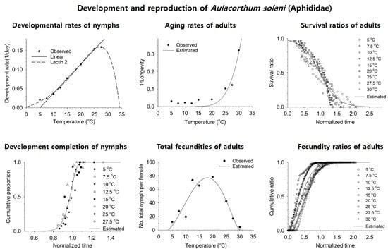
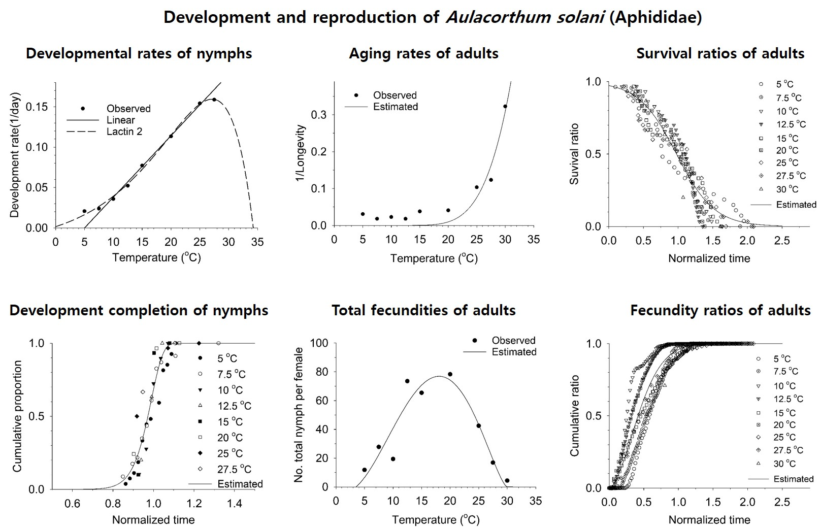
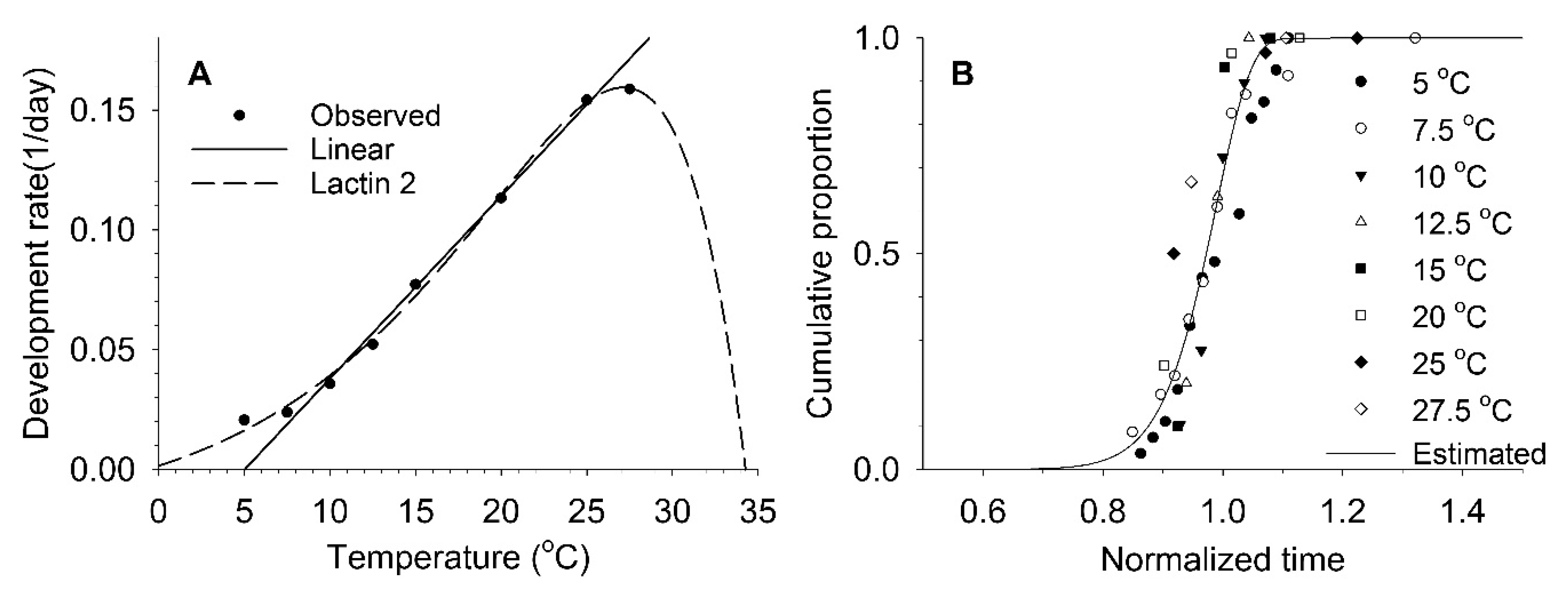
3.2. Estimation of Developmental and Reproductive Patterns Based on Models
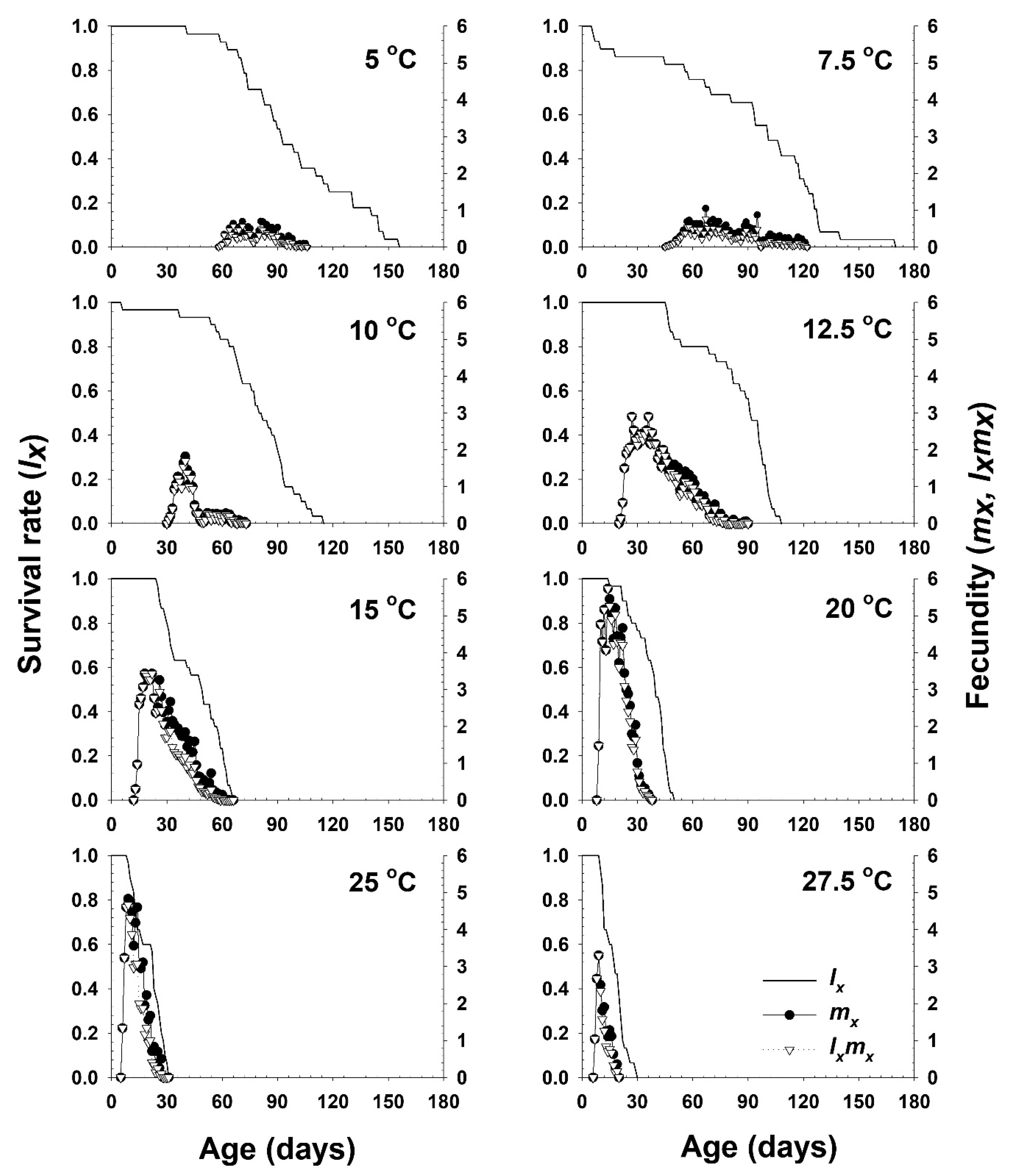
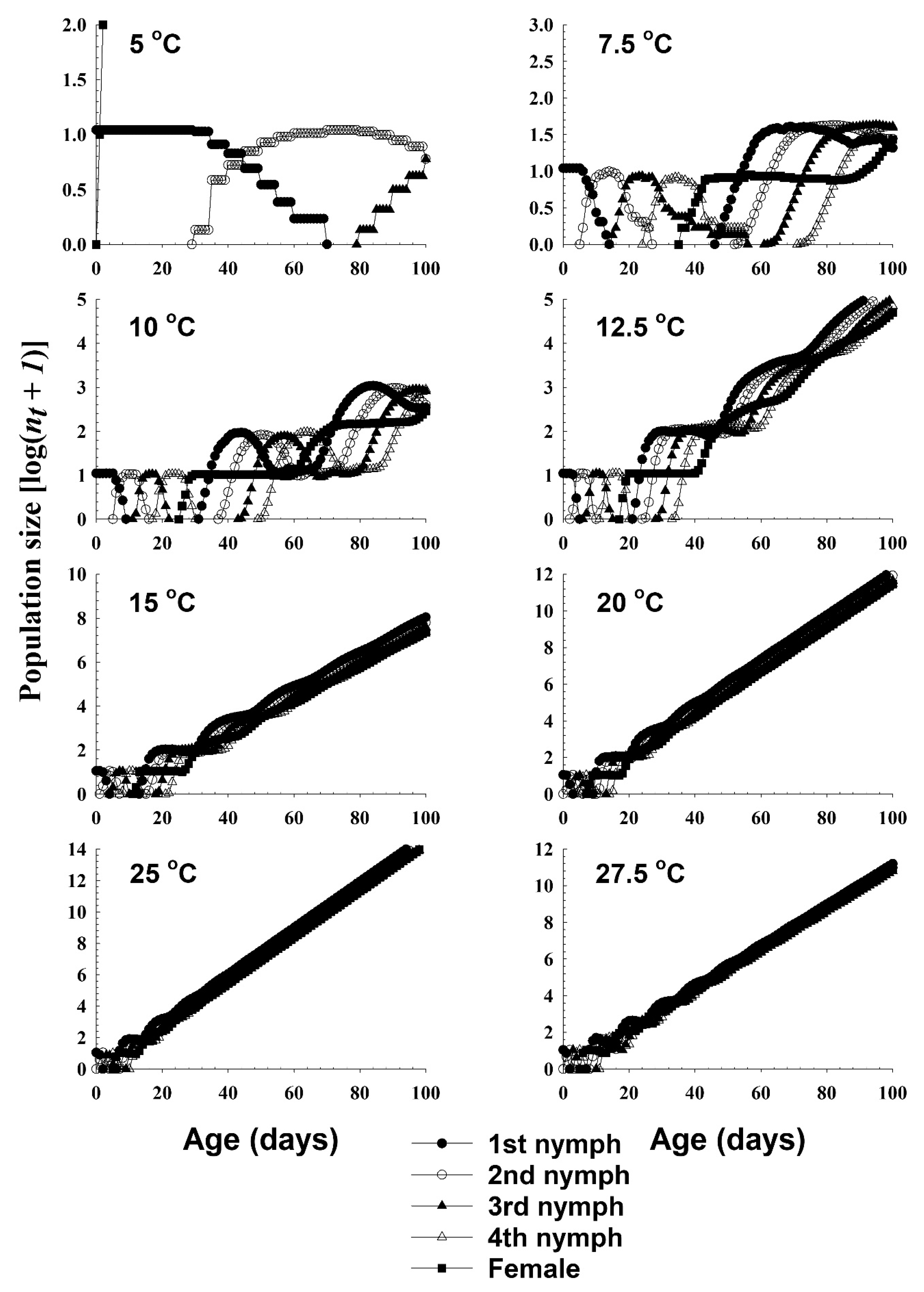
LDT and the degree-days (DD) above LDT required to complete nymphal development (i.e., the thermal constant) were determined to be 5.02 °C and 131.2 DD, respectively, based on the linear development model (Equation (1)) (Table 3 and Figure 1). The LDTs of each separate nymphal instar estimated using the linear model ranged from 5.39 to 6.32 °C (Table 4). The LDT of the nymphal stage overall determined using the Lactin-2 model (Equation (2)) was −1.85 °C (Table 3). The estimated upper lethal temperature (UDT) was 33.9 C. The optimal temperature was estimated to be 26.87 °C. The two development rate models had very high adjusted coefficients of determination (radj2) values, which were ≥0.99 for both models. The data for inter-individual variation in developmental completion were fit well by the model tested (Equation (3)), with a high radj2 value of 0.90 (Table 3 and Figure 1). The model parameters and values derived from this model for each nymphal instar are provided in Table 4.
Aging rate increased exponentially with increasing temperature, and its generalized model (Equation (4)) achieved a high radj2 value of 0.88 (Table 5 and Figure 2). However, the model underestimated observed aging rates between 5 and 20 °C. The total fecundity model (Equation (5)) achieved an radj2 value of 0.74, and estimated that the maximum fecundity of this species on soybean is ca. 76.9 nymphs per adult at an optimum temperature of 18.1 °C. Survival (Equation (6)) and cumulative fecundity (Equation (3)) models applied to the normalized ages of adults fit the observed values well, with high radj2 values.
The age-dependent daily mortality of adults at particular temperatures rapidly decreased with increasing temperature. The age-specific survival rate and fecundity of A. solani are presented in Figure 3. The age-specific survival rate (lx) is the sum of sxj at each age x and is the simplified version of sxj. The curves sharply dropped at an earlier age from 15 °C to 27.5 °C. The daily fecundity at temperatures from 10 to 27.5 °C sharply increased at earlier ages, and slowly decreased thereafter until the final parthenogenesis occurred, while at lower temperatures of 5 and 7.5 °C, daily fecundity values were relatively stable across ages. The highest age-specific fecundities were 0.70 (81 d), 1.04 (67 d), 1.82 (40 d), 2.90 (36 d), 3.43 (22 d), 5.73 (14 d), 4.82 (9 d), and 3.30 (9 d) offspring at 5, 7.5, 10, 12.5, 15, 20, 25, and 27.5 °C, respectively. The peaks of mx and lxmx tended to increase with increasing temperature from 5 °C to 20 °C. The model (Equation (7)) used to generalize the relationship between adult age and daily fecundity fit the observed data well at temperatures between 12.5 and 25 °C, with a high radj2 value over 0.9. The performance of this model at lower (5~10 °C) and higher temperatures (27.5 and 30 °C) than those in this range, however, was relatively poor (Table 6). The model estimated the highest fecundity to be ca. 88.5 nymphs per adult at 20 °C. However, the estimated pre-reproductive periods (p2) in the model were shorter than the observed periods at all temperatures. Although the p2 parameter of the model at 25 °C gave a negative value, it was close to zero. The maximum daily fecundity was estimated to be ca. 6.1 nymphs per adult for a 5.2 day old of adult at 21.3 °C in the age- and temperature-dependent daily fecundity model (Equation (8)) (Table 7).

3.3. Life Table

The intrinsic rate of increase (rm) and the finite rate of increase (λ) from both analyses were highest at 25 °C (0.3349, 0.3377, and 1.40, respectively). Doubling time (DT) was shortest at 25 °C (2.07 and 2.05 days). Net reproductive rate (R0) was highest at 20 °C (77.49 and 78.34 nymphs), and the temperature with the second-highest R0 value was 12.5 °C (73.19 and 73.56 nymphs) (Table 8 and Table 9). The generation time (G) decreased with increasing temperature.
The population growth and stage structure at different temperatures based on the age–stage, two-sex life table is presented in Figure 4. The populations from 20 °C and 25 °C increased significantly faster than those at lower temperature conditions.

4. Discussion

The development of insects can be affected by the nutritional value of their host plant, as well as by temperature. The duration of the nymphal period of A. solani on different host plants, including eggplant (Solanum melongena L. (Solanales: Solanaceae)), fennel (Foeniculum vulgare Mill (Apiales: Apiaceae)), lettuce, pea (Pisum sativum L. (Fabales: Fabaceae)), pansy, potato (Solanum tuberosum L. (Solanales: Solanaceae)), and soybean, are as follows: 48.7–63.15 days at 5 °C, 16.7–28.0 days at 10 °C, 16.9–19.2 days at 12.5 °C, 10.3–13.4 days at 15 °C, 7.2–8.9 days at 20 °C, 6.5–7.4 days at 25 °C, 6.3 days at 27.5 °C (data from this study and Jandricic et al. [20]). The nymphal period of A. solani on the same plant species, soybean, as that used in our study was previously observed to be ca. 20 days at 10 °C by Kim et al. [2], which differed considerably from our result (28 days) at this temperature; however, the results of our study and theirs at other common temperatures were not so different (Table 1). The difference of development time at 10 °C may have been due to the use of different cultivars (Taegwangkong and Paldalkong) in the two studies.
The lowest experimental temperature tested in this study was 2.5 °C, which caused 100% mortality of A. solani nymphs on soybean (Table 1). Similarly, Pozarowska [41] reported no survival of nymphs of this species kept at 2 °C on potato. LDTs estimated for this species with the linear model were 5.02 °C on soybean in this study (Table 3), 4.8 °C on lettuce [19], and 3.69 °C on pansy [20]. LDTs estimated using the linear model are usually different depending on the temperature range used, even within the same experiment, and thus the thermal constants for the completion of development estimated also vary along with these different LDTs. Other estimated LDTs on lettuce were 1.09 °C and 0.08 °C [16,17]. Generally, the LDTs for aphid species are lower than those for members of other insect orders. Indeed, based on data published in the literature for 28 cases from 16 species of aphids, the mean ± SD values of LDT and DD for the completion of development estimated from the linear model were 4.1 ± 1.6 °C and 131.4 ± 38.3 DD, respectively [10]. These values cover all of the LDTs and DDs estimated for the nymphal stages of A. solani in this study (Table 1 and Table 4). The Lactin-2 model estimated the LDT to be −1.85 °C in this study (Table 3), but this value is probably not realistic because we observed that all nymphs died at the much higher temperature of 2.5 °C. The LDT of this species on pansy was previously estimated with the Lactin-2 model to be 4.0 °C [20], which is more realistic. The low LDTs estimated for A. solani indicate that this aphid is adapted to lower temperatures, and as a result of this, its survival rates during the winter in temperate regions should be relatively high. Indeed, the survival of anholocyclic forms of A. solani on weeds over the winter season in Scotland was previously reported [9].
Generally, the development of insects is retarded at temperatures above their optimal temperature. In this study, the nymphal period was not retarded by increasing temperature between 5 and 27.5 °C, and survival was high at all these temperatures. However, the developmental periods of the first, second, and third nymphal instars at 30 °C were longer than those at 27.5 °C. The duration of the fourth instar at 27.5 °C was also longer than that at 25 °C, although this difference was not statistically significant (Table 1). This property was also observed in other studies of A. solani, in which longer nymphal periods occurred at 25 °C than 22.5 °C on lettuce [17], at 28 °C than 25 °C on lettuce [16], and at 30 °C than 25 °C on pansy [20].
At the highest temperature tested in this study, 30 °C, mortality during the nymphal period was 100%, which agreed with the results of two previous studies also conducted on soybean [2,42]. Data for nymphs raised on other host plants are also similar, as 100% mortality was reported to occur at 31 °C on lettuce [16] and high mortality, ca. 88%, at 30 °C and 100% mortality at 35 °C was reported on pansy [20]. However, a study on lettuce produced a different result, in that ca. 97% mortality occurred at 27.5 °C [17]. The Lactin-2 model estimated the value of this species’ upper developmental threshold to be 33.9 °C, which was higher than the range of temperatures observed in this study (Table 1 and Table 3). For nymphs reared on pansy, this parameter was estimated to be 37.6 °C based on the Lactin-2 model, and this value was also higher than the observed temperatures at which high or total mortality occurred [20].
The optimal temperature estimated using the Lactin-2 model for the nymphal development of A. solani on soybean was 26.87 °C in this study, while the optimal temperature for nymphs reared on pansy was previously estimated to be 25.7 °C based on the Lactin-2 model [20].
The range of temperatures (12.5–20 °C) over which we found higher fecundities was similar to that found in other studies, which was 16–22 °C and 12.5–20 °C on lettuce, and 10–20 °C on pansy [15,17,20]. The maximum total fecundities of A. solani estimated were commonly below 90 nymphs per adult in all previous studies, which agrees with our results. However, it appears that high temperatures above 20 °C can suppress the reproduction of A. solani, since we observed that the total fecundity and net reproductive rate (R0) decreased significantly at 25 °C compared to at 20 °C, at which the highest fecundity and R0 values were found (Table 2 and Table 6). Similar results were found in other studies, wherein total fecundity and R0 on lettuce were ca. 68 and 63 nymphs per adult, respectively, at 22 °C, but ca. 18 and 23 nymphs at 25 °C [15]; on pansy, these were ca. 68 and ca. 64 nymphs at 20 °C, but ca. 39 and ca. 37 nymphs at 25 °C [20]. However, these findings should be further confirmed, because Kim et al. [2]’s study rearing this species on soybean showed that the highest fecundity, ca. 83 nymphs per adult, occurred at 25 °C.
Several characteristics of the adult biology of A. solani on soybean in the study described in Kim et al. [2] were quite different from the results of this study. Adult longevities and reproductive periods at 25 °C and 30 °C were much longer in Kim et al. [2] than those in this study. Total fecundities at 10 and 30 °C were also much higher in the previous study [2]. Fecundity is an ideal biological trait for demonstrating the quality of a particular host by measuring the reproductive success of the species. It may be inferred that the differences were caused by the use of different soybean cultivars, and aphid incubation methods, experimental conditions, and differences in the local populations of the aphid in the two studies. Montllor et al. [43] found that when Acythosiphon pisum had been heat-stressed for a period of about 4 h at 39 °C as young (1 day) or as older (5 day) nymphs, A. pisum without pea aphid secondary symbiont (PASS) or pea aphid rickettsia (PAR) failed to reproduce, though not necessarily to survive. Although we did not identify the facultative bacterial secondary symbionts of A. solani in this study, it may be speculated there is a relationship between development and the facultative symbionts of A. solani, because the species could not develop the adult stage at 30 °C and 35 °C but they reproduced at the same temperature.
Life table parameters (the intrinsic rate of increase, finite rate of increase, and net reproductive rate) are appropriate indicators for evaluating the effect of host plants on the development, survival, and fecundity of different populations. The intrinsic rate of increase of this study was higher than that of De Conti et al. [15], but lower than that of Jandricic et al. [20]. The values under lower temperatures (12.5 and 15 °C) in this study were lower and the values at 20 and 25 °C were higher than those of Lee et al. [18]. The aphids may be impaired reproduction and produce few nymphs when fed on different host plant leaves containing low or high levels of soluble nitrogen [44,45,46]. This study presented the advantages of using the age–stage, two-sex life table theory in describing demography. We used survival rate and fecundity data to project the population growth of A. solani to show the advantage of using the age–stage, two-sex life table in revealing the stage structure of insect populations.

5. Conclusions

We investigated several characteristics of the development and reproduction of A. solani on soybean at 10 different temperatures, and described the relationship between temperature and this species’ biology. Our results indicated that A. solani can survive and reproduce on soybean over a temperature range from 5 to 27.5 °C. High rates of reproduction occurred from 12.5 to 20 °C. The estimated LDT, UDT, and Topt for the nymphal development of this species were ca. 5.02 °C, 33.7 °C, and 26.9 °C, respectively. The estimated total fecundity was ca. 76.9 nymphs per adult at 18.1 °C. Most models and their parameters used in this study fitted the observed data well. These models and the life table statistics derived herein should, however, be evaluated under conditions of fluctuating temperatures in the field or in field-simulating conditions before they are applied in future population dynamics studies.

Author Contributions

Conceptualization, J.K.J. and B.Y.S.; Methodology, J.K.J.; Validation, J.J.A. and Y.K.; Formal Analysis, J.K.J.; Investigation, B.Y.S. and E.Y.K.; Resources, S.K.; Writing—Original Draft Preparation, B.Y.S.; Writing—Review & Editing, J.K.J. and J.J.A.; Visualization, J.K.J. and J.J.A.; Project Administration, J.K.J.; Funding Acquisition, J.K.J. All authors have read and agreed to the published version of the manuscript.

Funding

This research was funded by “Cooperative Research Program for Agriculture Science & Technology Development (Project No. PJ01311602)”, Rural Development Administration, Republic of Korea.

Acknowledgments

We are thankful I Hyeon Kim and Soon Il Bae for rearing plants and insects.

Conflicts of Interest

The authors declare no conflict of interest.

References

  1. Holman, J. Host Plant Catalog of Aphids: Palaearctic Region; Springer: New York, NY, USA, 2009; pp. 175–185. [Google Scholar]
  2. Kim, D.-H.; Lee, G.-H.; Park, J.-W.; Hwang, C.-Y. Occurrence aspects and ecological characteristics of foxglove aphid, Aulacorthum solani, Kaltenbach (Homoptera: Aphididae) in soybean. Res. Rept. RDA 1991, 33, 28–32. [Google Scholar]
  3. Lee, J.S.; Yoo, M.; Jung, J.K.; Bilyeu, K.D.; Lee, J.-D. Detection of novel QTLs for foxglove aphid resistance in soybean. Theor. Appl. Genet. 2015, 128, 1481–1488. [Google Scholar] [CrossRef] [PubMed]
  4. Takada, H.; Ono, T.; Torikura, H.; Enokiya, T. Geographic variation in esterase allozymes of Aulacorthum solani (Homoptera: Aphididae) in Japan, in relation to its outbreaks on soybean. Appl. Entomol. Zool. 2006, 41, 595–605. [Google Scholar] [CrossRef] [Green Version]
  5. Hwang, C.Y.; Uhm, K.B.; Choi, K.M. Seasonal occurrence of aphids (Aulacorthum solani K., Aphis glycines M.) and effects of some insecticides on aphids with infurrow treatment in soybean. Korean J. Plant Prot. 1981, 20, 112–116. [Google Scholar]
  6. Leather, S.R. Aspects of aphid overwintering (Homoptera: Aphidinea: Aphididae). Entomol. Gener. 1992, 17, 101–113. [Google Scholar] [CrossRef]
  7. Lee, S.; Holman, J.; Havelka, J. Illustrated Catalogue of Aphididae in the Korean Peninsula. Part I. Subfamily Aphidinae (Hemiptera: Sternorrhyncha); KRIBB & CIS: Chuncheon, Korea, 2002; pp. 106–108. [Google Scholar]
  8. Miyazaki, M. Forms and morphs of aphids. In Aphids Their Biology, Natural Enemies and Control; Minks, A.K., Harrewijn, P., Eds.; Elsevier: New York, NY, USA, 1987; Volume A, pp. 27–50. [Google Scholar]
  9. Turl, L.A.D. The effect of winter weather on the survival of aphid populations on weeds in Scotland. EPPO Bull. 1983, 13, 139–143. [Google Scholar] [CrossRef]
  10. Honěk, A.; Kocourek, F. Temperature and development time in insects: A general relationship between thermal constants. Zool. Jahrbücher Syst. 1990, 117, 401–439. [Google Scholar]
  11. Chown, S.L.; Nicolson, S.W. Insect Physiological Ecology: Mechanisms and Patterns; Oxford University Press: Oxford, UK, 2004; pp. 115–176. [Google Scholar]
  12. Damos, P.; Savopoulou-Soultani, M. Temperature-driven models for insect development and vital thermal requirements. Psyche 2012, 2012, 1–13. [Google Scholar] [CrossRef]
  13. Dixon, A.F.G.; Honěk, A.; Keil, P.; Kotela, M.A.A.; Sizling, A.L.; Jarosik, V. Relationship between the minimum and maximum temperature thresholds for development in insects. Funct. Ecol. 2009, 23, 257–264. [Google Scholar] [CrossRef]
  14. Wagner, T.L.; Wu, H.; Sharpe, P.J.H.; Coulson, R.N. Modeling distribution of insect development time: A literature review and application of Weibull function. Ann. Entomol. Soc. Am. 1984, 77, 475–483. [Google Scholar] [CrossRef]
  15. De Conti, B.F.; Bueno, V.H.P.; Sampaio, M.V.; Sidney, L.A. Reproduction and fertility life table of three aphid species (Macrosiphini) at different temperatures. Rev. Bras. Entomol. 2010, 54, 654–660. [Google Scholar] [CrossRef] [Green Version]
  16. De Conti, B.F.; Bueno, V.H.P.; Sampaio, M.V.; Van Lenteren, J.C. Development and survival of Aulacorthum solani, Macrosiphum euphorbiae and Uroleucon ambrosiae at six temperatures. Bull. Insectol. 2011, 64, 63–68. [Google Scholar]
  17. Lee, S.G.; Kim, H.H.; Kim, T.H.; Park, G.-J.; Kim, K.H.; Kim, J.S. Development model of the foxglove aphid, Aulacorthum solani (Kaltenbach) on lettuce. Korean J. Appl. Entomol. 2008, 47, 359–364. [Google Scholar] [CrossRef]
  18. Lee, S.G.; Kim, H.H.; Kim, T.H.; Park, G.-J.; Kim, K.H.; Kim, J.S. Longevity and life table of the foxglove aphid (Aulacorthum solani K.) adults on lettuce (Lactuca sativa L.). Korean J. Appl. Entomol. 2008, 47, 365–368. [Google Scholar] [CrossRef]
  19. Park, G.-J. Temperature-dependent development and its model of the foxglove aphid, Aulacorthum solani (Kaltenbach) (Homoptera: Aphididae). Master’s Thesis, JeonBuk National University, Jeonju, Korea, 22 August 2008. [Google Scholar]
  20. Jandricic, S.E.; Wraight, S.P.; Bennett, K.C.; Sanderson, J.P. Developmental times and life table statistics of Aulacorthum solani (Hemiptera: Aphididae) at six constant temperatures, with recommendations on the application of temperature-dependent development models. Environ. Entomol. 2010, 39, 1631–1642. [Google Scholar] [CrossRef] [PubMed]
  21. Kingsolver, J.G.; Higgins, J.K.; Augustine, K.E. Fluctuating temperatures and ectotherm growth: Distinguishing non-linear and time-dependent effects. J. Exp. Biol. 2015, 218, 2218–2225. [Google Scholar] [CrossRef] [Green Version]
  22. Chi, H.; Liu, H. Two new methods for the study of insect population ecology. Bull. Inst. Zool. Acad. Sin. 1985, 24, 225–240. [Google Scholar]
  23. Chi, H. Life-table analysis incorporating both sexes and variables development rates among individuals. Environ. Entomol. 1988, 17, 26–34. [Google Scholar] [CrossRef]
  24. SAS Institute Inc. SAS/STAT 9.1 User’s Guide; SAS Institute Inc.: Cary, NC, USA, 2004; pp. 1731–1906. [Google Scholar]
  25. Campbell, A.; Frazer, B.D.; Gilbert, N.; Gutierrrez, A.P.; Markauer, M. Temperature requirements of some aphids and their parasites. J. Appl. Ecol. 1974, 11, 431–438. [Google Scholar] [CrossRef]
  26. Lactin, D.J.; Holliday, N.J.; Johnson, D.I.; Craigen, R. Improved rate model of temperature-dependent development by arthropods. Environ. Entomol. 1995, 24, 68–75. [Google Scholar] [CrossRef]
  27. Weibull, W.A. Statistical distribution function of wide applicability. J. Appl. Mech. 1951, 18, 290–293. [Google Scholar]
  28. Eyring, H. The activated complex in chemical reactions. J. Chem. Phys. 1935, 3, 107–115. [Google Scholar] [CrossRef]
  29. Curry, G.L.; Feldman, R.M. Mathematical Foundations of Population Dynamics; The Texas A&M University Press: College Station, TX, USA, 1987; pp. 31–76. [Google Scholar]
  30. Park, J.H.; Kwon, S.H.; Kim, T.O.; Oh, S.O.; Kim, D.-S. Temperature-dependent development and fecundity of Rhopalosiphum padi (L.) (Hemiptera: Aphididae) on corns. Korean J. Appl. Entomol. 2016, 55, 149–160. [Google Scholar] [CrossRef]
  31. Briere, J.F.; Pracros, P.; LeRoux, A.Y.; Pierre, J.S. A novel rate model of temperature-dependent development for arthropods. Environ. Entomol. 1999, 28, 22–29. [Google Scholar] [CrossRef]
  32. Kim, D.-S.; Lee, J.-H. Oviposition model of Carposina sasakii (Lepidoptera: Carposinidae). Ecol. Model. 2003, 162, 145–153. [Google Scholar] [CrossRef]
  33. Sauvion, N.; Rahbé, Y.; Peumans, W.J.; Van Damme, E.J.M.; Gatehouse, J.A.; Gatehouse, A.M.R. Effects of GNA and other mannose binding lectins on development and fecundity of the peach-potato aphid Myzus persicae. Entomol. Exp. Appl. 1996, 79, 285–293. [Google Scholar] [CrossRef] [Green Version]
  34. Ydergaard, S.; Enkegaard, A.; Brødsgaard, H.F. The predatory mite Hypoaspis miles: Temperature dependent life table characteristics on a diet of sciarid larvae, Bradysia paupera and B. tritici. Entomol. Exp. Appl. 1997, 85, 177–187. [Google Scholar] [CrossRef]
  35. Birch, L.C. The intrinsic rate of natural increase of an insect population. J. Anim. Ecol. 1948, 17, 15–26. [Google Scholar] [CrossRef]
  36. Southwood, T.R.E.; Henderson, P.A. Ecological Methods, 3rd ed.; Blackwell Science Ltd.: Oxford, UK, 2000; pp. 404–436. [Google Scholar]
  37. Chi, H. TWOSEX-MSChart: A Computer Program for the Age-Stage, Two-Sex Life Table Analysis. 2020. Available online: http://140.120.197.173/Ecology/Download/Twosex-MSChart.exe-B100000.rar (accessed on 19 April 2020).
  38. Goodman, D. Optimal life histories, optimal notation, and the value of reproductive value. Am. Nat. 1982, 119, 803–823. [Google Scholar] [CrossRef]
  39. Efron, B.; Tibshirani, R.J. An Introduction to the Bootstrap; Chapman & Hall: New York, NY, USA, 1993; pp. 39–85. [Google Scholar]
  40. Chi, H. TIMING-MSChart: A Computer Program for the Population Projection Based on Age-Stage, Two-Sex Life Table. 2020. Available online: http://140.120.197.173/Ecology/Download/Timing-MSChart.rar (accessed on 19 April 2020).
  41. Pozarowska, B.J. Studies on low temperature survival, reproduction and development in scottish clones of Myzus persicae (Sulzer) and Aulacorthum solani (Kaltenbach) (Hemiptera: Aphididae) susceptible and resistant to organophosphates. Bull. Entomol. Res. 1987, 77, 123–134. [Google Scholar] [CrossRef]
  42. Kikuchi, T.; Katoh, H.; Kagawa, K.; Sonoda, S.; Murai, T. Effects of high temperatures on development and fecundity of Aulacorthum solani (Homoptera: Aphididae) and Aphis glycines (Homoptera: Aphididae). Jpn. J. Appl. Entomol. Zool. 2018, 62, 41–46. [Google Scholar] [CrossRef]
  43. Montllor, C.B.; Maxmen, A.; Purcell, A.H. Facultative bacterial endosymbionts benefit pea aphids Acyrthosiphon pisum under heat stress. Ecol. Entomol. 2002, 27, 189–195. [Google Scholar] [CrossRef]
  44. Awmack, C.S.; Leather, S.R. Host plant quality and fecundity in herbivorous insects. Annu. Rev. Entomol. 2002, 47, 817–844. [Google Scholar] [CrossRef] [PubMed]
  45. Atlihan, R.; Polat-Akkopru, E.; Ozgokce, M.S.; Kasap, I.; Chi, H. Population growth of Dysaphis pyri (Hemiptera: Aphididae) on different pear cultivars with discussion on curve fitting in life table studies. J. Econ. Entomol. 2017, 110, 1890–1898. [Google Scholar] [CrossRef] [PubMed]
  46. Chen, G.-M.; Chi, H.; Wang, R.-C.; Wang, Y.-P.; Xu, Y.-Y.; Li, X.-D.; Yin, P.; Zheng, F.-Q. Demography and uncertainty of population growth of Conogethes punctiferalis (Lepidoptera: Crambidae) reared on five host plants with discussion on some life history statistics. J. Econ. Entomol. 2018, 111, 2143–2152. [Google Scholar] [CrossRef] [PubMed]
Figure 1. Observed values of development rates at constant temperatures and estimated linear (Equation (1)) and nonlinear Lactin-2 model (Equation (2)) curves between temperature and development rates (A), and Weibull distribution curve (Equation (3)) for development completion (B) in A. solani nymphs.
Insects 11 00296 g001
Figure 2. Observed values of the aging rate (A), total fecundity (B), cumulative survival ratio (C), and cumulative fecundity ratio (D), and curves estimated from their generalized models (Equation (4), Equation (5), Equation (6), Equation (3)) in A. solani adults.
Insects 11 00296 g002
Figure 3. The age-specific survival rate (lx), the age-specific fecundity (mx), and the age-specific maternity (lxmx) of A. solani in response to different temperature conditions.
Insects 11 00296 g003
Figure 4. The population growth projection of A. solani in response to different temperature conditions, beginning with an initial population of newly born 10 nymphs.
Insects 11 00296 g004
Table 1. Development duration (days, D) (mean ± SD) and stage-specific mortality (%, M) of Aulacorthum solani nymphs on soybean at constant temperatures.
Temp (°C)First InstarSecond InstarThird InstarFourth InstarTotal Nymph
This StudyThis StudyThis StudyThis StudyThis StudyKim et al. [2] 2
DMDMDMDMDMD2M2
2.516.9 ± 6.2 a 173.325.0 ± 16.5 a 162.5-100.0---100.0
5.09.3 ± 2.3 b3.312.0 ± 1.3 b3.413.4 ± 1.7 a 10.014.3 ± 2.0 a 13.648.7 ± 3.4 a 110.0
7.58.9 ± 2.2 b3.310.7 ± 1.8 b10.312.0 ± 5.5 a3.812.3 ± 1.6 b8.042.4 ± 5.0 b23.3
10.07.2 ± 1.1 c0.06.7 ± 0.6 c3.36.2 ± 0.4 b0.07.9 ± 0.5 c0.028.0 ± 1.1 c3.320.2 ± 4.53.0
12.54.1 ± 0.5 d0.04.6 ± 0.5 cd0.04.6 ± 0.6 bc0.05.8 ± 0.6 d0.019.2 ± 0.7 d0.0
15.03.2 ± 0.6 de0.03.0 ± 0.3 de0.03.1 ± 0.4 bcd0.03.7 ± 0.5 e0.013.0 ± 0.4 e0.013.4 ± 2.63.0
20.02.2 ± 0.5 ef0.02.1 ± 0.3 e0.02.0 ± 0.3 cd0.02.6 ± 0.5 f0.08.9 ± 0.6 f0.07.8 ± 1.20.0
25.01.7 ± 0.5 f0.01.7 ± 0.5 e0.01.4 ± 0.5 d0.01.8 ± 0.4 g0.06.5 ± 0.6 g0.07.0 ± 1.00.0
27.51.6 ± 0.5 f0.01.4 ± 0.5 e0.01.3 ± 0.5 d0.02.0 ± 0.3 fg0.06.3 ± 0.5 g0.0
30.02.0 ± 0.9 ef0.02.1 ± 0.7 e63.35.0 bc90.9-100.0-100.0-100
1 Thirty neonate nymphs were treated at various temperatures. Different letters within a column indicate statistically significant difference among means by Tukey’s HSD test at α = 0.05. ANOVA results were F9,266 = 161.47 (p < 0.0001) for 1st instar nymph, F9,237 = 173.47 (p < 0.0001) for 2nd, F8,224 = 145.79 (p < 0.0001) for 3rd, F7,221 = 707.03 (p < 0.0001) for 4th, and F7,221 = 1,741.79 (p < 0.0001) for total nymphal period. 2 These data are from soybean in Kim et al. [2], where 20 nymphs were replicated and Paldalkong cultivar was used.
Table 2. Developmental duration (days) and fecundity of A. solani adults on soybean at constant temperatures.
Temp (°C)Init. No. 1Longevity (Day)Rep. Rate (%) 3R. No.Pre-Reproductive Period (Day)Reproductive Period (Day)Total Fecundity (No.)Daily Fecundity
This StudyKim et al. [2] 4This StudyThis StudyThis StudyKim et al. [2] 4This StudyKim et al. [2] 4This Study
5.02752.9 ± 30.1 b5 92.62517.4 ± 2.7 a22.4 ± 12.1 b 11.8 ± 5.8 ef 0.6 ± 0.2 d
7.52367.0 ± 25.3 a 82.61912.8 ± 1.4 b45.9 ± 19.4 a 27.8 ± 12.4 d 0.6 ± 0.2 d
10.02953.2 ± 17.8 b52.6 ± 26.7100.0297.1 ± 0.8 c24.5 ± 9.6 b34.8 ± 10.419.4 ± 5.2 de41.8 ± 23.60.9 ± 0.3 d
12.53065.1 ± 20.4 ab 100.0304.6 ± 0.6 d46.0 ± 12.6 a 73.5 ± 12.9 ab 1.7 ± 0.3 c
15.03033.3 ± 14.3 c42.4 ± 21.4100.0302.6 ± 0.5 e28.4 ± 11.9 b28.7 ± 8.365.4 ± 20.9 b58.9 ± 25.72.4 ± 0.4 b
20.03028.9 ± 9.0 c31.4 ± 12.5100.0301.8 ± 0.4 ef21.7 ± 5.9 b26.4 ± 5.278.3 ± 14.6 a78.9 ± 19.43.8 ± 0.6 a
25.03014.2 ± 7.1 d28.2 ± 4.3100.0301.3 ± 0.5 f12.4 ± 6.3 c23.8 ± 3.642.5 ± 18.8 c83.0 ± 21.53.6 ± 0.7 a
27.53011.5 ± 6.0 d 93.3282.5 ± 0.6 e7.3 ± 3.6 cd 16.9 ± 9.3 de 2.3 ± 0.8 b
30.0 2303.7 ± 1.3 d13.3 ± 5.780.0241.5 ± 0.6 f2.6 ± 1.2 d11.2 ± 6.14.4 ± 2.3 f25.4 ± 14.81.7 ± 0.5 c
35.0 4.2 ± 2.1 2.3 ± 1.8 2.5 ± 1.7
1 Initial number means the number of adults that emerged from nymphal stage. 2 The adults at 30 °C were treated separately without examination of their nymphal stages. 3 Reproductive rate was calculated as the percentage of the initial number of adults that produced progeny. 4 These data are from soybean in Kim et al. [2], in which 20 adults were replicated and Paldalkong cultivar was used. 5 Different letters within a column indicate statistically significant difference among means by Tukey’s HSD test at α = 0.05. ANOVA results were F8,250 = 58.09 (p < 0.0001) for longevity, F8,236 = 677.57 (p < 0.0001) for pre-reproductive period, F8,236 = 57.93 (p < 0.0001) for reproductive period, F8,236 = 128.48 (p < 0.0001) for total fecundity, and F8,236 = 158.57 (p < 0.0001) for daily fecundity during reproductive period.
Table 3. Parameters and values derived from the development rate models and the distribution model for A. solani nymphs in Figure 1.
ModelParameters and Derived Estimatesradj2
Developmental rate Linear (Equation (1))a = 0.00762 ± 0.00026, b = -0.03824 ± 0.00420 (Temperature range 7.5~25 °C), LDT = 5.02, DD = 131.190.99
Lactin-2 (Equation (2))Ρ = 0.14202 ± 0.01970, TL (UDT) = 33.88565 ± 1.61807, ΔT = 7.01425 ± 0.95905, λ = −0.01491 ± 0.01322, LDT = −1.85, Topt = 26.870.99
Weibull distribution (Equation (3))η = 0.99247 ± 0.00444, β = 17.94321 ± 1.878290.90
ANOVA results were F1,4 = 857.0 (p < 0.0001) for the linear model, F3,4 = 448.7 (p < 0.0001) for the Lactin-2 model, and F1,40 = 365.0 (p < 0.0001) for the Weibull distribution model. Abbreviations: LDT, lower development threshold; DD, degree-days; UDT, upper development threshold; radj2, adjusted r square value.
Table 4. Parameters and values derived from the linear and nonlinear temperature-dependent development models in separate instars of A. solani nymphs.
ModelParameters and Derived ValuesFirst InstarSecond InstarThird InstarFourth Instar
Lineara (slope)0.03351 ± 0.000930.03579 ± 0.001510.04072 ± 0.003360.0298 ± 0.00178
b (intercept)−0.18052 ± 0.01608−0.20268 ± 0.02740−0.25756 ± 0.05424−0.1702 ± 0.02871
Temp. range(°C)10.0–25.07.5–27.57.5–25.07.5–25.0
LDT and DD5.39, 29.85.66, 27.96.32, 24.65.70, 33.5
radj.21.000.990.960.98
ANOVAF1,3 = 1308.8
(p < 0.0001)
F1,5 = 565.0
(p < 0.0001)
F1,4 = 146.8
(p = 0.0003)
F1,4 = 281.1
(p < 0.0001)
Lactin-2Ρ0.14597 ± 0.011970.18764 ± 0.020630.23443 ± 0.014550.19659 ± 0.02063
TL (UDT)33.78729 ± 0.6046132.08891 ± 0.5106330.30548 ± 0.1148430.34261 ± 0.60381
ΔT6.75625 ± 0.520665.30357 ± 0.567514.25799 ± 0.260865.06637 ± 0.52048
λ−0.024430 ± 0.034850.02808 ± 0.042830.06220 ± 0.030000.01504 ± 0.03185
LDT−8.36- 1- 1- 1
Topt27.0326.7926.0525.28
radj.20.990.970.980.99
ANOVAF3,6 = 409.1
(p < 0.0001)
F3,6 = 121.3
(p < 0.0001)
F3,5 = 188.2
(p < 0.0001)
F3,4 = 214.2
(p < 0.0001)
Weibull η0.96899 ± 0.016530.94956 ± 0.018670.91102 ± 0.020930.96280 ± 0.00995
distributionβ3.91272 ± 0.385307.50896 ± 1.757865.59675 ± 1.0750410.54906 ± 1.46181
radj.20.890.730.780.90
ANOVAF1,43 = 363.5
(p < 0.0001)
F1,30 = 90.3
(p < 0.0001)
F1,28 = 111.4
(p < 0.0001)
F1,27 = 273.5
(p < 0.0001)
1 The parameters could not be calculated. Abbreviation: Topt, optimal temperature.
Table 5. Several models and their parameters for A. solani adults in Figure 3.
ModelParametersradj2
Aging rate (Equation (4))a = 4.70782 ± 7.95564, b = 183.66418 ± 49.243000.88
Total fecundity (Equation (5))a = 0.0074 ± 0.0182, TL = 3.4950 ± 3.0050, TM = 30.0000 ± 3.7360, m = 0.6756 ± 0.38670.74
Survival ratio (Equation (6))γ = 0.97594 ± 0.00988, δ = −0.27363 ± 0.010340.92
Cumulative fecundity ratio (Equation (3))η = 0.51445 ± 0.00655, β = 1.73794 ± 0.055820.91
ANOVA results were F1,7 = 70.96 (p < 0.0001) for aging rate, F3,5 = 11.17 (p = 0.0177) for total fecundity, F1,174 = 1949.19 (p < 0.0001) for survival ratio, and F1,566 = 5751.26 (p < 0.0001) for cumulative fecundity ratio.
Table 6. Parameters estimated from the daily fecundity model (Equation (7)) of A. solani adults at constant temperatures.
Temp (°C)p1p2p3radj.2
5.018.12654 ± 1.311383.98639 ± 0.684770.05573 ± 0.003820.58
7.531.87245 ± 1.521363.74750 ± 0.606150.04654 ± 0.002210.70
10.022.88171 ± 1.724761.52812 ± 0.331400.12175 ± 0.008710.66
12.583.24260 ± 1.990111.21637 ± 0.204260.08076 ± 0.002010.93
15.083.47867 ± 2.649070.22761 ± 0.241330.10680 ± 0.003740.91
20.088.53896 ± 3.645520.18145 ± 0.179750.17008 ± 0.007500.91
25.057.06038 ± 2.09382−0.04473 ± 0.120020.23537 ± 0.009460.94
27.522.04102 ± 1.873250.30660 ± 0.156500.30116 ± 0.025140.81
30.04.90767 ± 0.853560.00785 ± 0.132750.64841 ± 0.120950.61
ANOVA results were F2,107 = 76.82 (p < 0.0001) for 5 °C, F2,125 = 148.62 (p < 0.0001) for 7.5 °C, F2,85 = 88.41 (p < 0.0001) for 10 °C, F2,86 = 627.95 (p < 0.0001) for 12.5 °C, F2,52 = 263.86 (p < 0.0001) for 15 °C, F2,38 = 208.32 (p < 0.0001) for 20 °C, F2,22 = 197.73 (p < 0.0001) for 25 °C, F2,22 = 56.01 (p < 0.0001) for 27.5 °C, and F2,4 = 8.32 (p = 0.0375) for 30 °C.
Table 7. Parameters estimated from the age- and temperature-dependent daily fecundity model (Equation (8)) of A. solani adults.
Parameter Estimatesradj.2
ε = −3.42273 ± 0.11850, θ = 0.02574 ± 0.00096, κ = −0.00074 ± 0.00003, ρ = −3.15503 ± 0.06940, ν = 0.00574 ± 0.00057, ψ = −0.00012 ± 0.000020.90
ANOVA result is F5,562 = 981.4 (p < 0.0001).
Table 8. Life table parameters of A. solani at different constant temperatures using traditional age-specific life table analysis.
Temp. (°C)rmR0 (No.)G (Day)λDT (Day)
5.00.02979.6176.291.0323.37
7.50.040518.5172.081.0417.12
10.00.069918.7141.911.079.92
12.50.122673.1935.021.135.65
15.00.181364.2122.951.203.82
20.00.277477.4915.681.322.50
25.00.334940.6711.061.402.07
27.50.248914.7910.821.282.79
rm: intrinsic rate of increase, R0: net reproductive rate in numbers, G: generation time in days, λ: finite rate of increase, and DT: doubling time of population in days.
Table 9. Life table parameters of A. solani at different constant temperatures using age–stage, two-sex life table analysis.
Temp. (°C)rmR0 (No.)G (Day)λDT (Day)
5.00.0307 h10.51 e76.36 a1.03 h22.61 a
7.50.0402 g18.17 d71.85 b1.04 g17.32 b
10.00.0689 f17.68 d41.66 c1.07 f10.06 c
12.50.1226 e73.56 ab35.05 d1.13 e5.65 d
15.00.1827 d65.29 b22.86 e1.20 d3.79 e
20.00.2774 b78.34 a15.72 f1.32 b2.50 g
25.00.3377 a42.52 c11.09 g1.40 a2.05 h
27.50.2534 c15.79 d10.87 g1.28 c2.74 f
rm: intrinsic rate of increase, R0: net reproductive rate in numbers, G: generation time in days, λ: finite rate of increase, and DT: doubling time of population in days. Means in the same row followed by different letters are significantly different (p < 0.05), as determined by the paired bootstrap test.

