1. Introduction
Rolling Element Bearings (REBs) are important components in mechanical transmission. Understanding the physics involved in these parts is of primary interest to improve the design and modeling of overall systems. REB power losses are still a topic under investigation, as can be seen in several recent articles [
1,
2,
3,
4,
5]. The different sources of dissipation in a bearing are known and presented in [
6], and the main contributions are:
- -
Sliding at the ball/ring contact surface area, which is generated by a speed difference between the two surfaces. This contribution is highly load-dependent and has been studied extensively [
7,
8,
9,
10].
- -
Hydrodynamic rolling at the ball/ring contact inlet. It was first considered by Tevaarwerk [
11], who considered this force as the result of pressure along the contact. More recent works [
12,
13,
14] studied this force as a result of traction and sliding effects.
- -
Oil film shearing at the cage and rings or ball interface. It is modeled as a journal bearing [
15,
16] and is generally negligible [
15].
- -
Drag and churning losses between the ball and the oil/air mixture. These contributions have been studied at high rotational speeds [
15,
16,
17] and are predominant when the product N∙dm is greater than
[
15]. However, for low to moderate speeds, this contribution is limited.
There are two main approaches to estimate REB power losses. The first one is based on a global approach. The idea is to predict the REB power losses without specific knowledge of each contribution and without precise information on the internal geometry and kinematics. In this field, two global models are generally found: Harris–Palmgren [
18,
19] and SKF [
20] models. Previous studies have shown that experimental recalibration is necessary for accurate prediction [
21,
22,
23]. Therefore, this approach is not considered in the present study.
The second approach is a local one. The idea is to calculate power losses from each contribution. It requires precise information about the bearing’s internal geometry (ball diameter, osculation). In the literature, not all the above-mentioned contributions are estimated by similar relationships (e.g., in [
1,
3,
24]). As far as the influence of hydrodynamic rolling on deep groove ball bearings (DGBB) or angular contact ball bearings (ACBB) is concerned, most of the studies estimate this force in the elastohydrodynamic lubricated (EHL) regime for loaded balls. This consideration makes sense as ball bearing (BB) contacts are known to have high contact pressures. A few studies [
25,
26] also considered the iso-viscous rigid (IVR) and piezo-viscous rigid regime (PVR) to estimate the hydrodynamic rolling force on loaded balls. These studies were performed at a very low
product (
and for limited contact loads. On the other hand, it has been shown by Darul et al. [
6] that unloaded BB in DGBB must also be considered in the IVR regime to accurately predict REB power losses. This study also showed that, for moderate speeds (N∙dm product less than
) and low applied loads (Fr < 5%
), most of the power losses are due to hydrodynamic rolling [
21]. This study was carried out on radially loaded DGBB. The aim of this paper is to investigate if this approach is suitable for ACBB. To this end, an oil-jet lubricated ACBB is studied for moderate speeds and for limited axial and radial loads (equivalent load ≤ 5% of the static capacity).
The first part of the article deals with a static model, which is necessary to access contact information. Subsequently, the different lubrication regimes observed in the contacts are described and compared to the ones which may occur in a DGBB. As contact temperature is very influential on the lubrication regime, the mechanical model is coupled to a thermal one which aims to simulate the bearing thermal behavior. Next, the power loss calculations are presented, and the model is compared to experimental measurements for different operating conditions: speed, oil injection temperature, oil flow rate, and radial and axial load. Finally, a specific load case is analyzed to study load-independent power losses in the ACBB.
2. Static Model
A static model, according to Jones’ analysis [
7] and detailed in [
19], has been implemented to evaluate power dissipation at each contact point within the REB. This section provides a concise summary of the fundamental procedures employed.
2.1. REB Geometry
The macro-geometry (outer and inner diameters, etc.) of the REB is assumed to be known. However, other parameters must be evaluated to compute the static method:
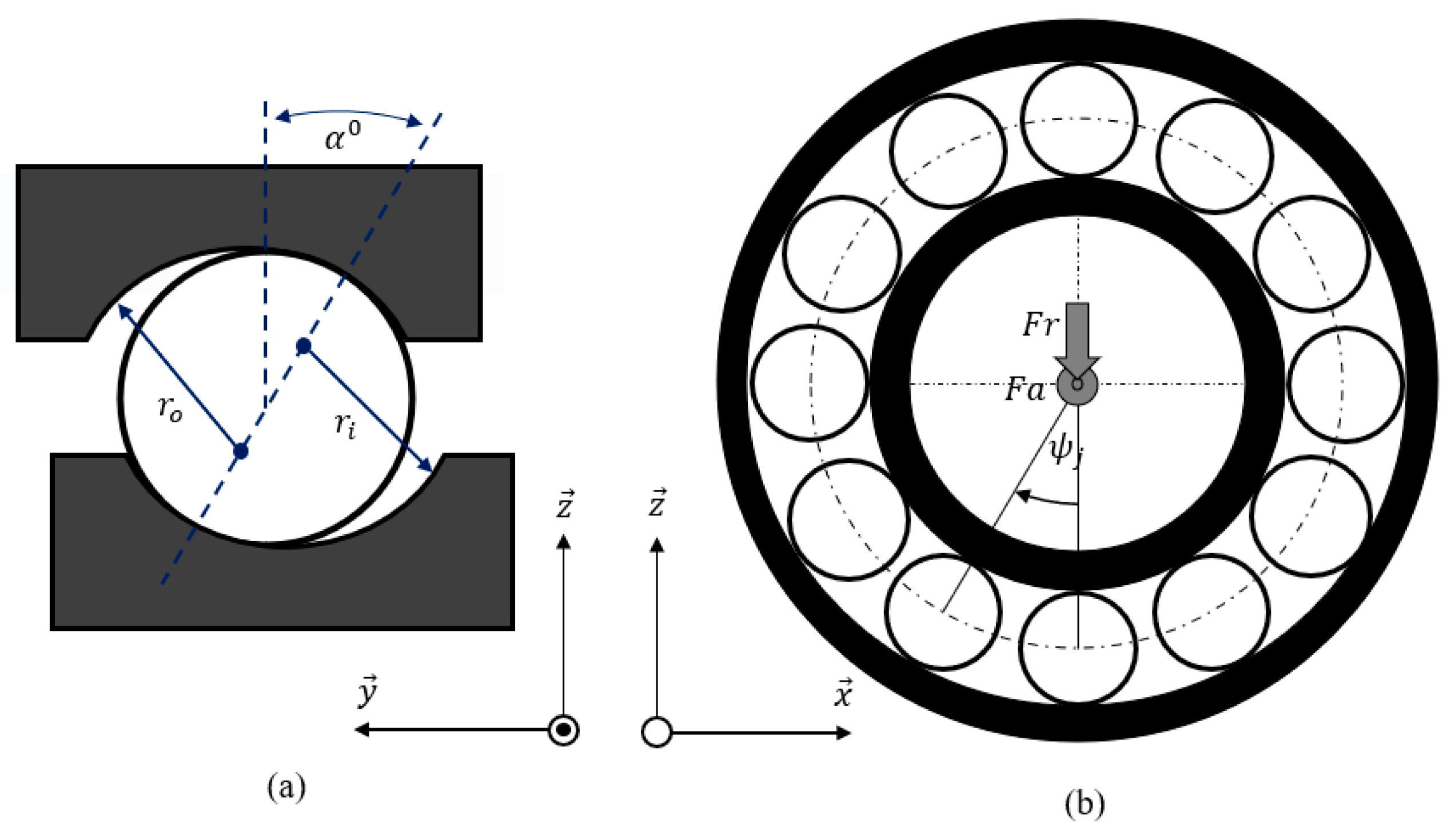
(a) The free contact angle (when no load is applied)
(
Figure 1a) is defined as:
where
is the diametral clearance of the REB and
is the distance between raceway groove curvature centers (
, defined as:
The free contact angle is given by manufacturers for ACBB.
(b) The geometrical ratio
:
where
is the contact angle under loading, depending on
.
is the ball diameter and
is the REB mean diameter.
(c) The equivalent radii in the rolling direction (
) and the transverse one (
are defined for inner and outer rings as:
2.2. Distribution of Internal Loading
The aim is to calculate the load applied to each ball (
Qnj) located at a position
ψj (
Figure 1b). In the present study, the speed range is moderate. Neither centrifugal force nor gyroscopic moment are considered, resulting in similar contact angles and loads on the inner and outer rings. From this hypothesis, the global REB equilibrium can be written as:
and the load
is related to the REB radial displacement
and axial displacement
:
where
is a load-deflection factor defined in [
19].
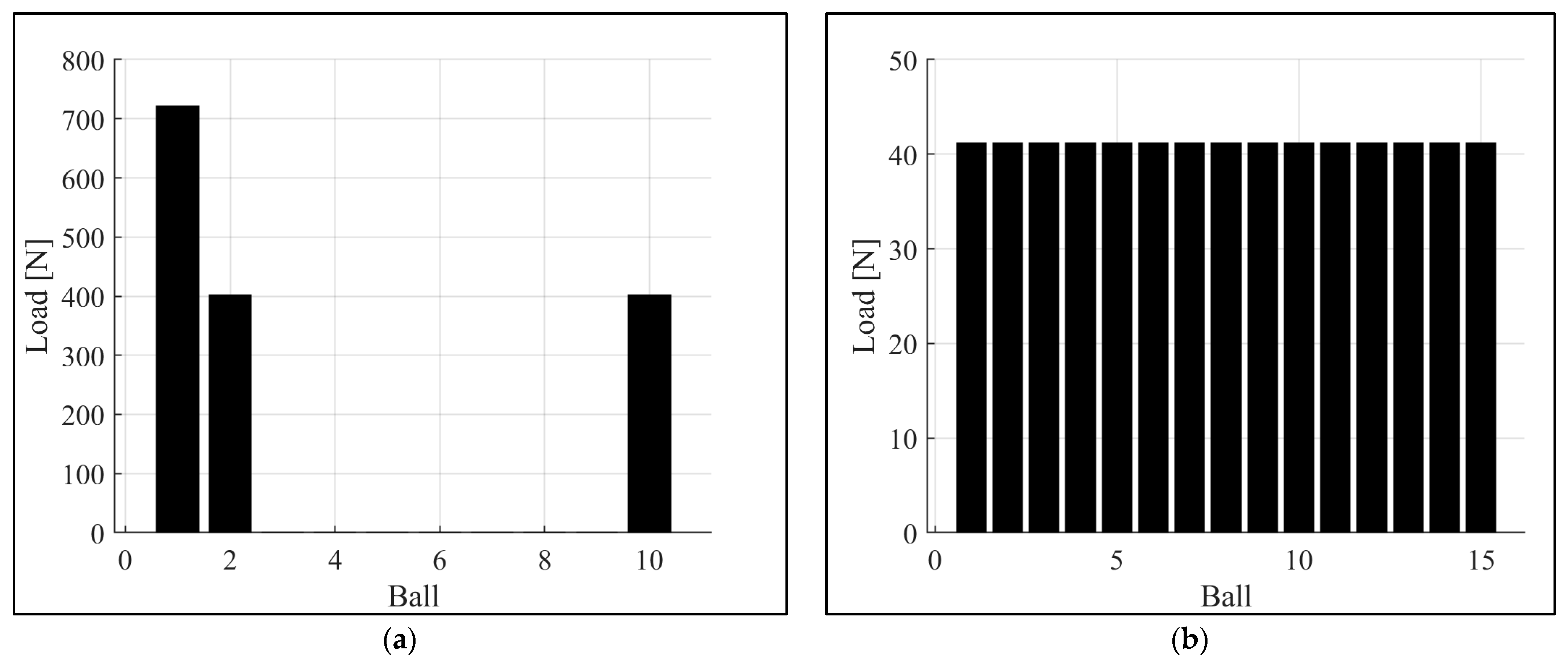
Finally, the global equilibrium is reached for an optimal value
and
. A set of simulations is performed for a DGBB and an ACBB. The bearing and the material properties are given in
Table 1 and
Table 2. A radial load of 1 kN is applied on the DGBB. An axial load of 400 N is applied on the ACBB. The load distribution is shown in
Figure 2. For the radially loaded DGBB, there is a loaded zone and an unloaded one. For the axially loaded ACBB, there is only a loaded zone. It is worth noting that the contact load applied to the loaded balls in the DGBB is much greater than the load applied to each RE in the ACBB. Then, one can wonder if the contact load in the ACBB would be sufficient to reach the EHL regime. This question can be answered by examining the lubrication regime of each ball.
3. Lubrication Regime in Full Film
To investigate the lubrication regime on each contact, Moes’ parameters [
27] are used.
3.1. Moes’ Parameters
Depending on the operating conditions, represented by
L and
N parameters, the dimensionless oil film thickness
H can be estimated:
with
and
U*,
G* or
W* as the Dowson’s parameters [
28]:
The rolling velocity
is calculated as the average point of contact velocity of both the ring and the rolling element:
The ball rotation speed
and the cage rotational speed
are defined in [
19].
3.2. Mapping the Lubrication Regime
It is necessary to reconstruct the Moes’ map since it relies on the ellipticity of the contact. The map is created using the asymptotic solutions of each lubrication regime, as thoroughly explained in [
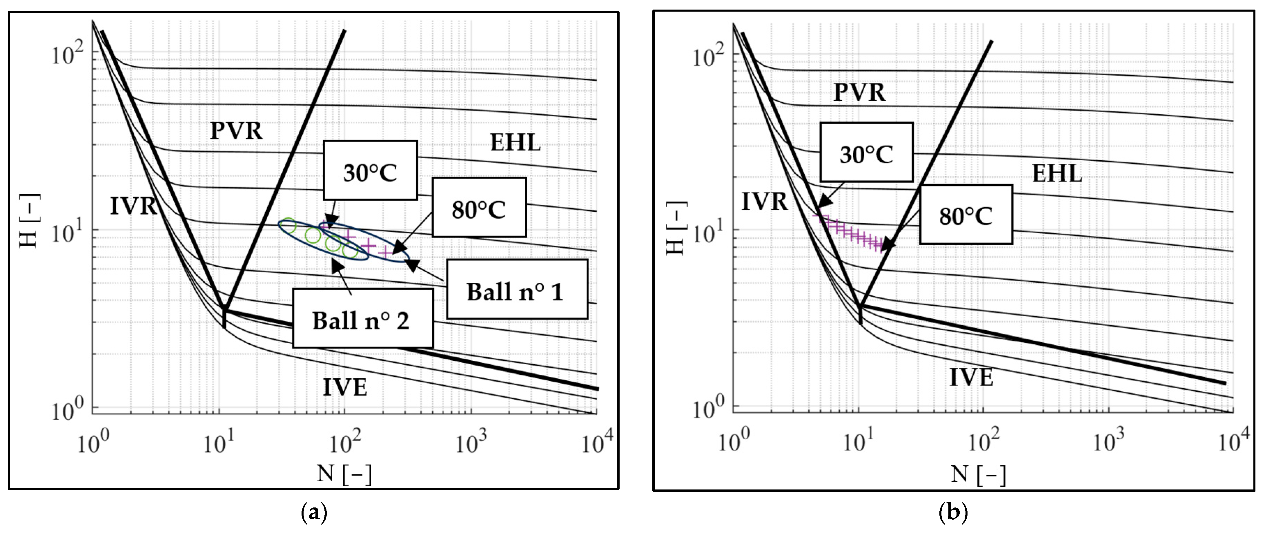
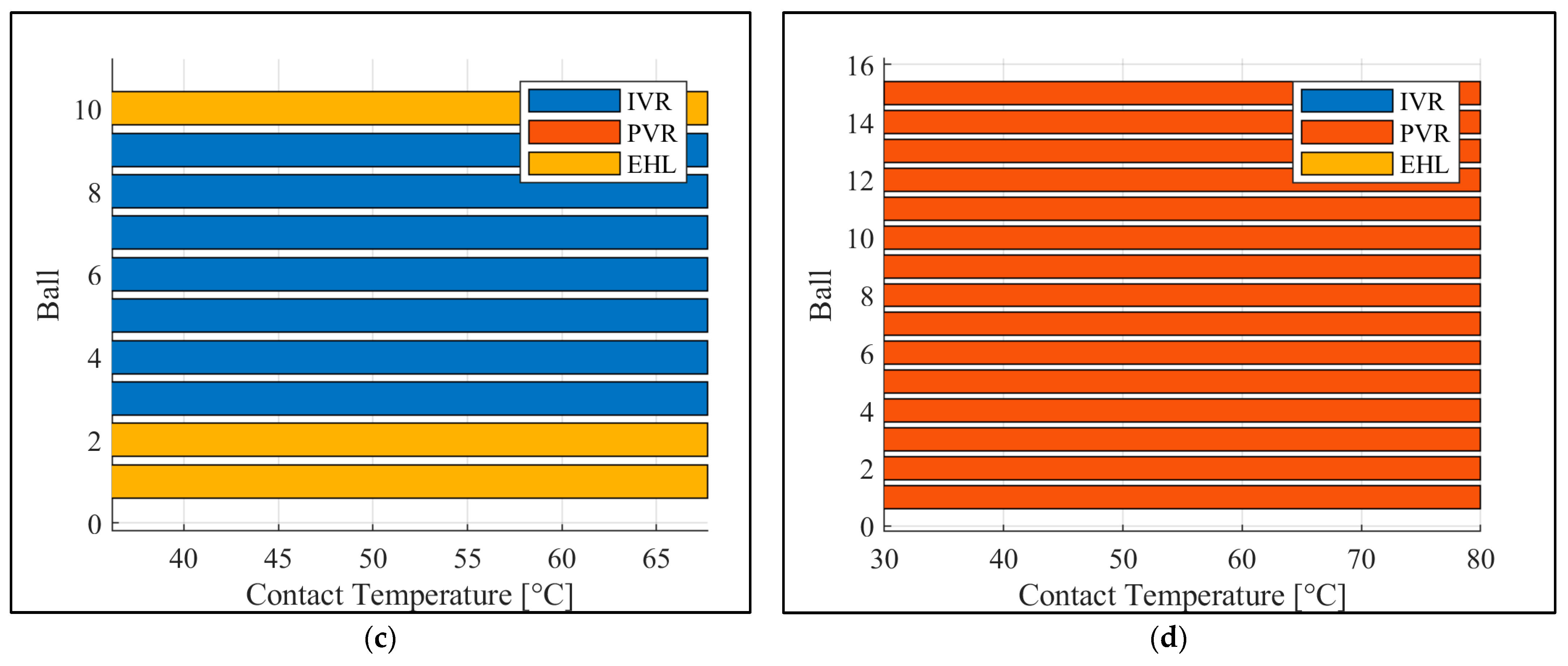
27]. The outcomes of this mapping are illustrated in
Figure 3a, where the different lubrication regimes are also represented. Simulations were run for the above-mentioned DGBB and ACBB, using the loading conditions defined in
Section 2, a rotational speed of 6500 rpm, and a mineral oil with characteristics given in
Table 3. The dimensionless oil film thickness for each ball was plotted for different contact temperatures ranging from 30 °C to 80 °C. For the DGBB (a), it is evident that the lubrication regime for loaded RE is in the EHL zone (as an example, regimes associated with two different loaded balls are plotted in
Figure 3a). For the unloaded balls, the lubrication regime is IVR. However, for the ACBB (b), all RE are loaded and the points are not located in the EHL zone but in the piezo-viscous rigid (PVR) regime. Based on this behavior, two points can be noticed here:
- -
The ball lubrication regime may change from one ball to another, due to the load distribution.
- -
The ball lubrication regime may change according to contact temperature.
Another way to visualize the regime change is proposed by the authors. The idea is to plot the evolution of the lubrication regime for each ball (contact load constant) as a function of the contact temperature. This visualization, shown in
Figure 3c for DGBB and
Figure 3d for ACBB, makes it possible to highlight the influence of contact temperature on the lubrication regime.
A first conclusion can be drawn from this study: the lubrication regime of ACBB RE is not as binary as for radially loaded DGBB. For ACBB, RE are neither in hydrodynamics nor in EHL, but between these two regimes. This must be considered when calculating the power losses.
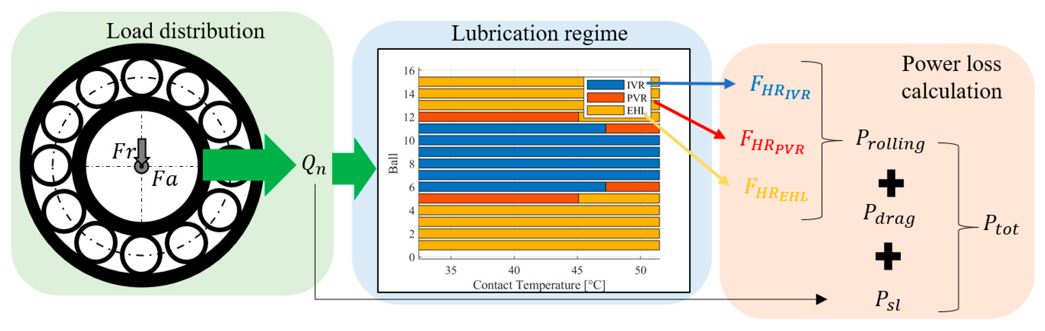
4. Power Loss Modeling
To estimate REB power losses, three contributions are considered: sliding, hydrodynamic rolling, and drag losses. Other contributions, such as elastic rolling resistance or cage interactions, are neglected. Sliding and hydrodynamic rolling occur in the contact area, with an ellipse for BB. The dimensions of this area can be calculated by estimating the load distribution.
4.1. Ball/Ring Contact Area
For a given ball n°j,
is the ellipse dimension in the transverse rolling direction (
):
and
b the ellipse dimension in the rolling direction (
:
with
the equivalent Young’s modulus;
the curvature sum; and
and
the ellipse dimensionless parameters, given in [
19].
Moreover, the maximal Hertz pressure on the contact can be estimated by:
4.2. Sliding
Assuming a constant friction coefficient
, the sliding force on each contact can be estimated from [
29] as:
As a first approximation,
is assumed to be 0.05, consistent with global models found in the literature [
20].
The sliding velocity
can be estimated from Jones [
7] and Harris analyses [
19]. Finally, power losses due to sliding on inner and outer rings are:
4.3. Hydrodynamic Rolling
Hydrodynamic rolling is due to an asymmetric pressure distribution. This is directly linked to the oil film thickness and so to the lubrication regime. As has been shown previously, for low load applications, the lubrication regimes covered are IVR, PVR, and EHL. Hence, the hydrodynamic rolling contribution is not the same for each regime.
- -
For the IVR regime, hydrodynamic rolling can be estimated using Houpert’s work [
30]:
- -
For the EHL regime, the works of Tevaarwerk [
11] or Houpert [
31] can be used:
- -
For PVR regime, Biboulet’s work [
31] can be implemented. It enables a smooth transition from IVR to EHL regimes. This formula has also been used in [
26]:
Finally, power losses from hydrodynamic rolling are calculated by using the rolling velocity defined in Equation (11):
4.4. Drag Losses
It is assumed that the rolling elements are moving through a fluid that is a mixture of air and oil. Then, the estimation of drag losses is achieved using Pouly’s work [
15]:
with
as the mixture density,
as the drag coefficient, and
as the cross-sectional area. These parameters are defined in [
15].
The three contributions considered in this study have been described. These models enable the total REB power loss to be estimated, as shown in
Figure 4. As it has been underlined that the ball lubrication regime may change with contact temperature, this dissipation calculation has to be associated with a thermal model. To this end, a thermal network is used.
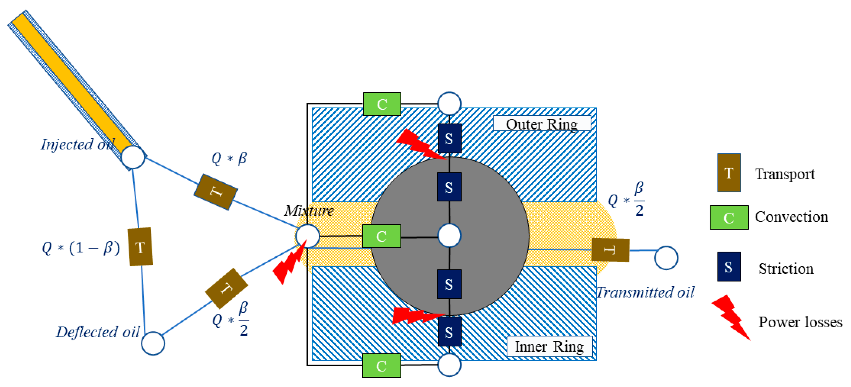
4.5. Thermal Model
The thermal network implemented is based on Pouly’s work [
15] for the bearing modelling and on Brossier’s work [
23] for the oil injection modelling. Concerning the oil flow injection rate
, only a part of the injected oil passes through the bearing. The coefficient of penetration
, which is approximately 0.4 [
23], indicates this. The thermal model, in
Figure 5, requires the bearing inner ring (IR) and the bearing outer ring (OR) measurements. From that, power losses (rolling and sliding) are injected at the IR/RE and OR/RE contacts, and at the air/oil mixture inside the REB (drag losses). Solving the thermal equilibrium results in the temperature of the ball. Therefore, it is assumed that the temperature at the point of contact is the average temperature of the ring and the RE.
5. Experimental Investigation
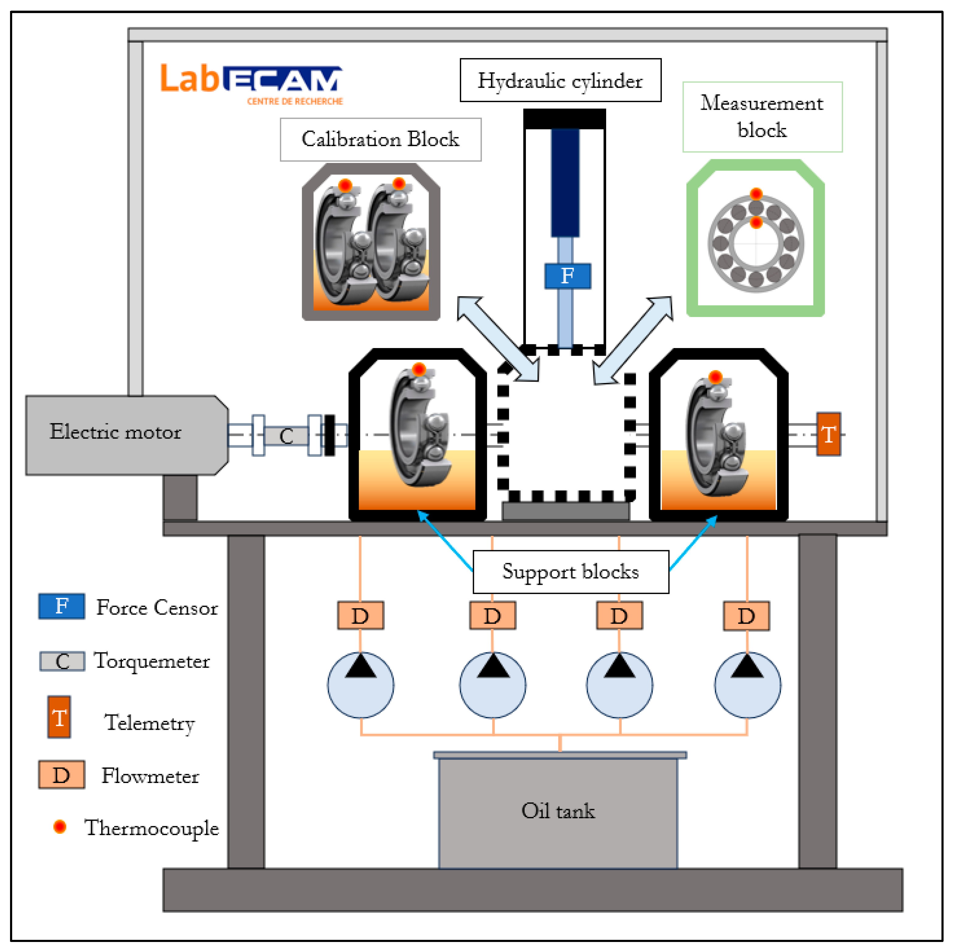
5.1. Test Rig and Test Procedure
The test rig used is presented in [
21,
23]. Only the most relevant details are presented here. The test rig is modular. It is composed of a motor, a torquemeter, two identical oil-bath lubricated “support blocks”, and a “measurement block”. The test rig architecture is presented in
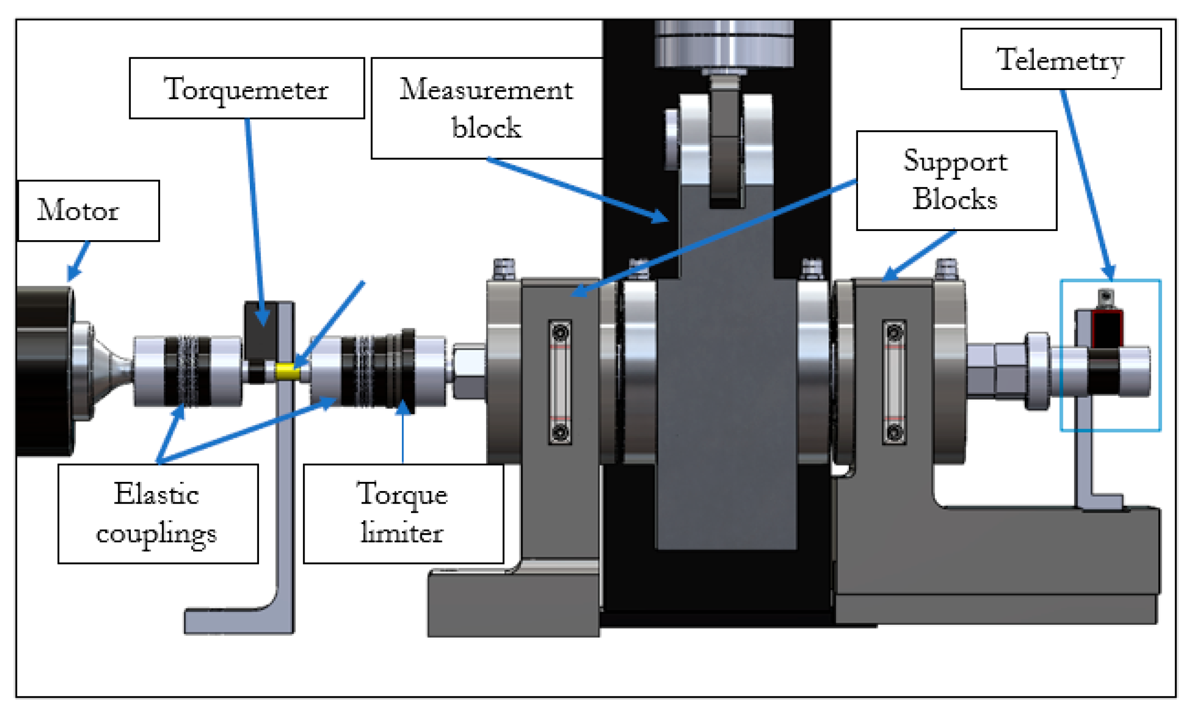
Figure 6 and a visualization is shown in
Figure 7.
5.1.1. Limits and Measurements Performed during This Test Campaign
For this study, the measurement block contains two 7210 REBs (see
Table 1). The tested operating conditions are associated with a maximum rotational speed equal to 8070 rpm, a maximum radial load equal to 1.5 kN, and a maximum axial load equal to 650 N. The OR and IR temperatures are measured with thermocouples (a telemetry device is used for the IR). Other temperatures can be measured, such as for ambient air, block surface, oil injection temperature, etc. The radial load is applied with a hydraulic cylinder. Axial load is applied with corrugated lock washers. Oil is injected using a peristaltic pump. The total shaft torque loss is measured with the torquemeter. The REB torque loss is obtained by subtracting the REB support block torque. A calibration phase is therefore required.
5.1.2. Calibration
This phase is necessary to isolate the power losses of the tested REB from the total measured torque. The objective is to estimate the power dissipation of the support block as a function of speed, loads and outer ring temperatures. As explained in [
21], a calibration block is used instead of the measurement one. This block has two lip seals and two oil-bath lubricated REBs which are identical to the ones used in the support blocks (DGBB). The calibration process takes place in two steps. The first one consists of the measurement of the lip seal power losses. The second one refers to the measure of support REB resistive torque. This procedure is repeated for several speeds, loads, and temperatures. Therefore, the support blocks are characterized, and tests can be performed.
5.1.3. Range and Accuracy
The torquemeter used is a non-contact one. Its full scale is and its accuracy is about . Temperatures are measured with type T thermocouples. Their accuracy is within the range of to . The force sensor has a nominal load of 20 kN and an accuracy of 0.4% of the nominal value. The oil flow accuracy is approximately 5%.
5.2. Rolling Element Bearing and Test Matrix
5.2.1. Oil Lubrication
A mineral oil is used to perform tests. Its physical properties are presented in
Table 2. The oil flow rate is controlled with a peristaltic pump (two oil flow rates were tested: 10 L/h and 15 L/h) and the oil is heated at 50 °C or 70 °C. Oil temperature injection is measured just before injection.
5.2.2. Rotational Speed
The impact of the rotational speed has been tested from 3200 rpm to 8070 rpm. Two intermediate speeds (4800 rpm and 6500 rpm) have been investigated.
5.2.3. Load
As this study aims to focus on limited applied load, the radial load has been changed from 50 N to 1.5 kN ( of the static capacity). Regarding the axial load, a preload is applied to the bearing from 225 N to 675 N.
5.2.4. Test Matrix
Finally, the test matrix is indicated in
Table 4.
5.3. Power Loss Measurement Results
This part investigates the power loss measurement results obtained with the 7210 ACBB. The influence of each parameter is studied.
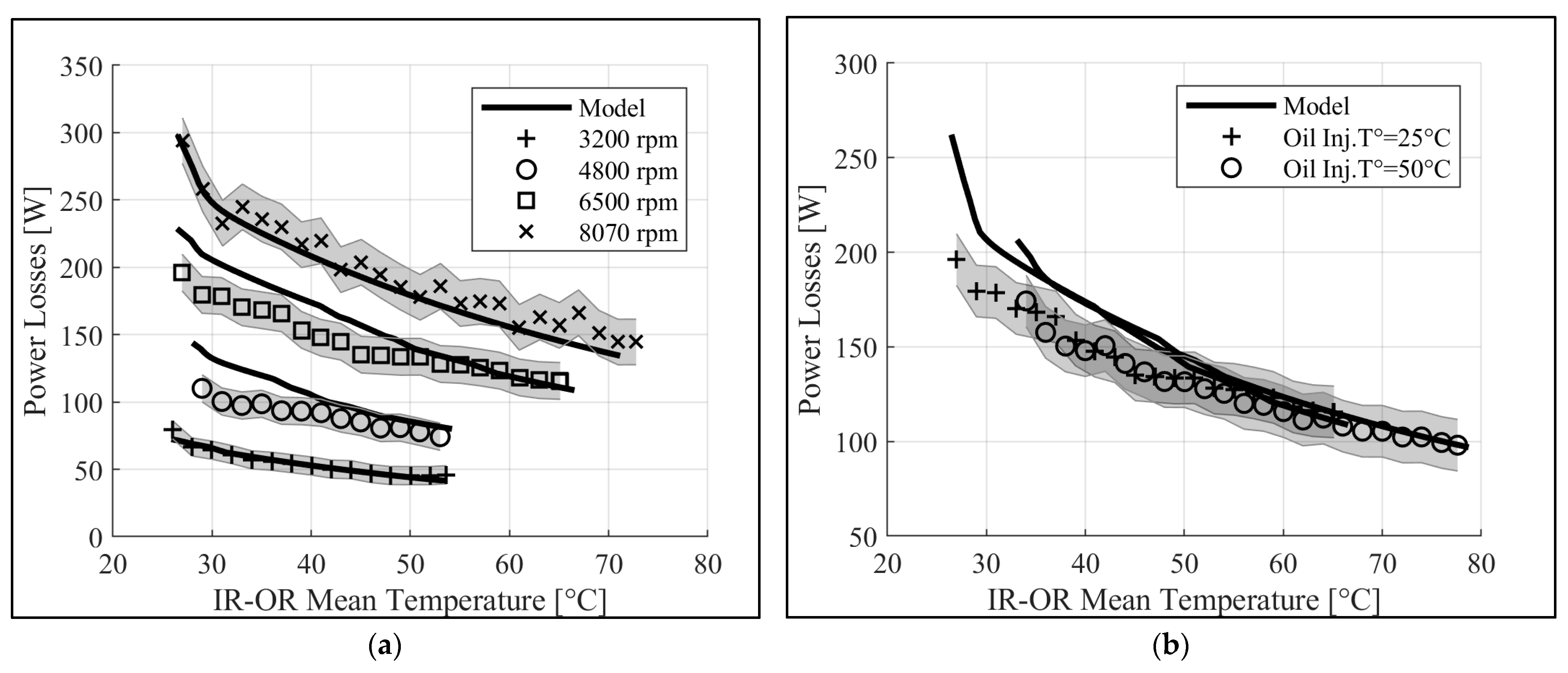
5.3.1. Evolution with Speed
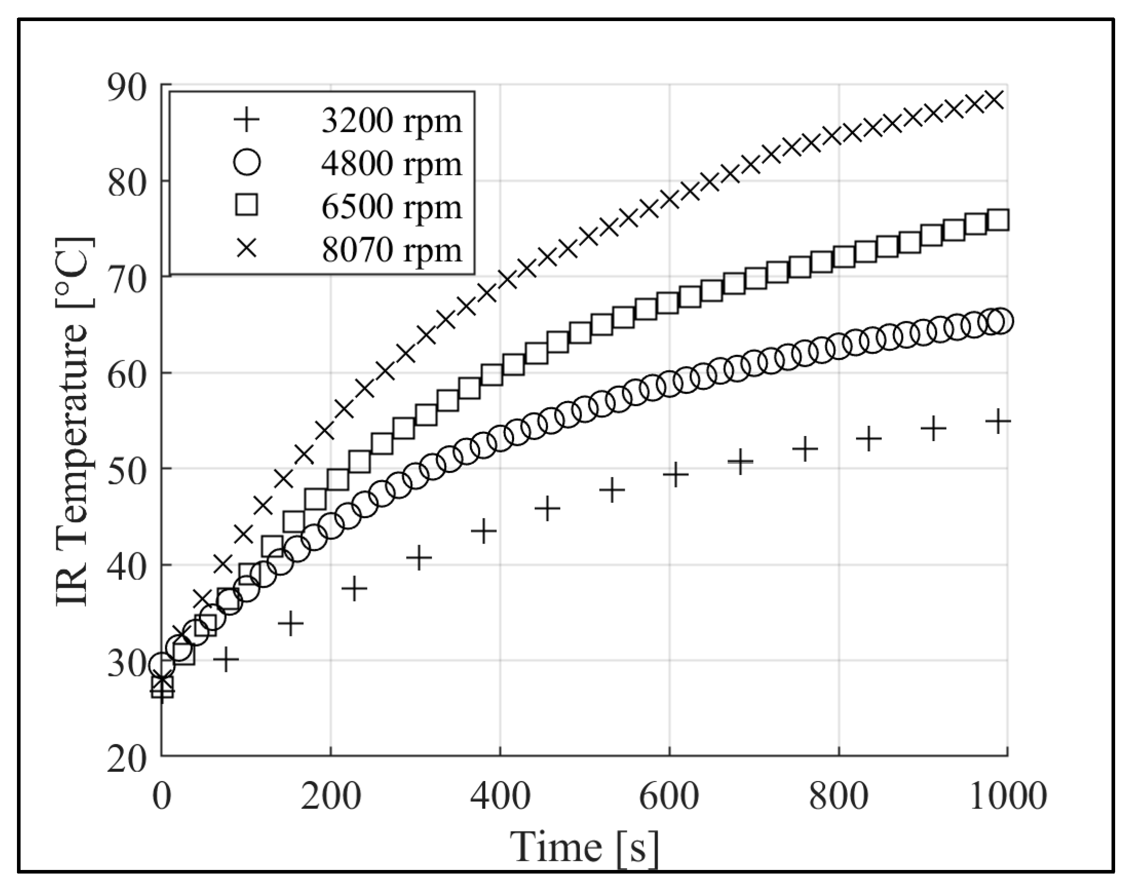
Figure 8 shows the evolution of the inner ring temperature for different speeds. All the other parameters are identical for these experiments referring to test n°1 (
Table 4). It can be observed that the higher the speed is, the faster the IR heats up.
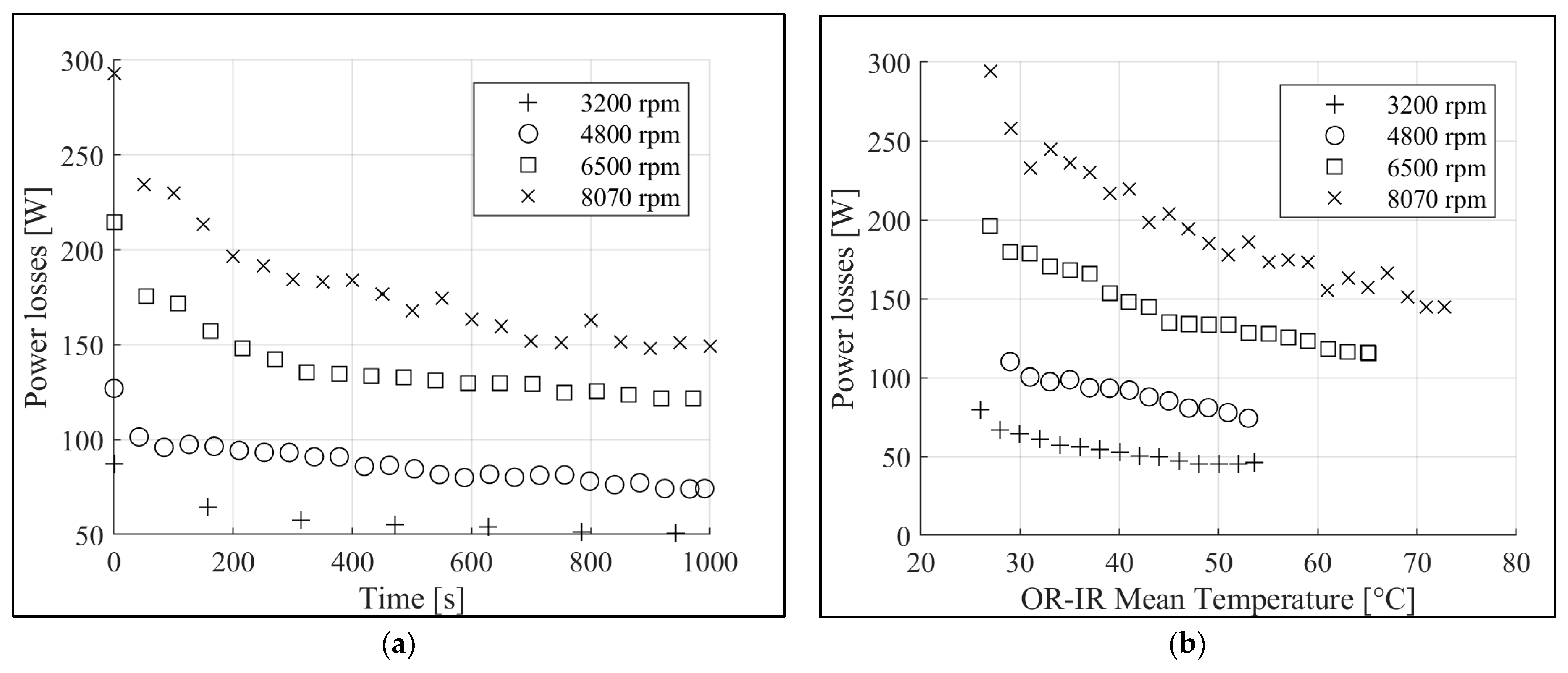
The corresponding power losses are plotted in
Figure 9a. First of all, it can be seen that power losses decrease with time. This behavior can be explained by the oil viscosity decrease as the bearing heats up. Moreover, power losses increase with speed. But, since the REB thermal behavior is not identical for the different curves (for example, at 1000 s, the IR temperature is around 90 °C at 8070 rpm and 55 °C at 3200 rpm), it seems more relevant to compare these evolutions at the same thermal equilibrium. For this reason, in
Figure 9b power losses are plotted with respect to the OR-IR mean temperature. It can be concluded that, at an identical mean temperature, power losses are multiplied by 3 when the speed is twice higher. Furthermore, the OR-IR mean temperature studied here is included in the following range: (25–70 °C).
5.3.2. Evolution with Oil Injection Temperature
Figure 10 shows the evolution of the power losses for two different oil injection temperatures (25 °C and 50 °C) at 6500 rpm (referring to test n°2). This figure highlights that power losses are not modified by the oil injection temperature. As explain by Dowson and Higginson [
28], these findings confirm that the controlling viscosity is associated with the bulk temperature of the REB elements and not with the oil injection one. Therefore, changing the oil temperature can affect the thermal behavior of the bearing, but not the losses directly.
5.3.3. Evolution with Oil Flow Rate
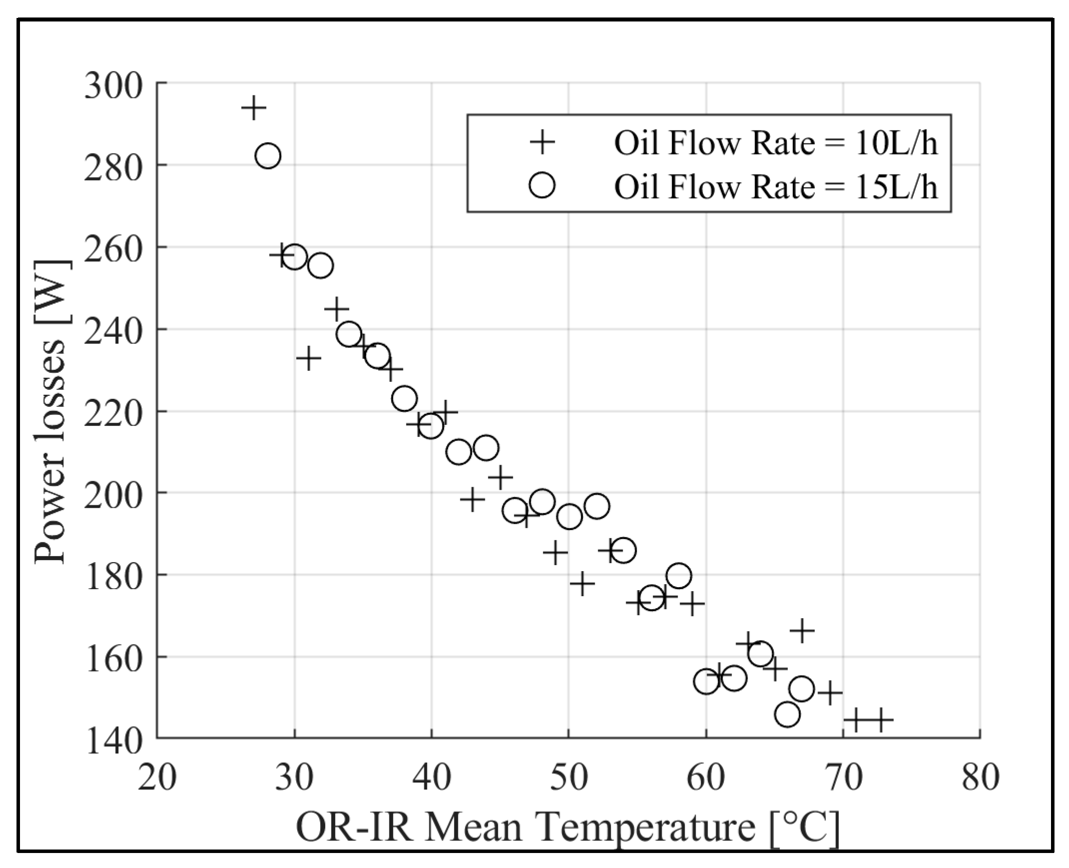
In
Figure 11, the evolution of the power losses is plotted for two different oil flow rates (10 L/h and 15 L/h) at 8070 rpm (referring to test n°3). The power losses are slightly modified by the oil flow rate. This is due to the speed regime, which is moderate in this case study. Indeed, the drag contribution, which is the only one that depends on the oil flow rate, is not predominant at moderate rotational speed.
5.3.4. Evolution with Axial Preload
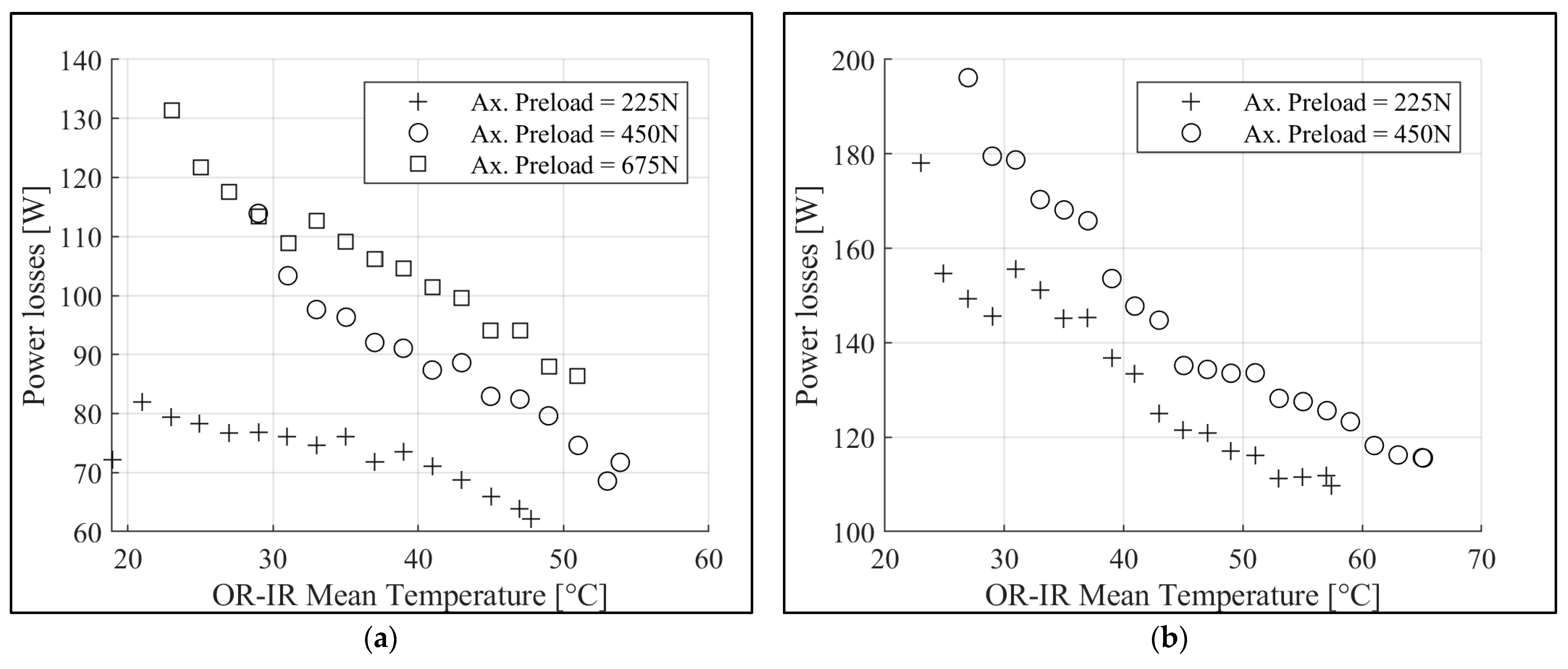
The evolution of power losses for different axial preloads is shown in
Figure 12. In
Figure 12a, the radial load is equal to 0 N, and three axial preloads are tested at 4800 rpm (referring to test n°4). In
Figure 12b, the radial load is equal to 650 N, and two axial preloads are tested at 6500 rpm (referring to test n°5). For all cases, increasing the axial preload increases power losses. These observations, for different operating conditions, are consistent with global power loss models [
18,
19,
20].
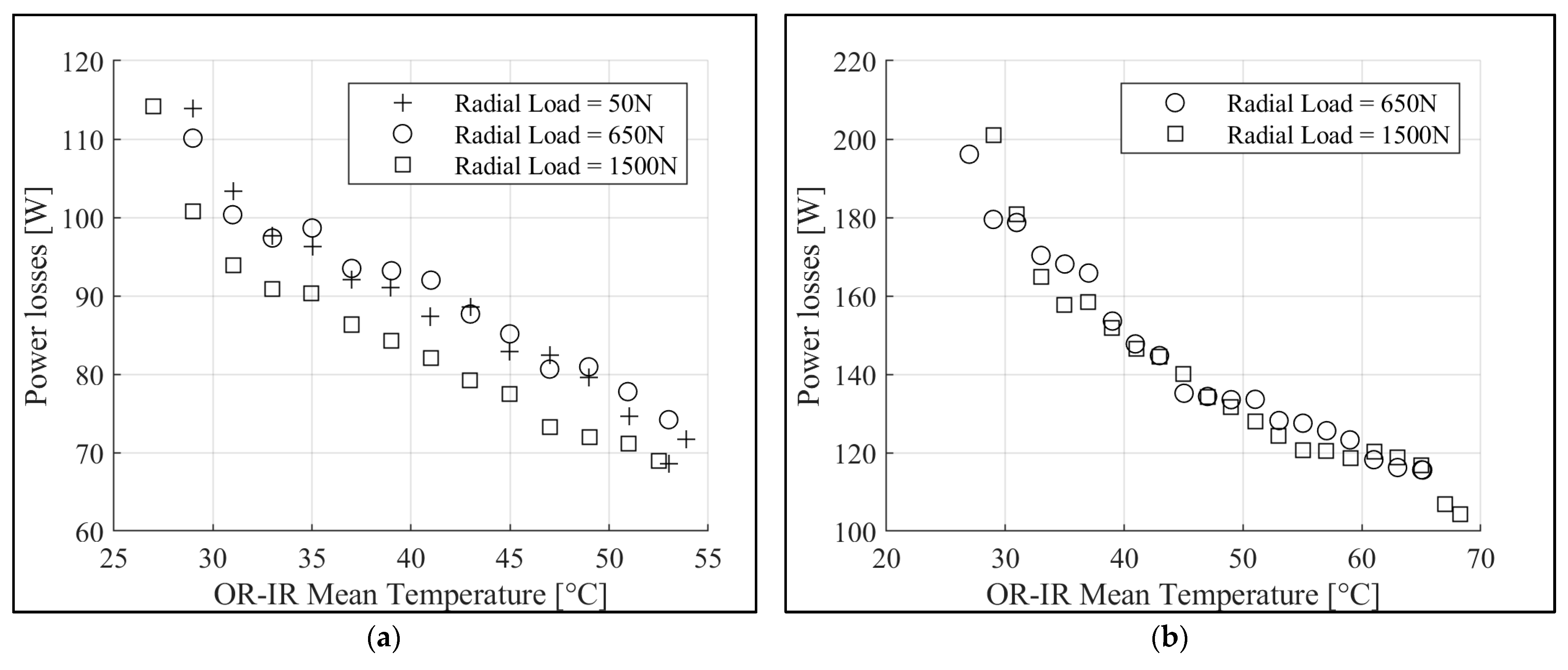
5.3.5. Evolution with Radial Load
The evolution of power losses for different radial loads is shown in
Figure 13. In
Figure 13a, the axial preload is equal to 450 N and three radial loads are tested at 4800 rpm (referring to test n°6). In
Figure 13b, the axial preload is equal to 450 N and two radial loads are tested at 6500 rpm (referring to test n°7). These figures underline that power losses are almost uninfluenced by the radial load. This result is quite surprising and needs further investigation in the next part of the paper through the use of the developed model.
6. Comparison between Measurements and Power Loss Calculations
6.1. Comparison According to Different Parameters
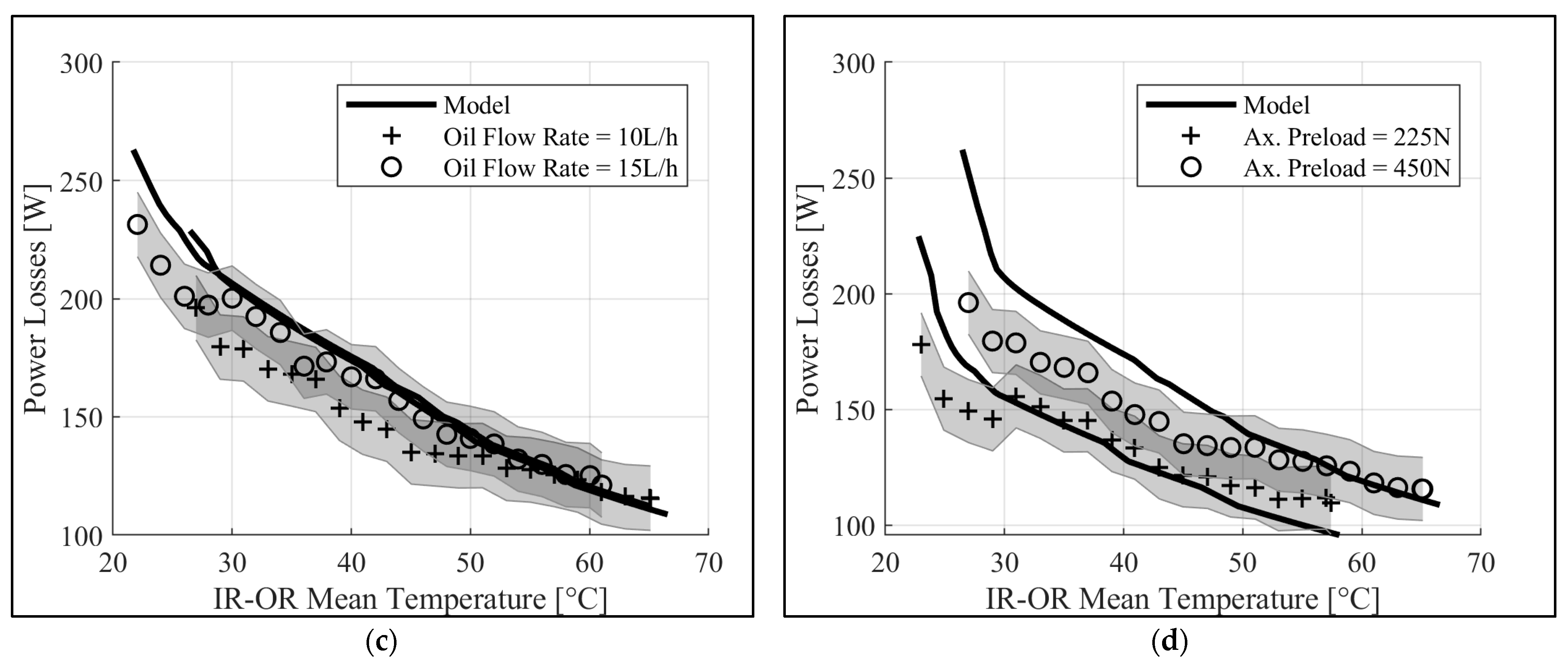
The experiments are compared with the presented model.
Figure 14 shows the comparison for different parameters that have been investigated through the experimental campaign. The black curves represent the power losses calculated with the developed model. The gray shaded areas represent the measurement uncertainty. Several points can be highlighted from these comparisons:
- -
In
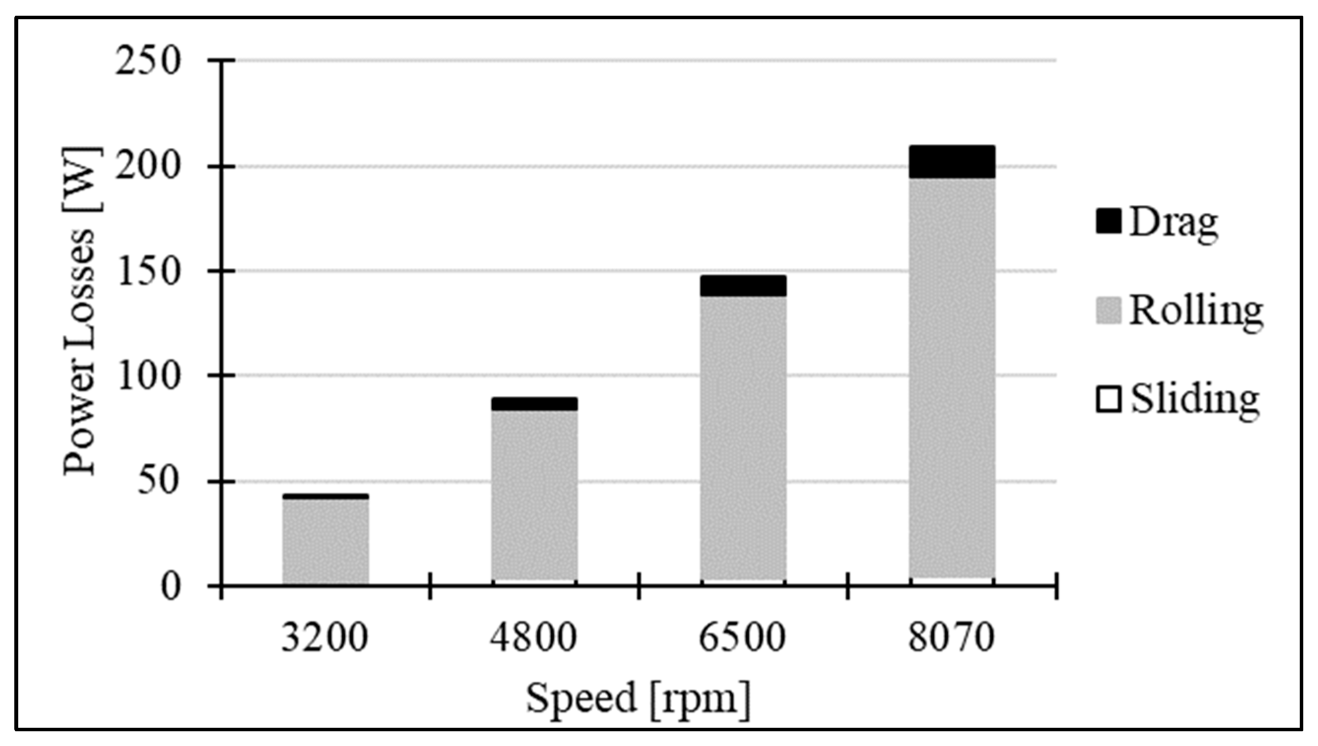
Figure 14a, the model shows a very good agreement with experiments. Speed appears to be correctly taken into account in the model. The power loss distribution at 50 °C is shown in
Figure 15 for different rotational speeds. Hydrodynamic rolling is the major contributor (about 95% of the losses). Sliding is very small (<1%), as well as drag, especially at low speeds.
- -
In
Figure 14b, the influence of the oil temperature injection is similar for the experiments and for the developed model. It emphasizes that the oil temperature which influences power losses is the one at the contact interface between the balls and the rings. This oil temperature is directly related to the temperature of the balls and the rings, and not to the oil injection one.
- -
In
Figure 14c, the calculated power losses are slightly modified by the oil flow rate. The oil flow rate only changes the drag contribution through the intermediary of the oil volume fraction. This fraction modifies the mixture properties, especially its density. Multiplying the oil flow rate by 1.5 leads to an increase of drag losses equal to 16%. However, as shown in
Figure 15, the drag contribution represents only 5% of the total power losses. Therefore, the influence of the oil flow rate is limited. It should be noted that the oil flow is still necessary to avoid starvation effects, which could have an impact on the hydrodynamic rolling contribution.
- -
In
Figure 14d, a good agreement is found between the model and the experiments, especially at high temperatures for a stabilized thermal behavior. One can note a constant increase when the axial preload changes from 225 N to 450 N, whatever the temperature is.
If the influence of speed, preload, oil temperature, and flow rate seem well understood and predicted, the impact of radial load needs a more in-depth analysis.
6.2. Study of the Radial Load Influence
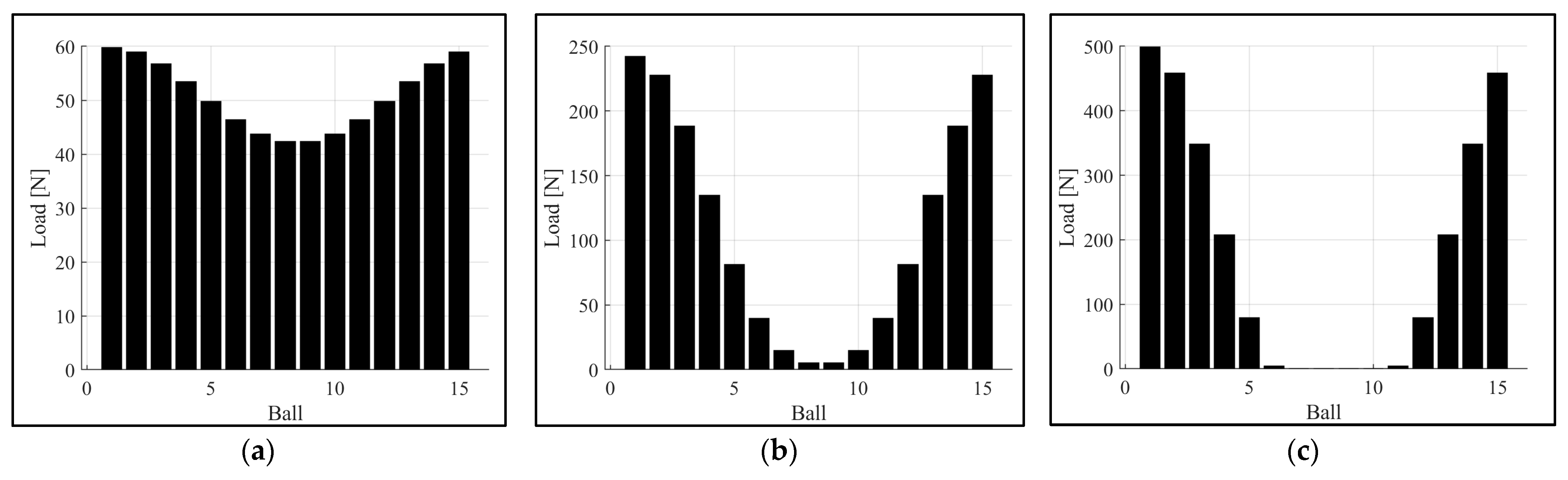
The study of radial load influence is performed on test n°6. The rotational speed is equal to 4800 rpm, the axial preload to 450 N, and three values of the radial load are investigated: 50 N, 650 N, and 1500 N.
First, the load distribution is determined for these different load cases, as shown in
Figure 16:
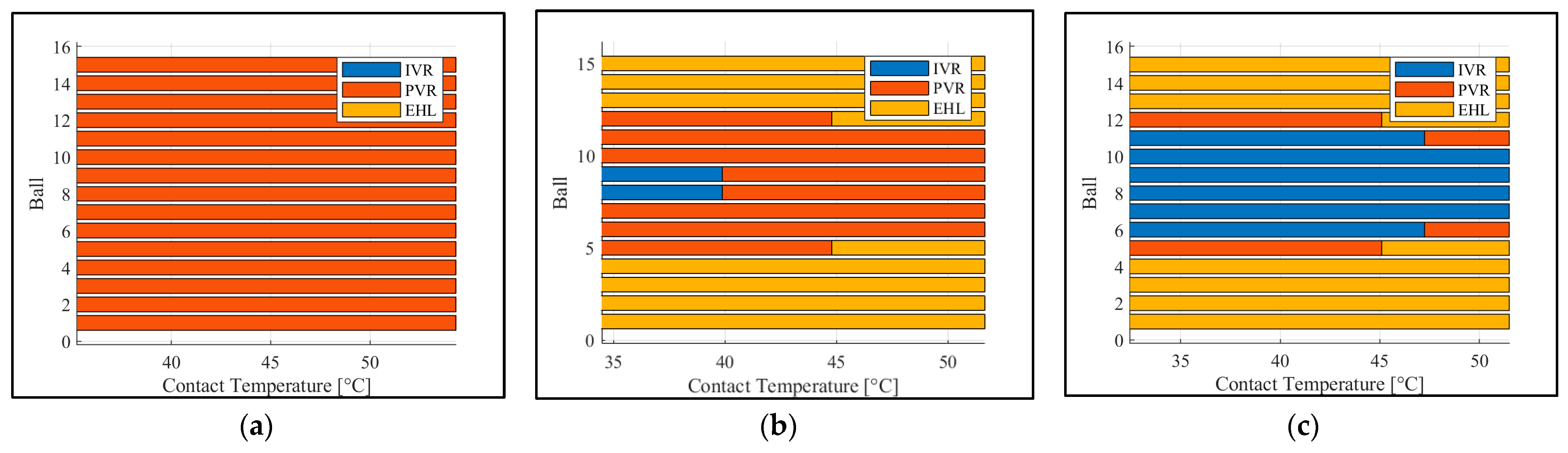
From this distribution and the estimation of the ball temperature through the thermal network, the lubrication regime of each ball is estimated as a function of the contact temperature (see
Figure 17). It can be observed that the PVR regime is present when the contact load is not very high (up to 60 N). Beyond this value, the contact load is sufficient to reach the EHL regime. When the contact load is very low, the IVR regime is found.
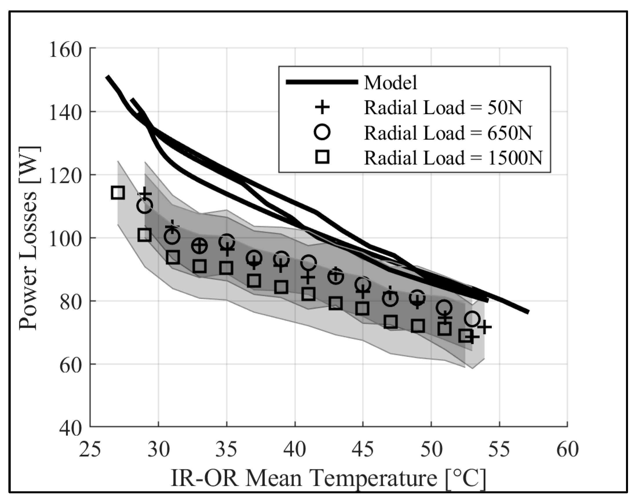
From the regime distribution, the power losses are calculated and compared with measurements. At 4800 rpm,
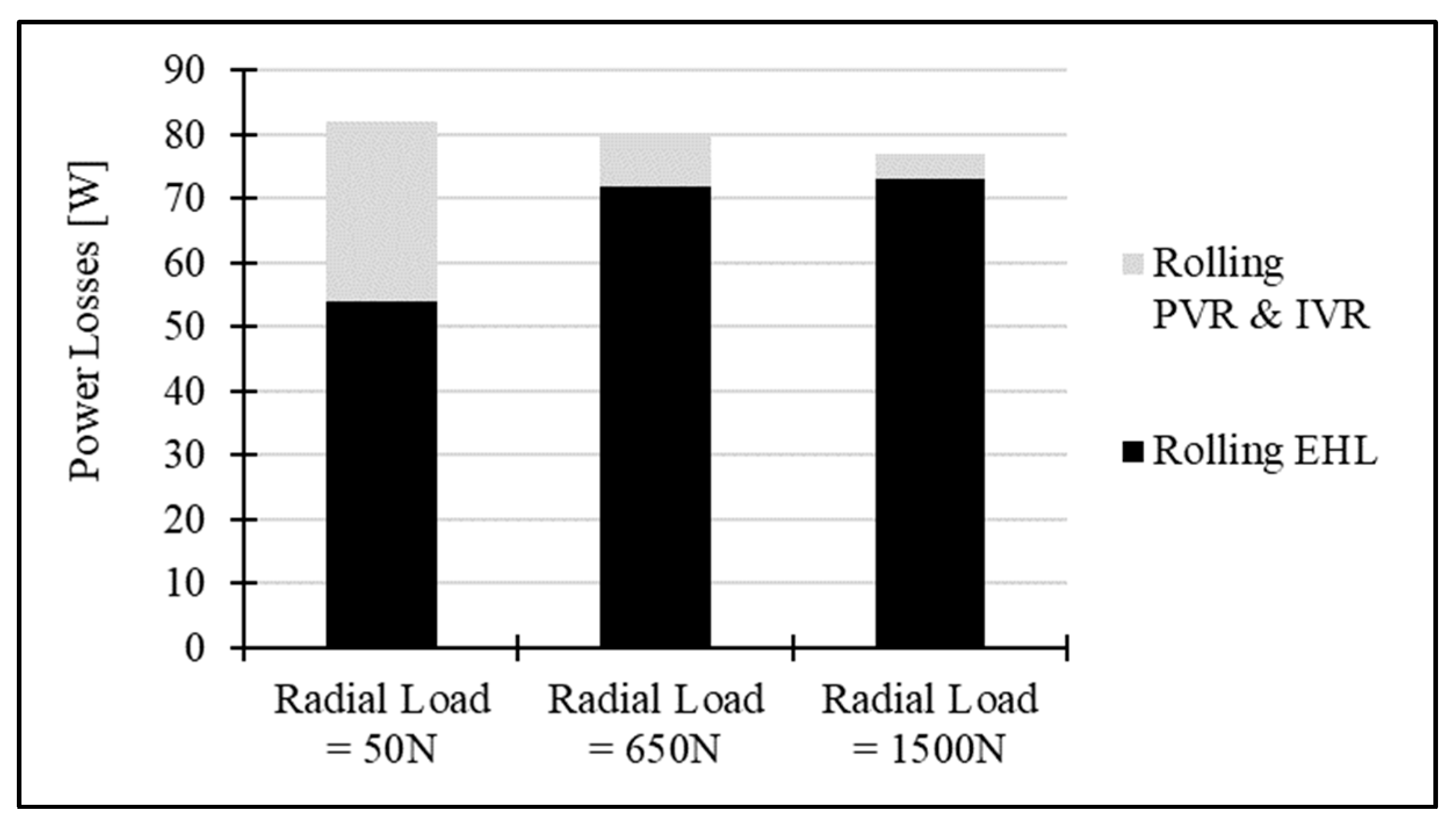
Figure 18 shows that power losses calculated with the model are slightly higher than the measured ones. However, the values are within the measurement uncertainty. Moreover, theoretical calculations confirm that the radial load has almost no influence on power losses (in the tested range). In order to understand the influence of lubrication regime on hydrodynamic rolling power losses,
Figure 19 shows the evolution of hydrodynamic rolling distribution at 50 °C with radial load. In this figure, ‘Rolling EHL’ corresponds to power losses calculated by just considering the EHL regime on all the balls, whereas ‘Rolling PVR & IVR’ corresponds to power losses added by considering the PVR and IVR regimes on low loaded balls. These results highlight that hydrodynamic rolling in the EHL regime decreases as the radial load decreases. But this decrease is compensated by hydrodynamic rolling in PVR & IVR regimes, which leads to an almost constant value of power losses (similar to experimental results).
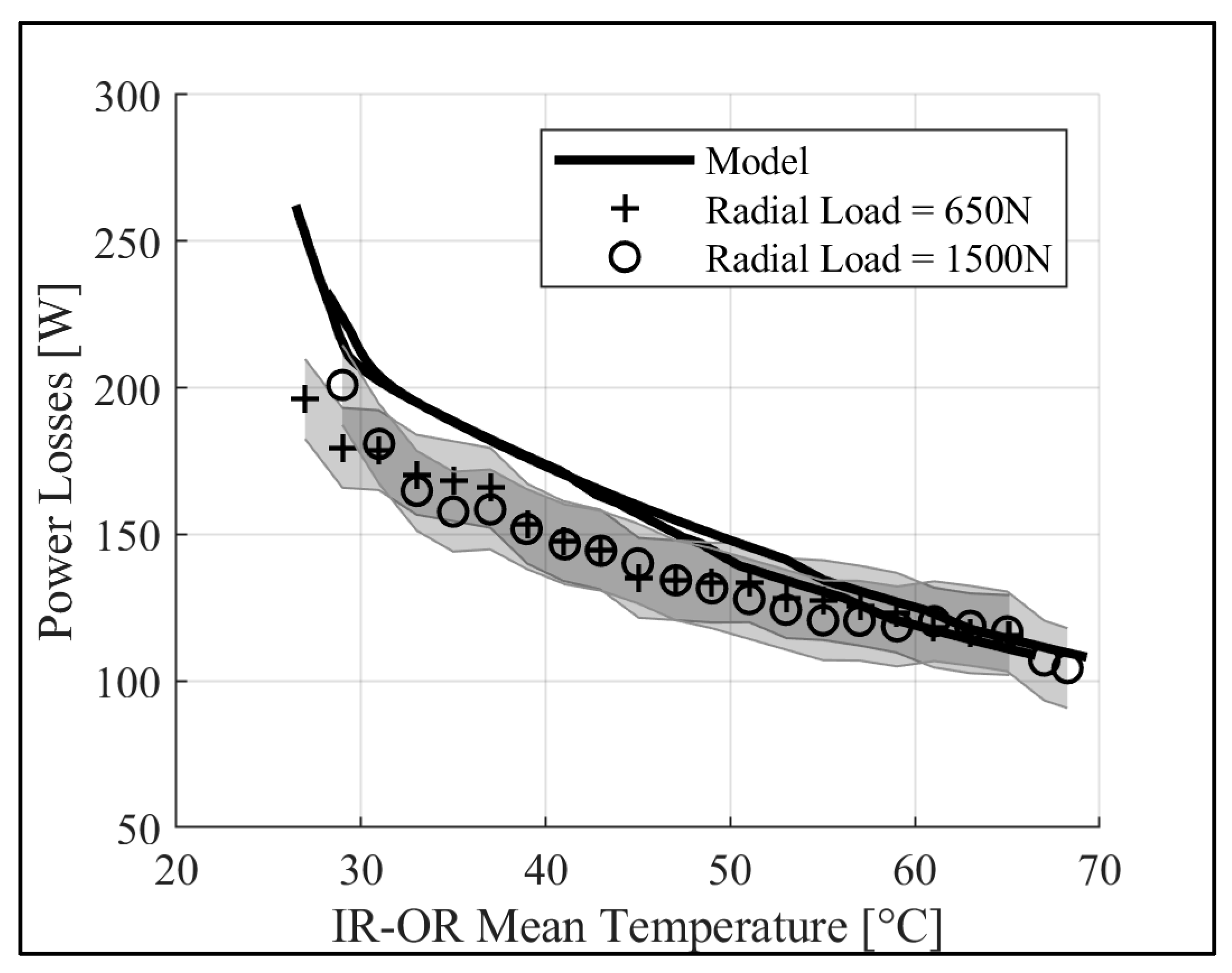
Using the same methodology, the power dissipations were calculated for test n°7 at 6500 rpm and for two radial loads: 650 N and 1500 N. The results are shown in
Figure 20. Once again, the model is perfectly in line with the experiments and confirms the low influence of radial load on power dissipation.
7. Conclusions
A theoretical power loss model is developed for oil-jet-lubricated ACBB. The model is based on a static analysis which gives the load distribution on each ball and accurate information on the contact conditions. Then, the lubrication regime of each rolling element is investigated using Moes’ parameters. It is shown that this lubrication regime can vary from IVR to EHL depending on the loads and contact temperatures. Sliding, hydrodynamic rolling, and drag contributions are calculated at each contact of each ball, resulting in a global power loss generation value. Power losses are injected into a thermal network to account for heat dissipation inside the bearing. The temperature of the balls is calculated and used to estimate the oil viscosity in the contacts. There is therefore a strong coupling between heat generation and heat dissipation, which can affect the lubrication regime.
The model is then compared with measurements. The experimental study is conducted to investigate the influence of several parameters on power losses: rotational speed, oil injection temperature and flow rate, and axial and radial loads. For the range studied, it is shown that speed and axial preload are the two main influential parameters. Surprisingly, the radial load has almost no effect on the power losses. This behavior can be explained by variations associated with the load distribution and the lubrication regime.
As a very good agreement is found between the theoretical model and the measurements, it is highlighted that more than 90% of the power losses are due to the hydrodynamic rolling contribution. Furthermore, the load-independent power losses in ACBB can be explained by the change in the lubrication regime on the contacts.
Author Contributions
Writing—original draft, L.D. Writing—review and editing, C.C., T.T. and F.V. All authors have read and agreed to the published version of the manuscript.
Funding
This research received no external funding.
Data Availability Statement
Data is contained within the article.
Conflicts of Interest
The authors declare no conflicts of interest.
Nomenclature
| ,b | Dimensions of the contact ellipse [m] |
| Distance between raceway groove curvature centers [m] |
| Static capacity [N] |
| Mean diameter [m] |
| Rolling element diameter [m] |
| Equivalent Young’s modulus = [Pa] |
| Osculation = [−] |
| Hydrodynamic rolling force [N] |
| Radial load [N] |
| Axial load [N] |
| Sliding force [N] |
| Dimensionless materials parameter = [−] |
| Dimensionless film thickness [m] |
| Load-deflection factor [ |
| Moes parameters, [] |
| Diametral clearance [m] |
| Power losses, [W] |
| Oil flow rate [] |
| Load on a ball [N] |
| Raceway groove curvature radius [m] |
| , | Equivalent radii [m] |
| Dimensionless speed = [−] |
| Rolling velocity [] |
| Sliding velocity [] |
| Dimensionless load = [−] |
| Z | Number of rolling elements [−] |
| Subscripts | |
| Free contact angle [rad] |
| Contact angle [rad] |
| Pressure–viscosity coefficient [] |
| Coefficient of penetration [−] |
| Geometrical ratio [−] |
| Radii ratio = [−] |
| Curvature sum [] |
| Deflection or contact deformation [m] |
| Dynamic viscosity [] |
| Friction coefficient [−] |
| Location angle of a ball [rad] |
| Rotational speed [] |
| i | Refers to inner ring |
| o | Refers to outer ring |
| j | Refers to ball number |
References
- Zhao, Y.; Zi, Y.; Chen, Z.; Zhang, M.; Zhu, Y.; Yin, J. Power loss investigation of ball bearings considering rolling-sliding contacts. Int. J. Mech. Sci. 2023, 250, 108318. [Google Scholar] [CrossRef]
- Zhou, S.; Singh, A.; Kahraman, A.; Hong, I.; Vedera, K. Power Loss Studies for Rolling Element Bearings Subject to Combined Radial and Axial Loading. SAE Tech. Pap. 2023, 1, 461. [Google Scholar] [CrossRef]
- Wingertszahn, P.; Koch, O.; Maccioni, L.; Concli, F.; Sauer, B. Predicting Friction of Tapered Roller Bearings with Detailed Multi-Body Simulation Models. Lubricants 2023, 11, 369. [Google Scholar] [CrossRef]
- Maccioni, L.; Rüth, L.; Koch, O.; Concli, F. Load-independent power losses of full-flooded lubricated tapered roller bearings: Numerical and experimental investigation of the effect of operating temperature and housing walls distances. Tribol. Trans. 2023, 66, 1078–1094. [Google Scholar] [CrossRef]
- Yilmaz, M.; Lohner, T.; Michaelis, K.; Stahl, K. Bearing Power Losses with Water-Containing Gear Fluids. Lubricants 2020, 8, 5. [Google Scholar] [CrossRef]
- Darul, L.; Touret, T.; Changenet, C.; Ville, F. Power Losses of Oil-Jet Lubricated Ball Bearings with Limited Applied Load: Part 1—Theoretical Analysis. Tribol. Trans. 2023, 66, 801–808. [Google Scholar] [CrossRef]
- Jones, A.B. Ball Motion and Sliding Friction in Ball Bearings. ASME J. Basic Eng. 1959, 81, 1–12. [Google Scholar] [CrossRef]
- Heathcote, H.L. The ball bearing: In the making, under test and on service. Proc. Inst. Automob. Eng. 1920, 15, 569–702. [Google Scholar] [CrossRef]
- Poritsky, H.; Hewlett, C.W., Jr.; Coleman, R.E. Sliding Friction of Ball Bearings of the Pivot Type. ASME J. Appl. Mech. 1947, 14, 261–268. [Google Scholar] [CrossRef]
- Johnson, K.L. The Influence of Elastic Deformation Upon the Motion of a Ball Rolling between Two Surfaces. Proc. Inst. Mech. Eng. 1959, 173, 795–810. [Google Scholar] [CrossRef]
- Tevaarwerk, J.L.; Johnson, K.L. The Influence of Fluid Rheology on the Performance of Traction Drives. ASME J. Technol. 1979, 101, 266–273. [Google Scholar] [CrossRef]
- Houpert, L. Piezoviscous-Rigid Rolling and Sliding Traction Forces, Application: The Rolling Element–Cage Pocket Contact. ASME J. Tribol. 1987, 109, 363–370. [Google Scholar] [CrossRef]
- Zhou, R.S.; Hoeprich, M.R. Torque of Tapered Roller Bearings. ASME J. Tribol. 1991, 113, 590–597. [Google Scholar] [CrossRef]
- Biboulet, N.; Houpert, L. Hydrodynamic Force and Moment in Pure Rolling Lubricated Contacts. Part 1: Line Contacts. Proc. Inst. Mech. Eng. Part J J. Eng. Tribol. 2010, 224, 765–775. [Google Scholar] [CrossRef]
- Pouly, F.; Changenet, C.; Ville, F.; Velex, P.; Damiens, B. Power Loss Predictions in High-Speed Rolling Element Bearings Using Thermal Networks. Tribol. Trans. 2010, 53, 957–967. [Google Scholar] [CrossRef]
- Nelias, D.; Sainsot, P.; Flamand, L. Power Loss of Gearbox Ball Bearing under Axial and Radial Loads. Tribol. Trans. 1994, 37, 83–90. [Google Scholar] [CrossRef]
- Parker, R.J. Comparison of Predicted and Experimental Thermal Performance of Angular Contact Ball Bearings; NASA Technical Paper; NASA: Washington, DC, USA, 1984; Volume 2275, pp. 1–20. [Google Scholar]
- Palmgren, A. Les Roulements: Description, Théorie, Applications, 2nd ed.; SKF Group: Göteborg, Sweden, 1967; 241p. [Google Scholar]
- Harris, T.A. Rolling Bearing Analysis, 3rd ed.; John Wiley and Sons Inc.: New York, NY, USA, 1991; ISBN 0 471 51349 0. [Google Scholar]
- SKF Group. Rolling Bearings; SKF Group: Göteborg, Sweden, 2013; 1375p. [Google Scholar]
- de Cadier de Veauce, F.; Darul, L.; Marchesse, Y.; Touret, T.; Changenet, C.; Ville, F.; Amar, L.; Fossier, C. Power Losses of Oil-Jet Lubricated Ball Bearings With Limited Applied Load: Part 2—Experiments and Model Validation. Tribol. Trans. 2023, 66, 822–831. [Google Scholar] [CrossRef]
- Dindar, A.; Hong, I.; Garg, A.; Kahraman, A. A Methodology to Measure Power Losses of Rolling Element Bearings under Combined Radial and Axial Loading Conditions. Tribol. Trans. 2022, 65, 137–152. [Google Scholar] [CrossRef]
- Brossier, P.; Niel, D.; Changenet, C.; Ville, F.; Belmonte, J. Experimental and Numerical Investigations on Rolling Element Bearing Thermal Behaviour. Proc. Inst. Mech. Eng. Part J J. Eng. Tribol. 2021, 235, 842–853. [Google Scholar] [CrossRef]
- Kerrouche, R.; Dadouche, A.; Mamou, M.; Boukraa, S. Power Loss Estimation and Thermal Analysis of an Aero-Engine Cylindrical Roller Bearing. Tribol. Trans. 2021, 64, 1079–1094. [Google Scholar] [CrossRef]
- Popescu, A.; Olaru, D.N. Influence of lubricant on the friction in an angular contact ball bearing under low load conditions. IOP Conf. Ser. Mater. Sci. Eng. 2020, 724, 12040. [Google Scholar] [CrossRef]
- Bălan, M.R.D.; Houpert, L.; Tufescu, A.; Olaru, D.N. Rolling Friction Torque in Ball-Race Contacts Operating in Mixed Lubrication Conditions. Lubricants 2015, 3, 222–243. [Google Scholar] [CrossRef]
- Moes, H. Optimum similarity analysis with applications to elastohydrodynamic lubrication. Wear 1992, 59, 57–66. [Google Scholar] [CrossRef]
- Dowson, D.; Higginson, G. Elasto-Hydrodynamic Lubrication, SI ed.; Pergamon Press Ltd.: Oxford, UK, 1977; ISBN 9781483181899. [Google Scholar]
- Coulomb, C.A. Théorie des Machines Simples; Bachelier: Paris, France, 1821; 387p. [Google Scholar]
- Houpert, L. Hydrodynamic Load Calculation in Rolling Element Bearings. Tribol. Trans. 2016, 59, 538–559. [Google Scholar] [CrossRef]
- Biboulet, N.; Houpert, L. Hydrodynamic Force and Moment in Pure Rolling Lubricated Contacts. Part 2: Point Contacts. Proc. Inst. Mech. Eng. Part J J. Eng. Tribol. 2010, 224, 777–787. [Google Scholar] [CrossRef]
Figure 1.
(a) Free contact angle. (b) Ball location and applied loads.
Figure 1.
(a) Free contact angle. (b) Ball location and applied loads.
Figure 2.
Load distribution on each ball. (a) DGBB Fr = 1 kN. (b) ACBB Fa = 400 N.
Figure 2.
Load distribution on each ball. (a) DGBB Fr = 1 kN. (b) ACBB Fa = 400 N.
Figure 3.
Mapping the lubrication regime. (a) Moes − Deep groove ball bearing (DGBB) − Fr = 1 kN (b) Moes − Angular contact ball bearing (ACBB) − Fa = 400 N. (c) Regime evolution of each ball for DGBB. (d) Regime evolution of each ball for ACBB.
Figure 3.
Mapping the lubrication regime. (a) Moes − Deep groove ball bearing (DGBB) − Fr = 1 kN (b) Moes − Angular contact ball bearing (ACBB) − Fa = 400 N. (c) Regime evolution of each ball for DGBB. (d) Regime evolution of each ball for ACBB.
Figure 4.
Diagram of power loss calculation.
Figure 4.
Diagram of power loss calculation.
Figure 5.
Thermal network of a bearing.
Figure 5.
Thermal network of a bearing.
Figure 6.
Test rig architecture.
Figure 6.
Test rig architecture.
Figure 7.
Visualization of the test rig.
Figure 7.
Visualization of the test rig.
Figure 8.
Evolution of inner ring (IR) temperature for 4 different speeds.
Figure 8.
Evolution of inner ring (IR) temperature for 4 different speeds.
Figure 9.
(a) Evolution of power losses for 4 different speeds with respect to time. (b) Evolution of power losses for 4 different speeds with respect to outer ring (OR)–inner ring (IR) mean temperature.
Figure 9.
(a) Evolution of power losses for 4 different speeds with respect to time. (b) Evolution of power losses for 4 different speeds with respect to outer ring (OR)–inner ring (IR) mean temperature.
Figure 10.
Evolution of power losses for 2 different oil injection temperatures with respect to OR-IR mean temperature.
Figure 10.
Evolution of power losses for 2 different oil injection temperatures with respect to OR-IR mean temperature.
Figure 11.
Evolution of power losses for 2 different oil flow rates with respect to OR-IR mean temperature.
Figure 11.
Evolution of power losses for 2 different oil flow rates with respect to OR-IR mean temperature.
Figure 12.
Evolution of power losses for different axial preloads with respect to OR-IR mean temperature: (a) 4800 rpm, (b) 6500 rpm.
Figure 12.
Evolution of power losses for different axial preloads with respect to OR-IR mean temperature: (a) 4800 rpm, (b) 6500 rpm.
Figure 13.
Evolution of power losses for different radial loads with respect to OR-IR mean temperature: (a) 4800 rpm, (b) 6500 rpm.
Figure 13.
Evolution of power losses for different radial loads with respect to OR-IR mean temperature: (a) 4800 rpm, (b) 6500 rpm.
Figure 14.
Comparison between model and experiments for the different parameters investigated. (a) Influence of speed (b) Influence of oil injection temperature. (c) Influence of oil flow rate. (d) Influence of axial preload.
Figure 14.
Comparison between model and experiments for the different parameters investigated. (a) Influence of speed (b) Influence of oil injection temperature. (c) Influence of oil flow rate. (d) Influence of axial preload.
Figure 15.
Power loss distribution for different speeds.
Figure 15.
Power loss distribution for different speeds.
Figure 16.
Load distribution for 3 load cases. (a) Radial load = 50 N. (b) Radial load = 650 N. (c) Radial load = 1500 N.
Figure 16.
Load distribution for 3 load cases. (a) Radial load = 50 N. (b) Radial load = 650 N. (c) Radial load = 1500 N.
Figure 17.
Regime lubrication of each ball for 3 load cases. (a) Radial load = 50 N. (b) Radial load = 650 N. (c) Radial load = 1500 N.
Figure 17.
Regime lubrication of each ball for 3 load cases. (a) Radial load = 50 N. (b) Radial load = 650 N. (c) Radial load = 1500 N.
Figure 18.
Comparison between model and experiments for three different radial loads, speed = 4800 rpm.
Figure 18.
Comparison between model and experiments for three different radial loads, speed = 4800 rpm.
Figure 19.
Hydrodynamic rolling distribution, at 50 °C, for three different radial loads, speed = 4800 rpm.
Figure 19.
Hydrodynamic rolling distribution, at 50 °C, for three different radial loads, speed = 4800 rpm.
Figure 20.
Comparison between model and experiments for two different radial loads, speed = 6500 rpm.
Figure 20.
Comparison between model and experiments for two different radial loads, speed = 6500 rpm.
Table 1.
Bearing characteristics.
Table 1.
Bearing characteristics.
| Characteristics | DGBB | ACBB |
|---|
| Reference | 6210Z | 7210 |
| Mean diameter (mm) | 70 | 70 |
| Outer diameter (mm) | 90 | 90 |
| Bore diameter (mm) | 50 | 50 |
| Free contact angle (°) | 0 | 40 |
| Width (mm) | 20 | 20 |
| Number of balls (−) | 10 | 15 |
Table 2.
Steel properties.
Table 2.
Steel properties.
| Characteristics | Value |
|---|
| Young modulus (GPa) | 210 |
| Poisson coefficient (−) | 0.3 |
Table 3.
Oil properties.
| Characteristics | Value |
|---|
| Kinematic viscosity at 40 °C (cSt) | 36.6 |
| Kinematic viscosity at 100 °C (cSt) | 7.8 |
| Density at 15 °C (kg.m−3) | 864.6 |
| Pressure–viscosity coefficient (Pa−1) | |
Table 4.
Test matrix for 7210 ACBB.
Table 4.
Test matrix for 7210 ACBB.
| Test n° | Speed
(rpm) | Oil Inj. T°
(°C) | Oil Flow Rate
(L/h) | Axial Preload
(N) | Radial Load
(N) |
|---|
| 1 | Four points | 30 °C | 10 | 450 | 650 |
| 2 | 6500 | Two points | 10 | 450 | 650 |
| 3 | 8070 | 30 °C | Two points | 450 | 650 |
| 4 | 4800 | 30 °C | 10 | Three points | 0 |
| 5 | 6500 | 30 °C | 10 | Two points | 650 |
| 6 | 4800 | 30 °C | 10 | 450 | Three Points |
| 7 | 6500 | 30 °C | 10 | 450 | Two Points |
| Disclaimer/Publisher’s Note: The statements, opinions and data contained in all publications are solely those of the individual author(s) and contributor(s) and not of MDPI and/or the editor(s). MDPI and/or the editor(s) disclaim responsibility for any injury to people or property resulting from any ideas, methods, instructions or products referred to in the content. |
© 2024 by the authors. Licensee MDPI, Basel, Switzerland. This article is an open access article distributed under the terms and conditions of the Creative Commons Attribution (CC BY) license (https://creativecommons.org/licenses/by/4.0/).


