1. Introduction
Under normal operating conditions, a reasonably designed sliding bearing is considered to work under full film lubrication, and the friction surfaces are completely separated by the lubrication film. The film thickness ranges from a few microns to tens of microns, depending on the type of bearing, operating conditions and lubricant. In practice, the sliding surfaces cannot be completely smooth due to manufacturing defects. The manufacturing error or surface roughness is more obvious when machining large-size or polymer bearings. Especially for water-lubricated bearings, the low viscosity of water and the weak bearing capacity of the water film make the contact friction between the asperities inevitable under starting, low speed, heavy load and other working conditions [
1]. In these cases, the bearing is actually in a mixed lubrication state.
An elastic rubber support water-lubricated tilting pad thrust bearing (RWTB) performs excellently in vibration reduction and load sharing and is thus applied to underwater vehicle thrusters with high requirements for concealment [
2]. In a previous study [
3], a thermo-elasto-hydrodynamic (TEHD) lubrication performance model of the RWTB bearing was established, based on which the bearing structure was optimized. However, in practical applications, the abnormal wear of the RWTB bearing occurred many times, which may be attributed to the great impact of the surface roughness of bearing friction surfaces on the lubrication performance. The TEHD model does not take into account the influence of roughness on bearing lubrication performance, which results in the unsatisfactory optimized bearing structure, making it necessary to establish a mixed lubrication model of the RWTB and carry out the bearing structure optimization based on the mixed lubrication model.
Take into account the influence of roughness on the lubrication state, and consider the contact of asperities as the iconic feature of mixed lubrication. According to the manifestation of surface roughness in the mixed lubrication analysis model, the mixed lubrication model can be divided into two types, i.e., the statistical model and the deterministic model. The former is based on the Reynolds equation, in which several parameters representing the macroscopic characteristics of surface roughness are introduced, but the actual surface roughness distribution is not directly included in the film thickness expression, and the local asperity contact is not really considered. A representative study is the average Reynolds equation model (also known as the PC flow model) proposed by Patir and Cheng et al. [
4,
5], which is characterized by the use of pressure flow factors and shear flow factors containing macroscopic characteristic parameters of roughness to modify the Reynolds equation. The latter is also based on the Reynolds equation, in which the actual height of surface roughness is directly included in the film thickness expression, and the local asperity contact is considered in the calculation process. The most innovative work is the unified Reynolds equation model proposed by Zhu and Hu [
6,
7], which solves the fluid lubrication problem and the micro-convex contact problem using a unified model.
The average Reynolds equation model is still widely used as an effective method to analyze the mixed lubrication performance under two-dimensional roughness [
8,
9]. The core of the model is the calculation of the pressure flow factor and the shear flow factor. Elrod [
10] dealt with the pressure term in the Reynolds equation and solved the flow factor through a Fourier transform using the perturbation expansion method. Moreover, the calculation results were compared with the results of the average Reynolds equation model, and it was pointed out that the flow factor calculation method of the latter ignored the non-diagonal term in the flow factor tensor. Tripp [
11] solved the flow factor based on Elrod’s work and combined it with Green’s function method, which is in good agreement with Elrod’s calculation results. Peeken et al. [
12] improved the calculation method of the flow factor, and compared it with the results of Elrod and Tripp. It was found that the flow factor obtained by the analytical method and the numerical method was significantly different under the skewed surface. Given that the increase in the local contact area is accompanied by the decrease in the accuracy of the model, elastoplastic deformation is not considered in the average Reynolds equation model when h/σ < 0.5 (h is the film thickness, and σ is the root mean square of roughness). Kim et al. [
13] applied a numerical method for calculating the flow factor of the average Reynolds equation model considering elastic deformation. Harp et al. [
14] proposed a flow factor calculation method, with the cavitation effect between micro-convex bodies taken into account.
Because the statistical model uses the concept of average in the actual film thickness and pressure treatment, the use of the concepts of “average” and “statistics” determines that it cannot accurately describe the real situation of rough surfaces as the mixed lubrication deterministic model does, although it can solve the mixed lubrication performance parameters such as the nominal film thickness, friction work and bearing capacity. Chang et al. [
15,
16] studied the fracture of the elastohydrodynamic lubrication film through the deterministic thermal transient model, introduced the local asperity contact into the deterministic model analysis, and proposed the concept of partial elastohydrodynamic lubrication. For the problem of the line contact, the nominal contact is divided into the micro-convex contact area and the fluid lubrication area. The contact area and contact stress in the contact area are solved by the contact theory, while the actual height of roughness is included in the film thickness expression in the fluid area and the pressure distribution is directly solved by using the Reynolds equation. Ai et al. [
17,
18] first established a full numerical transient model of point contact mixed lubrication considering surface roughness using the measured surface roughness data of the point contact area of rolling bearings. Jiang [
19] further developed the partial elastohydrodynamic lubrication model for point contact problems using the FFT inverse algorithm and the multigrid method to solve the contact pressure of asperities in the contact area and the liquid film pressure in the fluid area, thus improving the calculation efficiency. On this basis, Zhu and Hu [
6,
7] proposed a unified Reynolds equation model and developed a program package for calculating the point contact partial elastohydrodynamic lubrication performance of ball bearings. The model divides the lubrication area into two parts, i.e., the fluid lubrication area and the contact area. The Reynolds equation is used to solve the dynamic pressure in the lubrication zone. In the contact region, the Reynolds equation is reduced to the form of
, which is used to solve the contact pressure. The numerical examples indicate the simpleness and reliability of the unified Reynolds equation model and the new numerical method, which can also deal with three-dimensional rough surface lubrication problems at different rolling and sliding speeds. For full film lubrication, mixed lubrication and boundary lubrication, a unified numerical program can be used for obtaining complete numerical solutions. Wang et al. [
20] established a point contact thermal elastohydrodynamic transient mixed lubrication model based on the unified Reynolds equation model, and conducted a transition study from full liquid film lubrication to boundary lubrication using an improved elastic deformation algorithm based on discrete convolution and FFT transform. Moreover, in order to reduce the solution error and improve the solution speed, Li et al. [
21] studied the point contact mixed lubrication problem based on the unified Reynolds equation model using the asymmetric control volume dispersion method. The point contact mixed lubrication performance results [
6,
18,
20] calculated by the unified Reynolds equation model are in good agreement with the test results [
22,
23], which provides a reliable solution to the point contact mixed lubrication problem of non-conformal surfaces.
Regarding the aspect of mixed lubrication of conformal surfaces, Dobrica et al. [
24,
25] successively studied the mixed elastohydrodynamic lubrication performance of radial sliding bearings and the influence of elastoplastic deformation of micro-convex contact on the lubrication performance using a deterministic model, and compared the calculation results with those of the statistical model. Ignoring the elastic deformation, the transverse roughness (perpendicular to the fluid flow direction) has the greatest influence on the lubrication performance. The average film thickness and friction torque are increased by 30% and 54%, respectively, compared with those without considering the roughness. However, when elastic deformation is taken into account, they are reduced to 8% and 25%, respectively. Given that the statistical model does not consider the actual asperity contact, its calculation accuracy is acceptable under low and medium load conditions. In addition to the research of Dobrica et al., the deterministic model is rarely applied to the study of mixed lubrication problems on conformal surfaces such as sliding bearings as well as the analysis of multi field coupling problems closely related to engineering practice. The main reason is that, compared with the point contact problem, the sliding bearing may be in surface contact at the stage of heavy load and low speed. In order to truly simulate the influence of roughness, the computational domain must be divided into a high-density discrete grid, indicating the necessity of advanced algorithms and computer hardware. Taking the study of Dobrica et al. [
25] as an example, the surface of the small bearing bush with 19.84 mm × 17.92 mm is divided into 1984 × 1792 rectangular grid elements with 3.6 million nodes. Only one iteration of deformation solution requires 46 TB of computer storage space and 12.6 × 10¹² times of multiplication, which is almost impossible for an ordinary computer. For this reason, according to the different influence degrees of the pressure acting point and the node spacing to calculate the deformation on the deformation, the grid division method of thick and thin density was skillfully adopted in the case of calculating the deformation influence coefficient matrix, which improved the calculation efficiency by 400 times without affecting the accuracy. Moreover, Xiong et al. [
26] also made an in-depth study on this elastic deformation algorithm, which only calculated and stored the deformation influence coefficient in a small area near the pressure point, providing an effective calculation method for the simulation of transient contact elastohydrodynamic lubrication performance by combining with the local fine-mesh generation technology.
In this paper, in order to more realistically simulate the influence of surface roughness on the performance of the RWTB, and to better optimize the bearing structure, efforts are made to establish a deterministic mixed lubrication model of the RWTB, which incorporates the elastic–plastic deformation of asperities and the polymer matrix materials, friction heat and elastic deformation of the rubber support. The lubrication performance calculated by the ML model is then compared with the results simulated by the THD model and the TEHD model [
3], and the film thickness is also compared with the measurements [
27].
2. Bearing Structure and the Mixed Lubrication Model
2.1. Structure of the RWTB
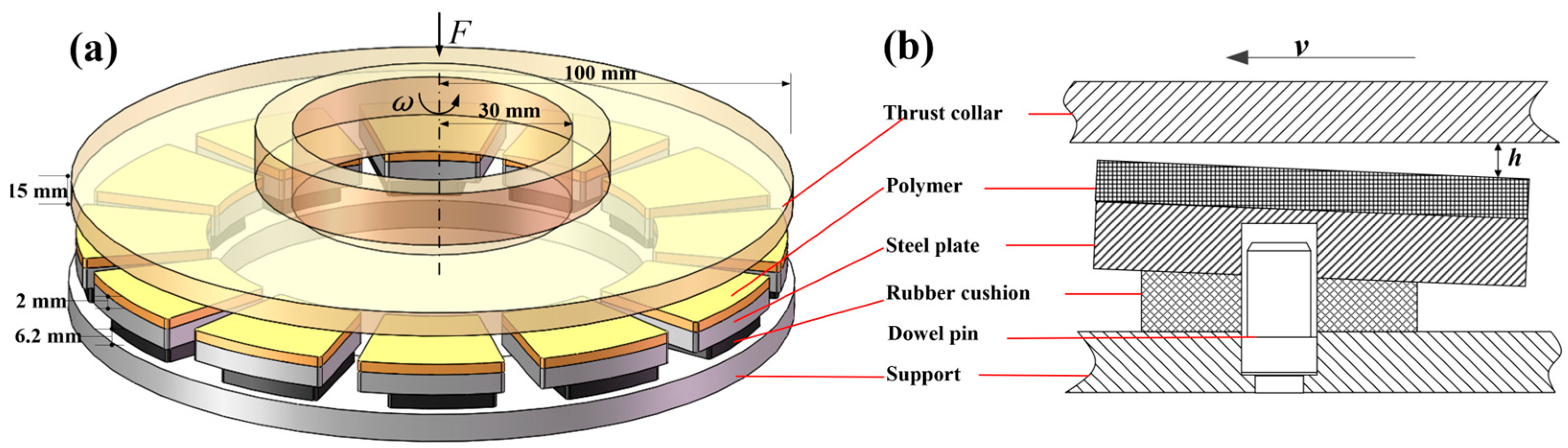
The structure, material and dimension parameters of the RWTB are the same as those in Reference [
3], and the bearing is shown in
Figure 1. It is mainly composed of a thrust collar, several thrust pads and a support ring, wherein each thrust pad consists of a polymer pad surface, a steel pad plate and a rubber cushion. Dowel pins installed on the support ring are used to locate the thrust pads, which can only be tilted but cannot be moved. The rubber cushion is offset at the bottom of the steel plate, which makes the thrust pad tilt adaptively under different working conditions. Moreover, the elasticity of the rubber can improve the load-sharing capacity of the bearing pads under the inclined shaft state, as well as the level of vibration and noise reduction under bad working conditions. During operation, the thrust collar rotates and transmits the axial force to each pad. A water film will be formed between the thrust collar and each polymer pad surface. In the case of bearing in the mixed lubrication state, the water film force and the micro-asperities contact force between the friction surfaces will jointly bear the axial force from the thrust collar.
2.2. Mathematical Model of Surface Roughness with Random Distribution
The commonly used mathematical characterization methods of roughness mainly include the direct measurement method, the statistical parameter method and the mathematical model generation method. The statistical method [
28] describes the surface macroscopic morphology characteristics through the statistical parameters of rough surfaces, the roughness height distribution function and the characteristics of the distribution function. Parameters including standard deviation of roughness height distribution, roughness density per unit area, radius of curvature of roughness, etc. are generally involved. The mathematical model generation method [
29] is based on the measured characteristic parameters of the roughness, and generates the sine (cosine) or random roughness conforming to Gaussian or non-Gaussian distribution with the same characteristic parameters as the measurement results using mathematical equations.
The surface profile of the thrust pad polymer surface is measured by a laser interference surface-topography-measuring instrument [
27]. The distribution feature of surface roughness is Gaussian distribution. Hence, the surface roughness model proposed by Patir [
4] is used for the generation of the surface roughness profile. The essence of this model is to first grid the surface and the autocorrelation length, then generate a random number matrix
η with a mean value of 0 and a standard deviation of 1 that conforms to the Gaussian distribution using a random number generator based on the number of grids, and then solve the autocorrelation coefficient matrix
R. Finally, the surface roughness matrix is generated by linear transformation of the random number matrix and the autocorrelation coefficient matrix.
First, the rough surface and the autocorrelation length
are divided into grids along the
x and
y axis directions to generate
N × M and
n × m nodes, respectively, and a random number matrix
η of order
(N + n) × (M + m) is generated using Matlab. The elements of the autocorrelation coefficient matrix calculated by the autocorrelation function formula are:
where
The matrix
a can be solved by the Newton iteration method, which can be expressed as:
where
The calculation method of each element in the Jacobian matrix
J can be expressed as:
where
The initial value of the element of matrix
a is:
where
Thus, each element of matrix
a in the expression (2) of each element of the autocorrelation coefficient matrix
R can be obtained, and the roughness height at each node of the surface can then be obtained as:
where
Different roughness distributions can be obtained by changing the root mean square of surface roughness,
Sq, and the autocorrelation length,
.
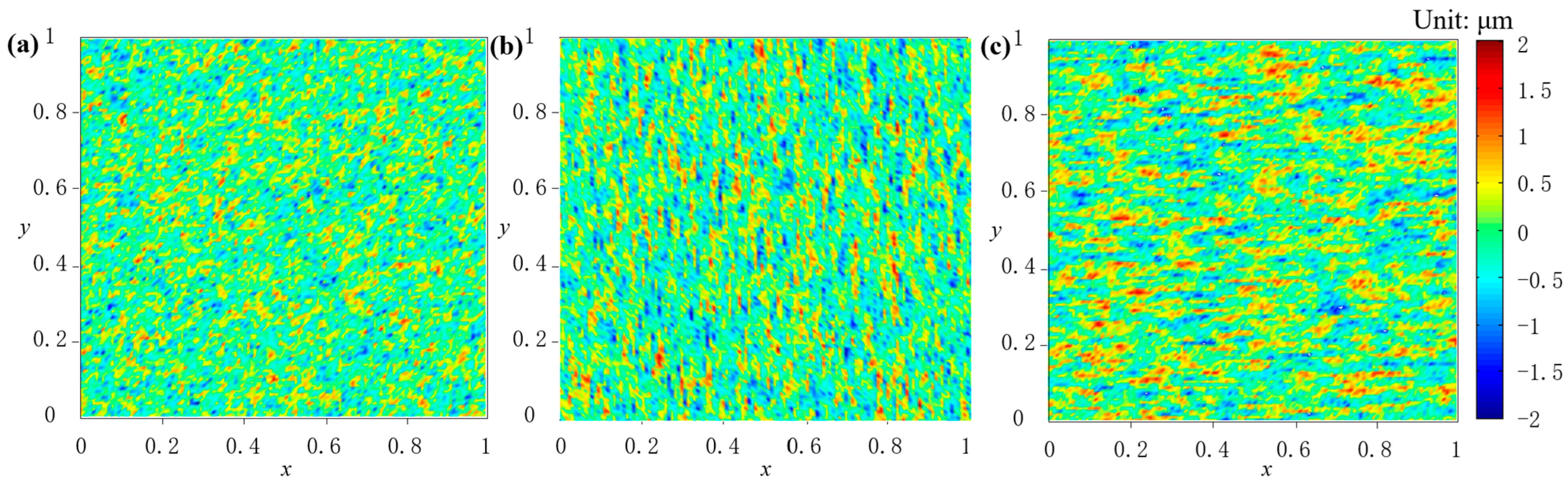
Sq is set to 0.5 μm, the autocorrelation length ratio λ is set to 1, 1/4 and 4, respectively, and the obtained surface roughness distribution is shown in
Figure 2. The roughness distribution in
Figure 2a is close to isotropy, while the roughness in
Figure 2b tends to be distributed along the vertical direction and that in
Figure 2c tends to be distributed along the horizontal direction. This means that in the case of different λ values, the generated surface roughness can be distributed while presenting directional characteristics. If the fluid flows through the surface in
Figure 2 in a horizontal direction, it can be obviously observed that the three types of roughness will have different effects on the fluid velocity and hydrodynamic pressure.
2.3. Contact and Deformation Model of Micro-Asperities
In terms of contact modeling and calculation methods, the micro-asperity elastic contact model (GW model) proposed by Greenwood and Williamson [
28] is the most widely used. The micro-asperities are assumed to be hemispherical, and the curvature radii of the hemispheres are equal. According to the Hertz contact theory, the micro-asperity is subjected to elastic deformation under the contact pressure of a rigid plane. Contact radius
a, contact area
A and contact force
F can be respectively expressed as:
where
δa denotes the elastic deformation of the micro-asperity;
Ea, the effective elastic modulus of the micro-asperity material;
Ea =
E1/(1 −
v12);
E1, the elastic modulus of the micro-asperity material;
v1, the Poisson’s ratio; and
R, the curvature radii of the hemisphere. The contact force F refers to the normal force between the micro-asperity and the flat plate.
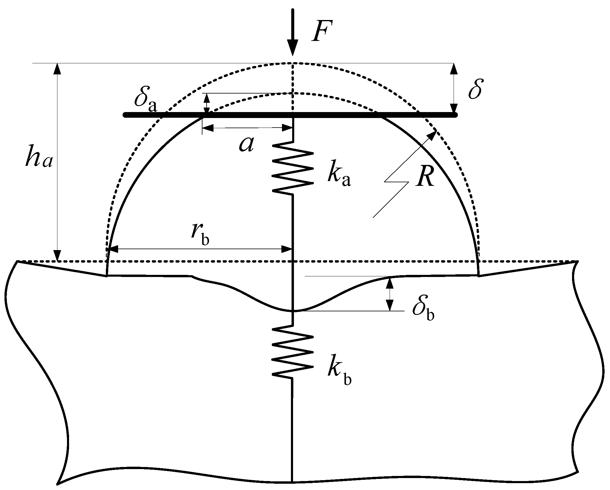
However, the GW model only considers the contact deformation of the asperities, not taking into account the deformation of the matrix material where the asperities are located. On the basis of the above theory, Yeo et al. [
30] proposed a contact deformation model of a micro-asperity considering the deformation of the elastic matrix material. The principle of this model is shown in
Figure 3.
When the asperity is deformed by the contact force, the elastic matrix material at the bottom of the asperity will also be deformed correspondingly. The total deformation is equal to the sum of the both deformations. If the micro-asperity and the matrix are regarded as two springs in series, and the total stiffness is
k, then:
Yeo et al. [
30] regarded the matrix material as a half-infinite space body, deduced the relationship between the matrix deformation and the asperity contact pressure, and further deduced that between the deformation of the micro-asperity and the total deformation.
The matrix material actually has a certain thickness and is not a half-infinite space body. Therefore, the stiffness of the matrix material calculated by using the half-infinite space body will be less than the actual value. The thickness of the polymer layer of the thrust pad is 2 mm, far less than its length and width, so it can be regarded as a thin plate. By using the thin plate deformation model [
31], in the circular area with radius
rb, the normal displacement of the substrate surface can be expressed as:
where,
t,
E2 and
v2 are the thickness, elastic modulus and Poisson’s ratio of the matrix material, respectively, and
.
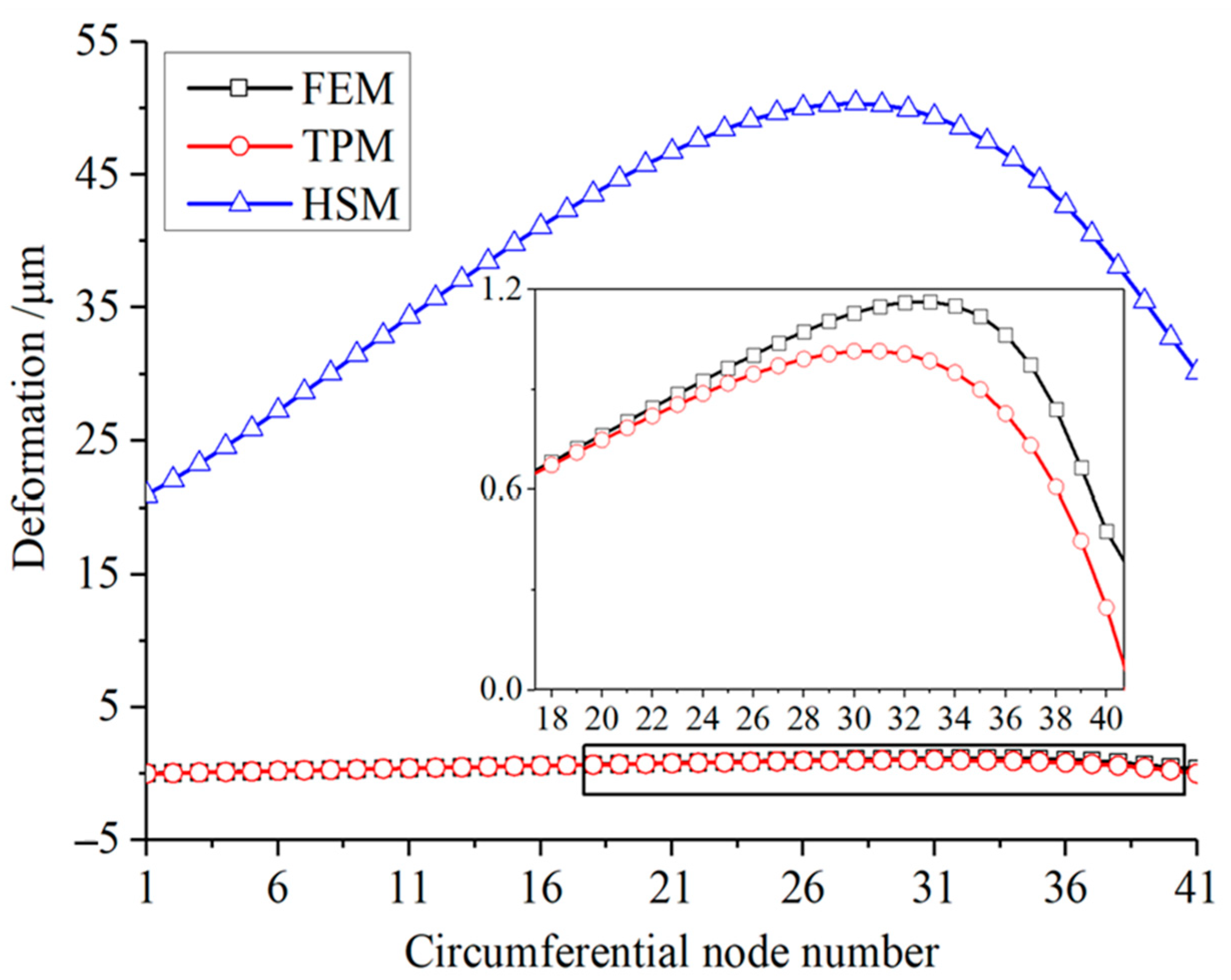
The half-infinite space model (HSM), the finite element model (FEM) and the thin plate deformation model (TPM) are jointly used to calculate the deformation of the polymer material of the thrust pad. Under the rated working condition (the specific pressure is 0.5 MPa), the water film pressure distribution of the bearing calculated by a THD model is respectively substituted into the above deformation models. The comparison of the calculated elastic deformation results at the average radius of the pad is shown in
Figure 4.
As shown in
Figure 4, the HSM model has seriously overestimated the deformation, while the results calculated by the FEM and TPM model are in good agreement. Therefore, the TPM model, instead of the HSM model, is hereby used to calculate the contact deformation of the matrix material, which can not only improve the accuracy of the deformation calculation, but also reduce the solution time compared with the FEM model.
Substituting Equations (6) and (9) into Equation (7), the deformation relationship can be obtained after taking into account the thickness of the matrix material:
The micro-asperities and the matrix of the polymer material are usually the same material. Therefore, their elastic modulus and Poisson’s ratio are equal, and Formula (10) can thus be further simplified as:
The above formula can be further simplified into an iterative form similar to Equation (15) in Reference [
30] to solve the deformation
δa of micro-asperities. Further, the contact area A and contact force F of the asperities are solved. Moreover, it should be emphasized that the yield limit of the polymer material selected in this paper is 37.5 MPa. The calculation shows that when the contact deformation of the micro-asperity exceeds one thousandth of its curvature radius, the contact stress of the material will reach the yield limit. In this case, when the compression continues to increase, the elasto-plastic theory [
32] should be used to calculate the contact area and contact force, when the contact pressure is considered the yield limit of the material, which does not increase with the increase in compression.
2.4. Deterministic Model of Mixed Lubrication
In the mixed lubrication deterministic model, considering the possible existence of micro-convex contact between the pad surface and the thrust collar, the pad surface should be divided into two areas, i.e., the fluid lubrication area Ω
f and the solid contact friction area Ω
c. In the fluid lubrication zone, the two surfaces are completely separated by the water film. Although there are micro-asperities interfering with the water film flow, they will not completely block the flow. The local contact area only accounts for a small part of the total area of the pad, so the Reynolds equation is still considered applicable for solving the water film pressure distribution in this area [
6].
The boundary conditions of the Reynolds Equation (12) are:
, if
p < 0,
p = 0.
is the boundary of the thrust pad. In the contact area of micro-asperities, the thickness of water film is 0, and the contact area and contact force can be solved by the elastic contact model of micro-asperities proposed in
Section 2.3. When the contact pressure exceeds the material compression yield limit, the contact pressure will be equal to the yield limit.
In order to solve the fluid pressure near the edge of the contact area of the micro-asperity , the water film pressure at the edge of the contact area of the micro-asperity is assumed to be equal to the average contact pressure ; that is, when , .
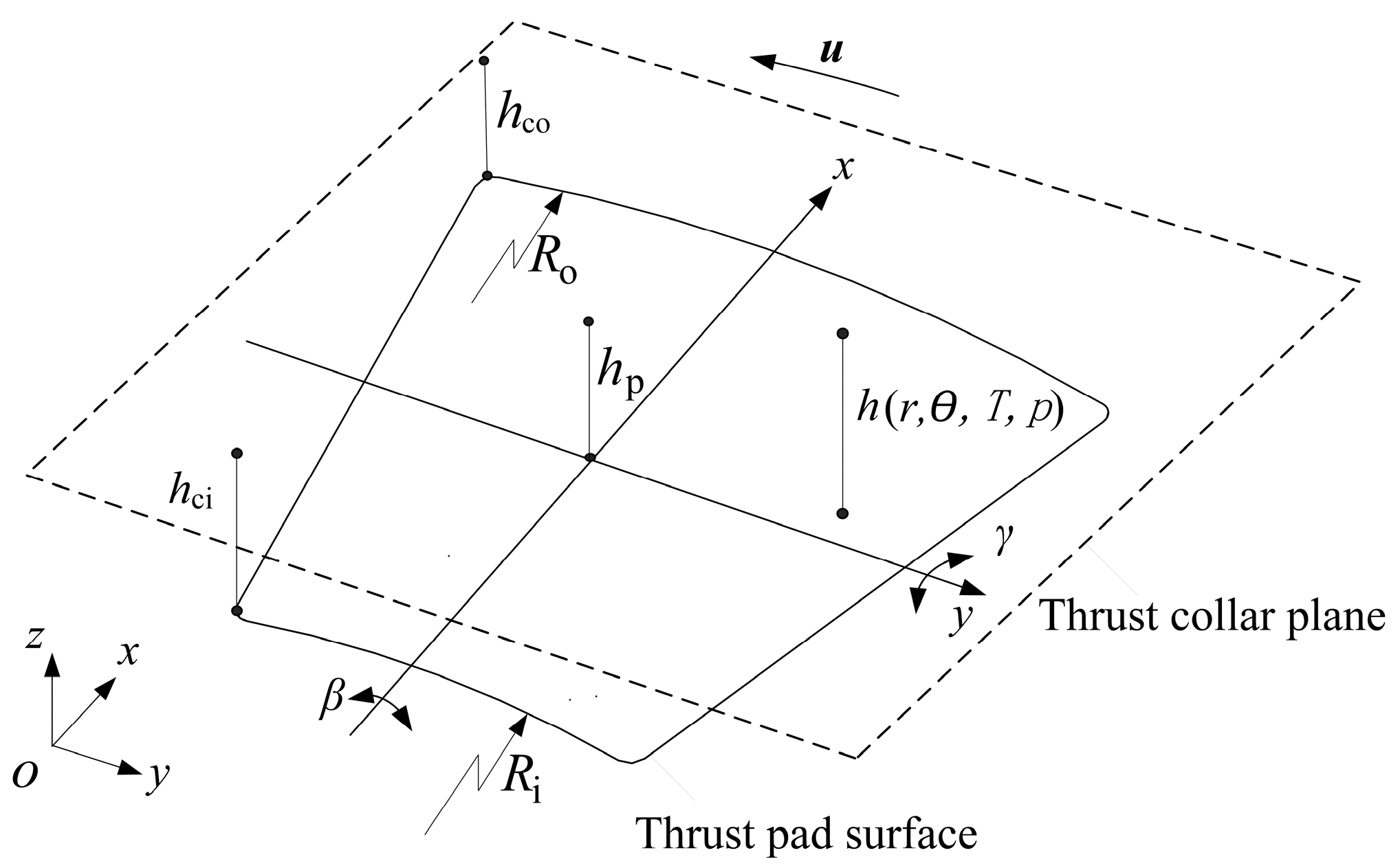
In the mixed lubrication model, there may exist solid contact, and the contact point may first appear near the two vertices at the water film outlet side of the pad. Therefore, the film thickness expression is rewritten by taking the water film outlet side vertex as the reference point, with the influence of surface roughness on the film thickness included. At this time, the film thickness can be expressed as:
where
represents the height of the micro-convex body;
, the film thickness at the vertices of the water film outlet side, which is determined according to the tile inclination;
θ, the circumferential angle of the thrust pad; and
θe, the circumferential angle of the
x axial (circumferential angle of the symmetry axis of the rubber cushion). The thickness of the water film on the pad and pad surface is shown in
Figure 5.
And if
, then:
where
and
are the inner and outer radii of the pad, respectively. Taking the film thickness at the vertices of the outlet side as the reference point to calculate the film thickness distribution will facilitate the iterative calculation of mixed lubrication performance.
The discrete form of the two-dimensional Reynolds equation contains five node pressures, which can be written as [
19]:
where
.
In the solution process, the contact area can be determined according to the film thickness. When the film thickness is less than or equal to 0, the pressure at the corresponding node in the Reynolds equation will be replaced by the average contact pressure .
If , then ,
If , then , ,
If , then , ,
The total force generated by water film pressure and contact pressure is
where
Wf refers to the total water film force, and
Wc is the total contact force.
The 2D energy equation and the viscosity–temperature equation of the water film are as Equations (19) and (20).
Assuming that the flow rate of the cooling water is sufficient, the hot water brought out of the pad outlet is directly taken away by the cooling water. The temperature of the water entering the inlet is equal to the supply water temperature. So, the boundary condition of Equation (19) is that the water film temperature at the inlet boundary is the same as the supply water temperature. The adiabatic boundary conditions are applied at the water/bearing interfaces and the heat transfer into the solids is fully ignored. In Equation (20), µ is the dynamic viscosity of water, Pas; the range of water film temperature T is 20–70 °C; and a, b and c equal 1.39 × 10⁻³, 32.84 and 2.438 × 10⁻⁴, respectively.
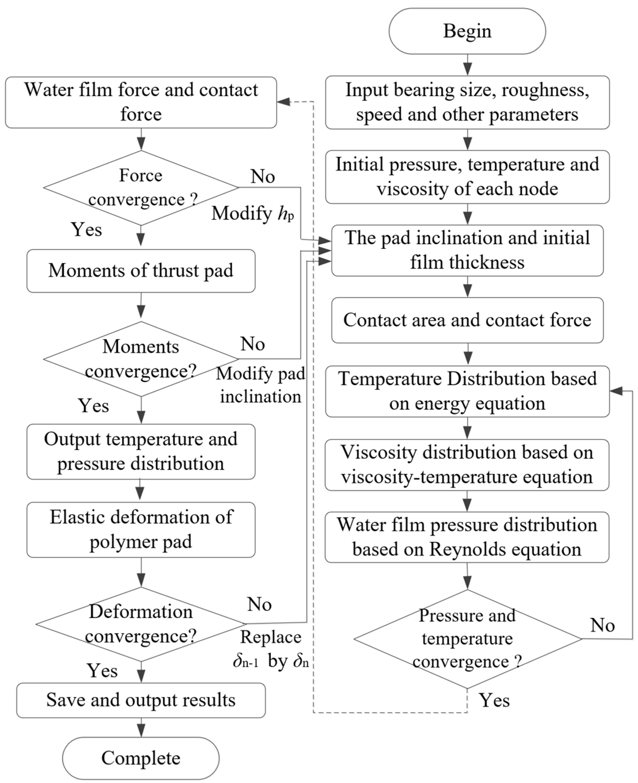
The condition for the pad supported by the elastic cushion to reach the force balance is that the hydrodynamic pressure of the water film and the contact force of the micro-convex body are equal to the external axial load and the moment balance of the tilting thrust pad in the circumferential and radial directions. The viscosity temperature equation and energy equation are also the same as those in this literature. The calculation results will be output when the force, temperature, film thickness and other conditions of the pad meet all the convergence conditions.
A flow chart of the ML calculation model is shown in
Figure 6. The calculated results are automatically renewed according to the simulation code and are considered acceptable when the convergence criteria are satisfied.
3. Results
Herein, the relationship between the thrust collar speed and the water film thickness is obtained using the established mixed lubrication deterministic model. The performance of mixed lubrication, THD lubrication, and TEHD lubrication are compared, and the calculated water film distribution by the mixed lubrication model is also compared with the measured results. According to the distribution of surface roughness measured for many times, the root mean square of surface roughness Sq is no more than 2 μm, and the autocorrelation length ratio λ is pretty close to 1. Therefore, the Sq and λ in all cases in this paper are within this range. Moreover, the thrust pad is divided into 129 and 129 grid elements, which is equivalent to a total of 16,900 micro-asperities or micro-pits on the pad surface. Compared with the soft polymer material, the surface of the thrust collar can be considered rigid and has lower surface roughness, so the thrust collar is assumed to be a smooth rigid plane.
3.1. Variation of Film Thickness and Pressure during Start-up and Acceleration
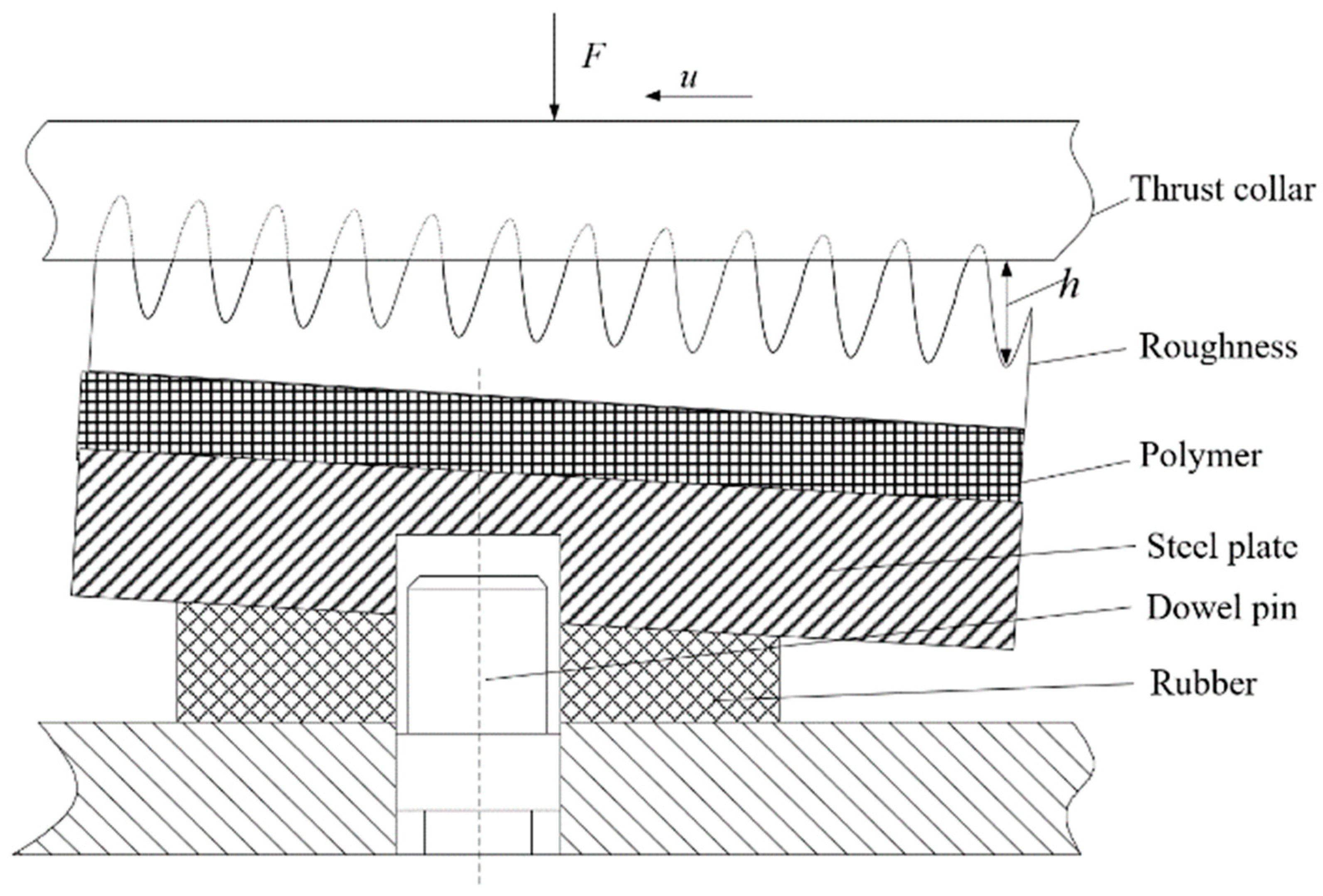
When the bearing is loaded and maintains a static state, the thrust collar and the pad will not fully contact when considering the roughness between the interface, and the axial load is carried by some micro-convex bodies. Since the rubber pad is offset from the pad steel plate base, the thrust pad is inclined under the force of the thrust collar, as shown in
Figure 7. The surface roughness is composed of micro-convex and micro-concave bodies, which can store lubricating cooling water. Taking the distance between the thrust collar and the bottom of the concave as the water film thickness h, the tilting state of the pad can make the water film thickness increase gradually from the outlet side to the inlet side. Therefore, it can be considered that a convergence gap has been formed between the pads and the thrust collar in the static state, which is conducive to the establishment of the lubricating water film during the startup process.
When the bearing accelerates from the static state to the rated speed, with the gradual establishment of the water film, the distance between the thrust collar and the pad increases gradually, the contact pressure of the micro-convex is replaced by the water film pressure and the contact area decreases. In order to observe the changes of the pressure and film thickness at each node of the pad surface with the rotational speed, the randomly distributed roughness of
Sq = 1 μm and
is generated by using the roughness model. In the case of a specific pressure of 0.5 MPa, the calculation results of film thickness and pressure distribution on the pad surface at 50, 300 and 500 r·min
−1 are shown in
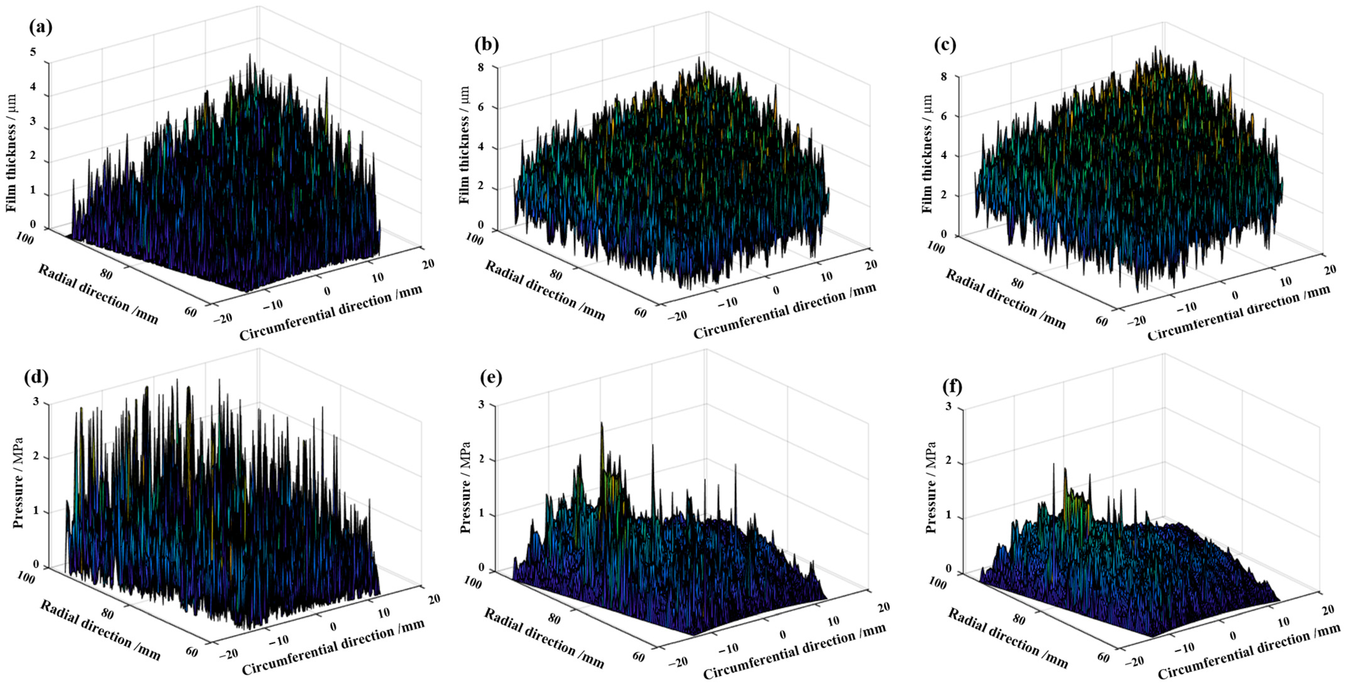
Figure 8, where
Figure 8a–c present the variation law of film thickness distribution. It can be observed that at a low speed of 50 r·min
−1, almost all the outlet sides of the thrust pad are in contact with the micro-convex body, and the film thickness is 0. With the increase in the rotational speed, the film thickness in the outlet area increases correspondingly.
Figure 8d–f show the change rule of pressure distribution, including contact pressure and water film pressure. As shown in
Figure 8d, many pressure peaks can be observed at the outlet side of the pad at 50 r·min
−1, indicating the existence of local contact in this area. The number and amplitude of pressure peaks decrease with the increase in the rotating speed. At 500 r·min
−1, only a few nodes have micro-convex contact, suggesting the improvement of the lubrication condition with the increase in speed.
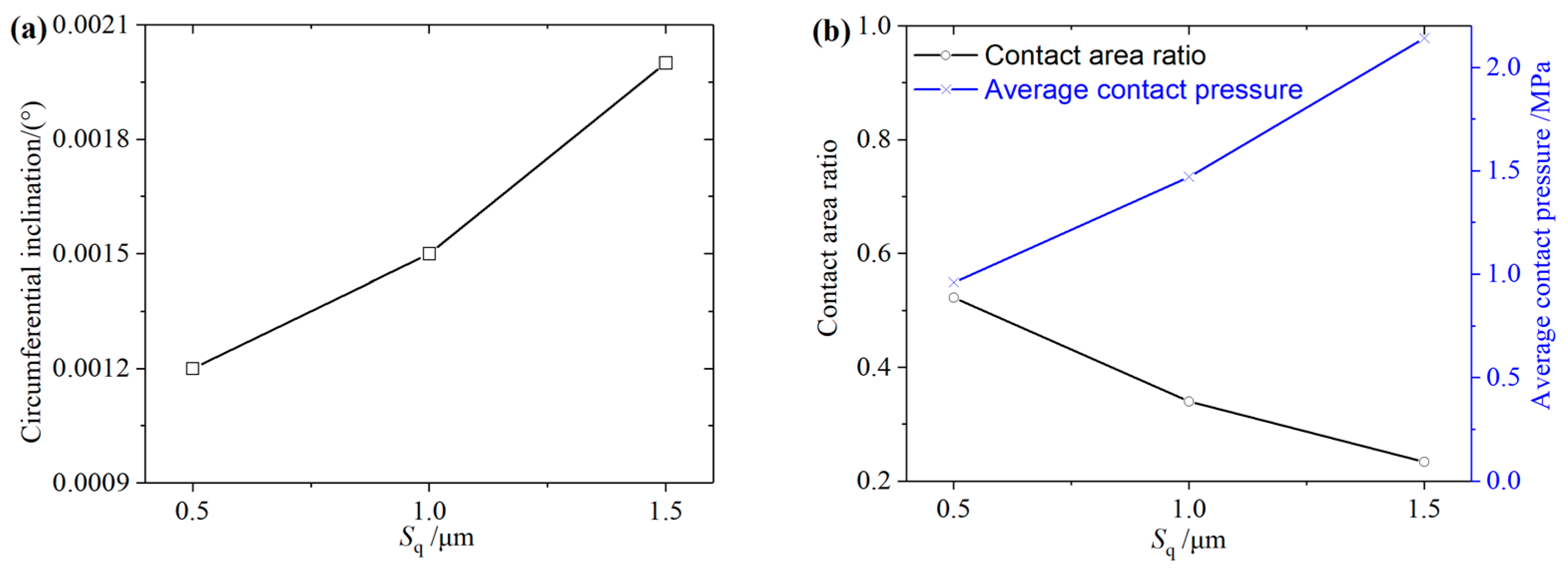
The change rule of thrust pad inclination, contact area ratio and average contact pressure with
Sq is calculated when the bearing is at standstill condition under 0.5 MPa specific pressure, as shown in
Figure 9. Contact area ratio refers to the ratio of the total contact area A of the micro-asperities to the surface area of the thrust pad. It can be seen from
Figure 9a that the circumferential inclination of the pad increases with the increase in
Sq. As shown in
Figure 9b, the contact area ratio decreases with the increase in
Sq, but the change trend of the average contact pressure is the opposite. It shows that with the increase in the roughness height, the inclination angle of the pad increases, and the number of micro-asperities contacting the thrust collar decreases, while the local contact pressure increases. The increase in local contact pressure is generally accompanied by the increase in the risk of wear during startup; that is, the rougher the surface is, the easier it is to be worn during contact friction.
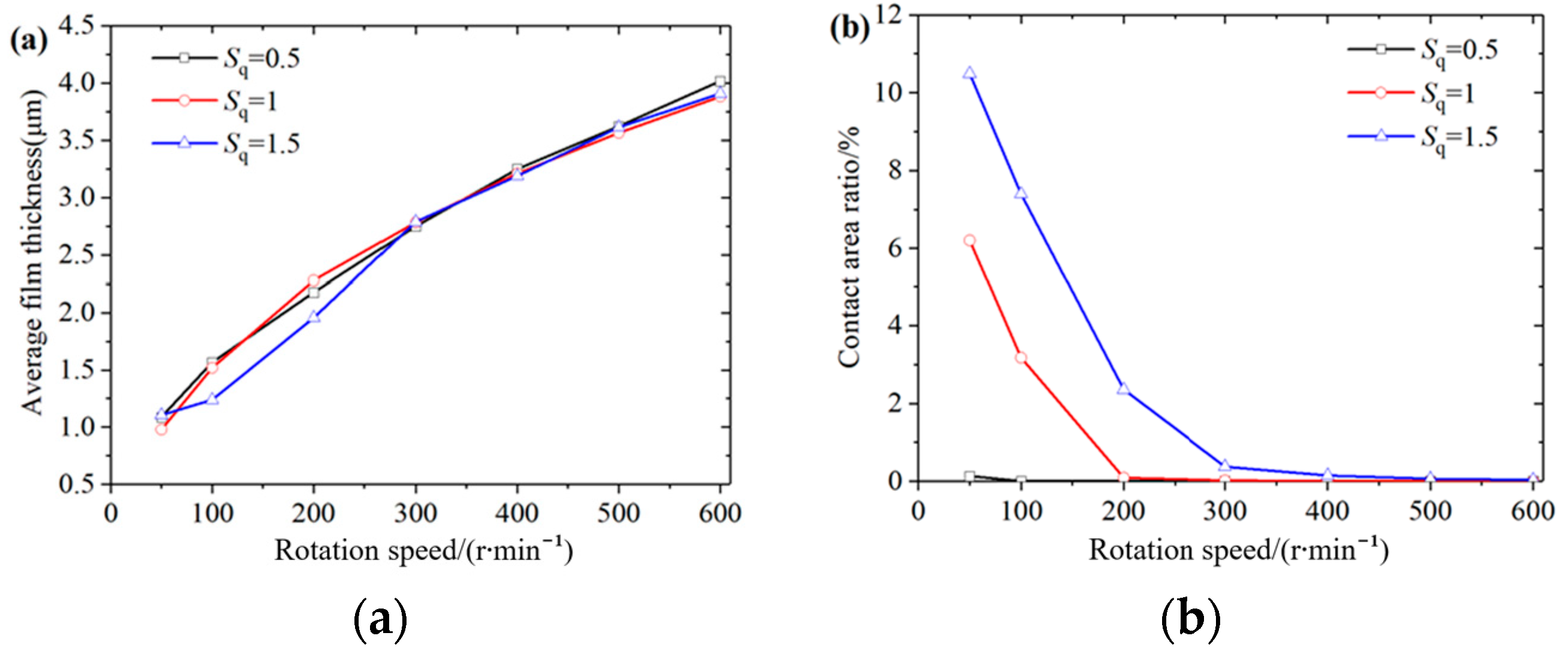
Considering the random surface roughness generated by the mathematical model, five groups of pad surface roughness distributions are randomly generated for
Sq = 0.5, 1, 1.5 μm and
, respectively, to calculate the influence of roughness on the mixed lubrication performance more accurately at the acceleration period, and the lubrication performance of pads with each roughness is calculated and averaged. When the specific pressure is 0.5 MPa, the variations of the average film thickness hm and the contact area ratio of the bearing for the thrust collar accelerating from 50 r·min
−1 to 600 r·min
−1 are shown in
Figure 10.
Figure 10a shows the variation of average film thickness with the increase in roughness. At a low speed of 50 r·min
−1, the average film thickness of the tile with different roughness is relatively close, all about 1 μm, which may be attributed to two reasons: (1) The greater the roughness is, the greater the height of the micro-asperities will be, and the film thickness of the corresponding position will decrease. However, at the same time, the depth of the micro-pit also becomes larger. Hence, the average film thickness is related to the depth at which the vertex of the pad is “pressed” into the thrust collar. The smaller the
Sq is, the smaller the depth at which the vertex of the tile is “pressed” into the thrust collar, the larger the average film thickness should be; (2) The circumferential inclination angle of the pad with large roughness in the low-speed stage will increase the average value of the water film thickness at the entrance, thereby increasing the average film thickness of the entire pad. These two reasons influence each other, so that the average film thickness of the pad at different roughness is close. With the increase in the rotational speed, the average film thickness increases, but that corresponding to pads with different roughness is not much different. It is explained that when the roughness
Sq value changes, the average film thickness
hm is no longer suitable to be used for judging the lubrication performance.
Figure 10b describes the change rule of contact area ratio with roughness and speed. At a speed of 50 r·min
−1, the percentage of the asperities contact area ratio of the thrust pad surface is 0.14%, 6.3% and 10.6%, respectively, while at 200 r·min
−1, there is no contact between the thrust pad and the thrust collar with
Sq = 0.5 μm. This indicates that the bearing is under hydrodynamic lubrication. However, the contact area ratio of the pad with
Sq = 1 μm and 1.5 μm is 0.09% and 2.4%, respectively. Until 600 r·min
−1, the latter two still have a small amount of asperities contact, suggesting a great influence of the roughness height on the contact area ratio and the lubrication state. The higher the roughness is, the higher the rotational speed required for the bearing to achieve full hydrodynamic lubrication becomes.
3.2. Comparison of Lubrication Performance of Different Models
The calculation results based on three different lubrication models (the mixed lubrication model, the THD model and the TEHD model) under rated working conditions are hereby compared. The roughness and working conditions include: root mean square of surface roughness, Sq = 0.5 μm and autocorrelation length ratio , as well as a specific pressure of 0.5 MPa and a speed of 600 r·min−1. The THD model can be evolved from the TEHD model. When the materials of two friction interfaces are set as rigid, the TEHD model becomes the THD.
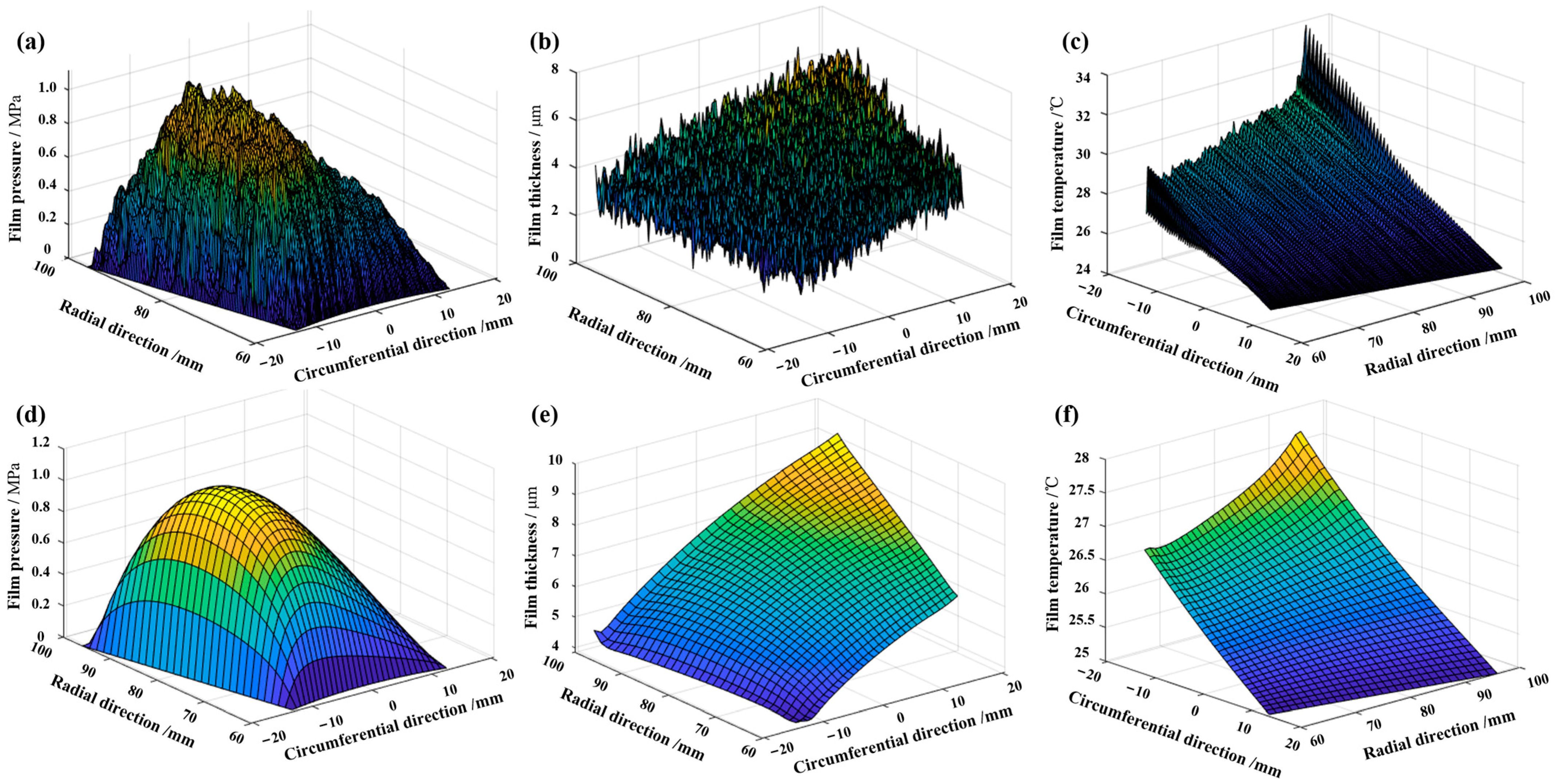
Figure 11 depicts a comparison of water film pressure, thickness and temperature distribution calculated by using the mixed lubrication model and the TEHD model. It demonstrates that the surface roughness makes the distribution of water film pressure, thickness and temperature “rough”.
Figure 11b,e demonstrate that the roughness decreases the film thickness and the circumferential tilting angle of the pad.
Figure 11c,f show that the water film temperature distribution is no longer a smooth surface due to the influence of roughness, but its change law is still increasing along the circumference. At the inner and outer edges near the outlet side, the temperature increases rapidly, and the fluctuation amplitude increases as well.
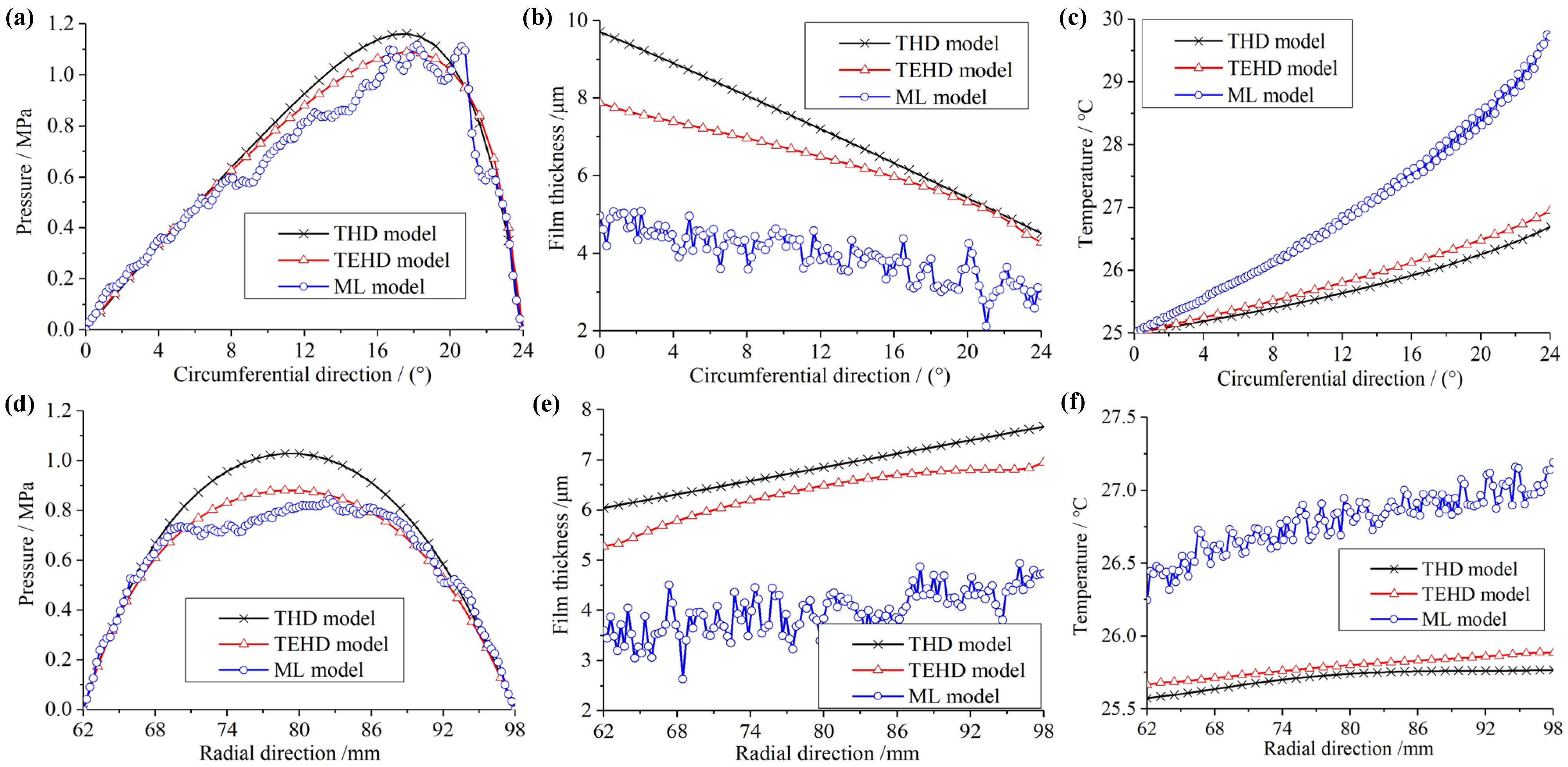
Five groups of randomly distributed roughness with
Sq = 0.5 μm were generated using the mathematical surface roughness model, representing the random distribution of the thrust pad surface roughness. The mixed lubrication model was used to calculate the lubrication performance of bearings with these five groups of roughness. Meanwhile, the water film pressure, thickness and temperature parameters on the average radius and the radial symmetry axis were extracted from the five results and averaged, and then compared with those of the THD model and the TEHD model, as shown in
Figure 12.
In terms of water film pressure distribution, it can be seen from
Figure 12a,d that the change trends of the three are generally consistent. The pressure in the pad middle area on the radial symmetric axis calculated by the THD and TEHD lubrication models is higher than that calculated by the ML model, and the latter generates a pressure distribution greater than the former in the pad edge area to balance the axial load.
Figure 12b,e show the comparison of the water film thickness calculated by the three lubrication models. The water film thickness decreases significantly after using the ML model. Taking the average film thickness as the comparison reference, the values calculated by the THD and TEHD models are 7.24 μm and 6.25 μm, respectively. However, the thickness calculated by the mixed lubrication model is only 3.96 μm. The result calculated by the ML model is 54.7% and 63.4% of the TEHD and the THD model, respectively. If the min film thickness at the pad outlet vertice is used as the comparison reference, the values calculated by the THD model and TEHD model are 4.25 μm and 3.86 μm, respectively. While the result calculated by the ML model is only 2.69 μm, which is 63.3% and 69.7% of the value calculated by the TEHD and the THD model, respectively.
Figure 12c,f present the comparison of water film temperature calculated by the three lubrication models. The calculation results of the ML model are significantly higher than those of the THD and TEHD models, which is mainly attributed to the large decrease in water film thickness. When the water film thickness decreases, both the friction shear force and the friction heat generation increase.
From the comparison of calculation results of the three lubrication models in
Figure 12, the pressure, thickness and temperature calculated by the TEHD model are distributed between the results calculated by the THD model and the mixed lubrication model, perfectly revealing the influence of deformation and surface roughness of the “soft” material on the lubrication performance of the RWTB.
3.3. Comparison between Measurement Results and Calculation Results of Mixed Lubrication Model
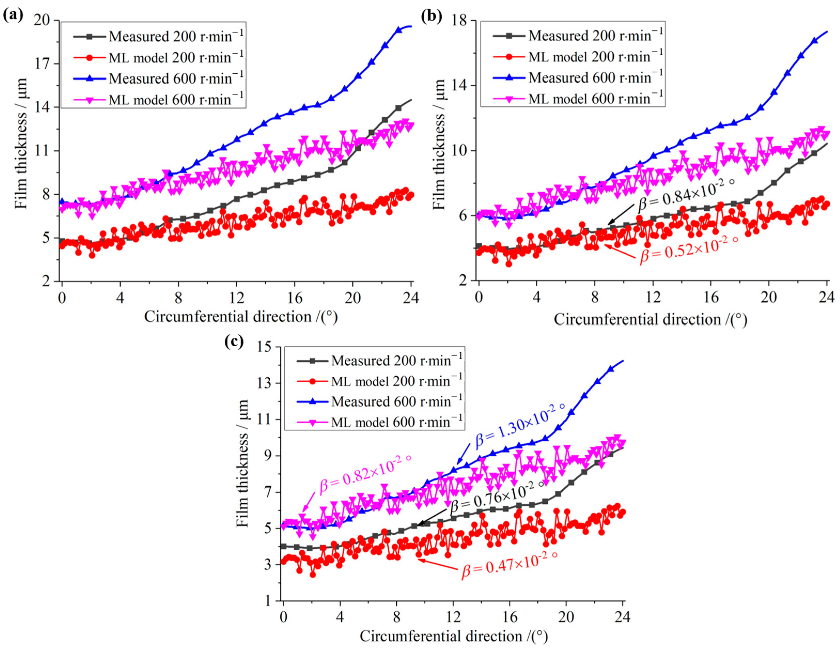
An optical technique is used to measure the water film thickness of RWTB, as described in detail in Reference [
27]. Film thickness distributions are obtained at several specific speeds and loads. The comparison of water film thickness distribution on the
y-axis under specific pressure loads of 0.15, 0.20 and 0.25 MPa and speeds of 200 and 600 r∙min
−1 is shown in
Figure 13, where it can be observed that the film thickness at the outlet side of the pad is in good agreement under different working conditions. However, the discrepancy increases gradually from the outlet side to the inlet side. Taking the case where the specific pressure equals 0.2 MPa and a rotational speed of 200 r·min
−1 as an example, both the calculated and measured minimum film thickness on the
y-axis is 4.0 and 3.7 μm, respectively, with a discrepancy of about 7.5%. However, the calculated circumferential inclination angle (β) of the pad is small, which is 0.0052° and 0.0084°, respectively, suggesting a large film thickness discrepancy near the inlet side. At the circumferential 19° position, the film thickness of the two is 5.9 and 7.1 μm, with a discrepancy of 17%. The comparison between the calculated results of the three models and the measured results shows that the mixed lubrication model can more accurately evaluate the lubrication performance of the RWTB.


