Theoretical Study on the Dynamic Characteristics of Marine Stern Bearing Considering Cavitation and Bending Deformation Effects of the Shaft

Abstract

When the ship runs, owing to the superposition of the gravity of the shaft and resistance of water, with the increment in rotational speeds, the shaft will produce different degrees of bending deformation, which immensely reduces the power transmission efficiency. Based on the aforementioned problem, the present study focuses on the influences of bending deformation of the shaft with a cavitation effect on the dynamic characteristics of the stern bearing. The mixed lubrication model with bending deformation and cavitation effect is established. At present, the deflection curve equation is employed, the finite perturbation method is applied to calculate the dynamic coefficient, and the cavitation pressure is determined by the numerical method. According to the analysis, the variation laws of equivalent stiffness and natural frequency are exhibited. It is shown that the equivalent stiffness is more affected by the speeds, especially at low speeds; There is a critical speed between 130 rpm and 150 rpm, which makes the natural frequency strike the maximum value. Finally, the research results provide a theoretical basis for the ships to avoid large vibration during navigation.

1. Introduction

The lubricants can be employed to form the hydrodynamic, decrease the friction and wear in bearings, intensify load–carry capacity and reduce the mechanical vibration. For the journal bearing, the lubricant forms the hydrodynamic film to support the external loads when the three conditions (the wedge gap, relative velocity and the viscous fluid) are met. In addition, the lubrication mode of journal bearings in ships is mainly water lubrication. Therefore, the present research focuses on water-lubricated bearings.

The studies on water-lubricated bearings have been implemented by plenty of scholars, and the relevant vibration performances and lubrication behaviors are acquired and analyzed. As the crucial part of the submarine or ship, the stiffness and damping properties have a crucial effect on the critical velocity and the stability of ships (as can be seen in Figure 1). For simplifying the analysis on stability, the bearing forces are linearized and adopted to be the linear function for velocity and displacement. According to the method mentioned above, there are eight dynamic coefficients, including four damping coefficients and four stiffness coefficients [1]. For these coefficients, plenty of works are implemented by scholars, and some typical conclusions and results are proposed. Sternlicht [2] expressed the bearing force vector as the linear function of the displacements and static bearing force found the equilibrium position. Sternlicht [2] carried out the relevant investigation. The force vector is adopted as the linear function of static bearing force and displacement to locate the equilibrium point. In his study, by using the Finite Difference Method (FDM), four stiffness coefficients and two direct damping coefficients were given. For the dynamic characteristics, a perturbation solution method of the Reynolds equation is proposed by Lund [3,4]. As noted, the method decreases the demand for numerical differentiation.

The first order perturbation solution is employed in Reinhardt’s study [5]. For the dynamic characteristics of the journal bearing with grooves, two perturbation methods (infinitesimal perturbation method, IFPM and finite perturbation method, FPM) are applied in Someya’s investigation [6]. Nowadays, IFPM and FPM are frequently employed for analyzing dynamic characteristics [7,8,9,10]. Due to the shortcomings of conventional methods in studying the fluid–solid interaction of the bearing–rotor system, Lin [11] explored the two-way fluid–solid interaction and hydrodynamic lubrication performances with thermal effect and cavitation effect by computational fluid dynamics (CFD). In addition, the variation laws of dynamic coefficients under the misalignment are also explored [12,13,14,15]. The influences of the misalignment on the dynamic characteristics are shown in the research of Bou-Said [16] and San Andres [17]. In Qiu’s research [18], for the static loads, the static and dynamic characteristics (attitude angle, friction force, moment and dynamic coefficients, etc) are analyzed under different misalignments and eccentricity ratios. For the water-lubricated bearings, the static and dynamic characteristics are investigated by Feng [19] and Hanawa [20]. Thermohydrodynamic, turbulent and inclined effects were taken into account in the revised models. Lin [21] and Liang [22] performed research on the dynamic characteristics of water-lubricated bearings with grooves. Cavitation effects were considered for the lubrication model. Research indicated that cavitation had more effects on the stiffness coefficients than the damping coefficients.

Therefore, based on the mentioned above, the studies on the influences of cavitation effect on journal bearing are abundant. However, for the coupling effect of bending deformation and cavitation effect, there is little literature. Consequently, a related investigation is carried out.

When the shaft runs, the journal deformation is caused by the force acting on it. Subsequently, the deformation has significant effects on the pressure profile and the asperity contact force under a mixed lubrication condition. Meanwhile, the hydrodynamic force and the asperity contact force jointly act on the journal and affect the deformation. In addition, when the bearing width is large, the deformation of the shaft cannot only be described by two misalignment angles (β and γ) [14]. With the exception of the influences of pressure, asperity contact force and bending deformation of the shaft, the shaft also supports the concentrated load from the propeller. In this study, the interaction between lubrication properties and deformation journals has been taken into consideration. The study applies the deflection curve equation to express the bending deformation. The finite perturbation method is selected to simplify the mathematical model. Moreover, the problem of the mixed lubrication with JFO cavitation condition on a marine stern tube bearing is presented. The effects of bending deformation of the propeller, as well as lubrication boundary conditions, on the dynamic coefficients, are analyzed.

2. Theory Modelling

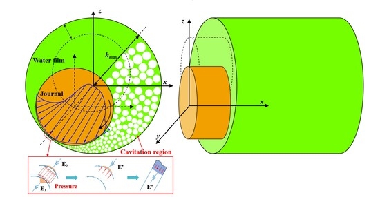
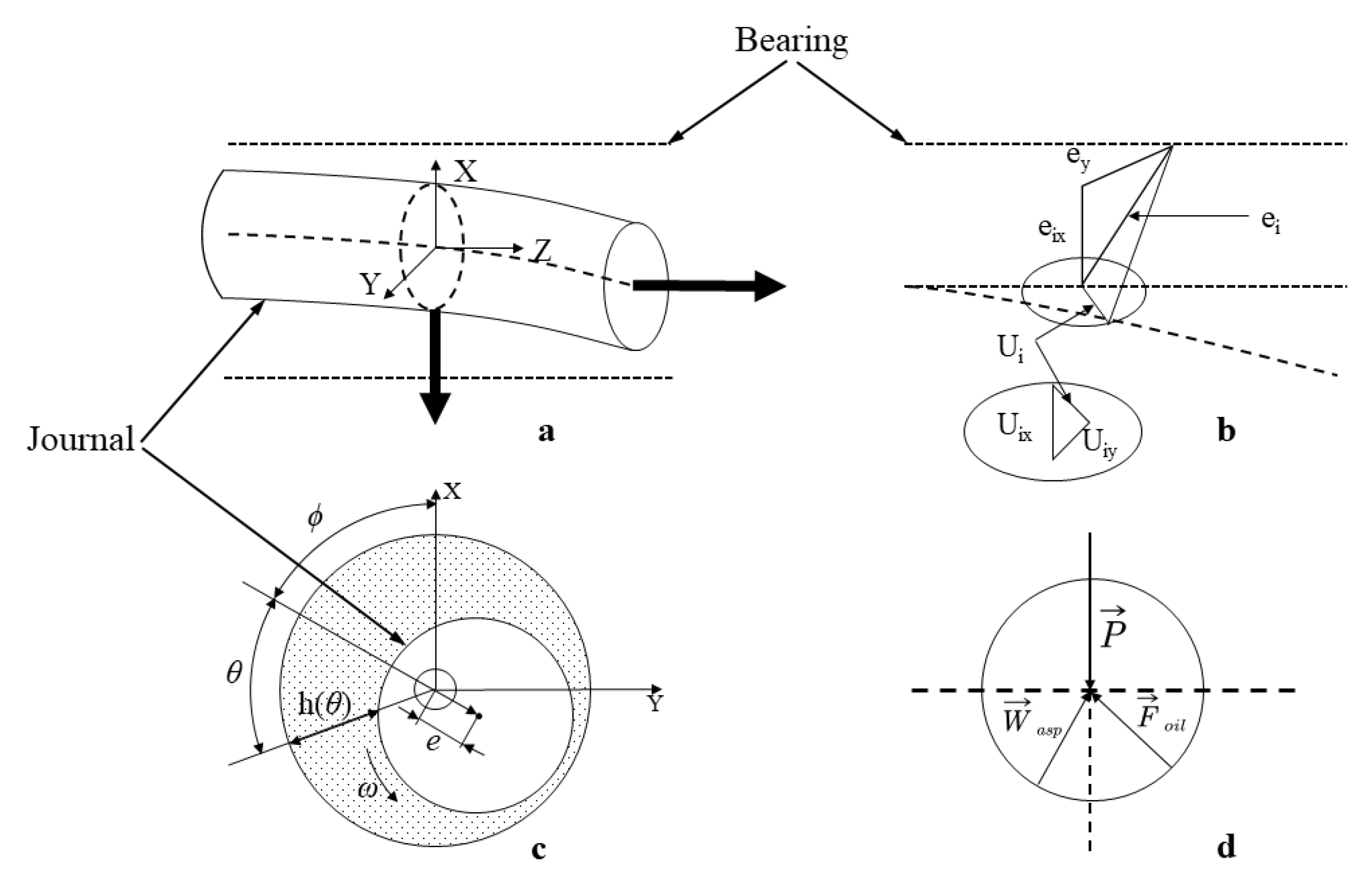
2.1. Characteristics of Journal Bearing

A typical lubricated cylindrical journal bearing is displayed in Figure 2. According to the references describing the lubrication properties of journal bearing, it is obvious that the hydrodynamic pressure rises to a peak in the converging film region and drops to the atmospheric pressure level at both ends. However, in some special areas where the film thickness partially raises, the pressure descends to an ambient level on the contrary. The water evaporation is caused by the released gas from the lubricant or the ambient pressure below the vapor pressure. The rupture of water film is a crucial feature for the stability of the bearing, and the phenomenon is called lubricant cavitation. The research [23,24] explored the effects of cavitation on stability and bearing performances.

Because cavitation collapse can cause severe surface material damage, the cavitation phenomenon should be tried as a very important study direction. Moreover, the beginning and degree can change the load-carrying capacity. The cavitation has a significant effect on the stability of the bearing-rotor system and the maximum amplitude of vibration and whirl [25].

In common, the main function of hydrodynamic pressure is that it provides the wedge space and squeeze effect. The JFO model applies to the dynamic loads that the surface is at the squeeze motion of film [26]. The time variation parameters of rupture film are included in the continuity equation but the bubble dynamics are not considered. With the fluctuation of surface squeeze velocity, the shape of cavitation changes.

In the JFO model, however, since the cavitation zone is unknown during the operating condition, is hard to solve the Reynolds equation numerically. A current cavitation algorithm is developed by Elrod [27,28]. In his research, JFO model has included the Reynolds equation. For the model, the fluid bulk modulus (κ) is used to relate lubricant pressure and density. The boundary conditions at the cavitation area are automatically met by the switch function. Moreover, under cavitation area and integrity film, the feature of continuity equation is transformed from ellipse to parabola by the switch function. Then a variable (θ in [29,30]) is introduced to indicate different lubrication regions (full film region and cavitation).

For the compressible liquid, the relationship between density and pressure is shown as follows:

$$\kappa =\rho \frac{\partial P}{\partial \rho }$$

(1)

And define the density ratio as:

$$\alpha =\frac{\rho }{{\rho }_{cav}}$$

(2)

Then Equation (2) can be rewritten as:

$$g\kappa =\frac{\rho }{{\rho }_{cav}}\frac{\partial P}{\partial \left(\rho /{\rho }_{cav}\right)}=\alpha \frac{\partial P}{\partial \alpha }$$

(3)

where g is defined as a switch function in [29,30] and values of g in different zones are described as:

$$g=\left\{\begin{array}{l}1 whole film zone\\ 0 cavitation zone\end{array}\right.$$

For Equation (3), the direct integration is implemented, and then the following equation can be obtained:

$$P=P_{cav}+g\kappa \ln \left(\alpha \right)$$

(4)

It should be indicated that for the part of whole film, $g=1$ and $P>P_{cav}$, since $\alpha =\frac{\rho }{{\rho }_{cav}}>1$; and for cavitation area $P=P_{cav}$ because of $g=0$. As noted, pressure gradient is a crucial factor for the thin film flow. Consequently, for $P_1$ and $P_2$, they are larger than $P_{cav}$,

$$P_1-P_2=\kappa \left[\ln \left({\alpha }_1\right)-\ln \left({\alpha }_2\right)\right]\cong \kappa \left({\alpha }_1-{\alpha }_2\right)$$

(5)

Owing to the large magnitude of $\kappa$, the slight difference in density ratio can result in a tremendous difference in pressure. In addition, for the numerical model, there are a few difficulties because of the different considerations. For the variable $\alpha$, under the whole film area and cavitation area, the explanation is different [31]. In cavitation area, due to the vapor material within the cavity, the density of water is even (${\rho }_{cav}$) and the wedge gap is not stuffed. Therefore, $\alpha$ is recognized as the small film content and the void fraction can be expressed by the ($1-\alpha$).

Based on the mass flow conversation of thin film:

$$\frac{\partial \left(\rho h\right)}{\partial t}+\frac{\partial \left(M_x\right)}{\partial x}+\frac{\partial \left(M_z\right)}{\partial z}=0$$

(6)

Under the full film area, for the mass flow rate of fluid, it can be shown as:

$$M_x=-\frac{\rho h^3}{12\mu }\frac{\partial P}{\partial x}+\frac{\rho hU}{2}; M_z=-\frac{\rho h^3}{12\mu }\frac{\partial P}{\partial z}$$

(7)

However, for the cavitation position, $\frac{\partial P}{\partial x}=\frac{\partial P}{\partial z}=0$, the mass flow rate is:

$$M_x=\alpha {\rho }_{cav}h\frac{\Omega R}{2}; M_z=0$$

(8)

Due to $\partial P=\frac{\kappa }{\rho }\partial \rho =g\frac{\kappa }{\alpha }\partial \alpha$, Equation (7) can be derived as:

$$M_x=-\frac{{\rho }_{cav}{h}^3}{12\mu }g\kappa \frac{\partial \alpha }{\partial x}+\alpha \frac{{\rho }_{cav}hU}{2}; M_z=-\frac{{\rho }_{cav}{h}^3}{12\mu }g\kappa \frac{\partial \alpha }{\partial z}$$

(9)

As noted, under the full film area ($g=1$ and $\alpha =\rho /{\rho }_{cav}$) and cavitation position, $g=0$ with $\alpha$ is recognized as the small film content.

Equation (6) can be solved by the global mass conservation as:

$$\frac{\partial }{\partial x}\left(\frac{{\rho }_{cav}{h}^3}{12\mu }g\kappa \frac{\partial \alpha }{\partial x}\right)+\frac{\partial }{\partial z}\left(\frac{{\rho }_{cav}{h}^3}{12\mu }g\kappa \frac{\partial \alpha }{\partial z}\right)={\rho }_{cav}\frac{\partial \left(\alpha h\right)}{\partial t}+{\rho }_{cav}\frac{U}{2}\frac{\partial \left(\alpha h\right)}{\partial x}$$

(10)

And in the cavitation zone, Equation (10) can be reduced to:

$${\rho }_{cav}\frac{\partial \left(\alpha h\right)}{\partial t}+{\rho }_{cav}\frac{U}{2}\frac{\partial \left(\alpha h\right)}{\partial x}=0$$

(11)

This establishes a dynamic flow balance in the cavitation area. The mixed success is available in the present research by the common cavitation algorithm. However, compared with the rough technology, the common cavitation algorithm is obsolete.

2.2. Bearing Forces

There is a crucial relationship between rotational speed and journal position. The relation equation can be expressed by the bearing force.

$$F_x=F_x\left(x,y,\dot{x},\dot{y}\right), F_y=F_y\left(x,y,\dot{x},\dot{y}\right)$$

(12)

By numerical procedure, as long as the film pressure is determined, the pressure in a horizontal and vertical direction is integrated to acquire the bearing force:

$$\left[\begin{array}{l}{F}_x\\ F_y\end{array}\right]=-{\displaystyle {\int }_{{\varphi }_0}^{{\varphi }_2}{\displaystyle {\int }_0^L\left[\begin{array}{l}\sin \varphi \\ \cos \varphi \end{array}\right]}}\left(Rd\varphi \right)dz=-C_g{\displaystyle {\int }_{{\varphi }_0}^{{\varphi }_2}{\displaystyle {\int }_0^{L/R}\left[\begin{array}{l}\sin \varphi \\ \cos \varphi \end{array}\right]}}d\varphi dz$$

(13)

2.3. Attitude Angle

The angle between the load direction and the central line that connects the bearing and journal is the attitude angle. Under stable condition, the bearing forces are employed to balance the external loads. According to the external load $W$, the bearing force vector is shown by the load-carrying capacity vector:

$$\overrightarrow{W}={\overrightarrow{F}}_x+{\overrightarrow{F}}_y$$

(14)

If the $W$ acts on the vertical direction (such as the weight of the screw propeller in this study), the horizontal force is ${\overrightarrow{F}}_x=0$. Therefore:

$${\tan }^{-1}\frac{F_x}{F_y}=0$$

(15)

The error function is defined as:

$$d{\varphi }_0^k={\tan }^{-1}\frac{F_x^k}{F_{{}_y}^k}$$

(16)

If $d{\varphi }_0^k=0$, the condition of Equation (15) is met automatically. In order to calculate $d{\varphi }_0^k=0$, the Newton-Raphson iteration method is adopted:

$${\varphi }_0^{k+1}={\varphi }_0^k-\frac{d{\varphi }_0^k}{\left(d{\varphi }_0^k-d{\varphi }_0^{k-1}\right)/\left({\varphi }_0^k-{\varphi }_0^{k-1}\right)}$$

(17)

The ${\varphi }_0^k$ is considered the attitude angle ${\varphi }_0$. In the numerical procedure, if

$$d{\varphi }_0^k=\left|{\tan }^{-1}\frac{F_x^k}{F_{{}_y}^k}\right|\le {\delta }_{\varphi }$$

(18)

Once ${\varphi }_0$ is converged, $P_{i,j}$ and water film boundaries can be determined.

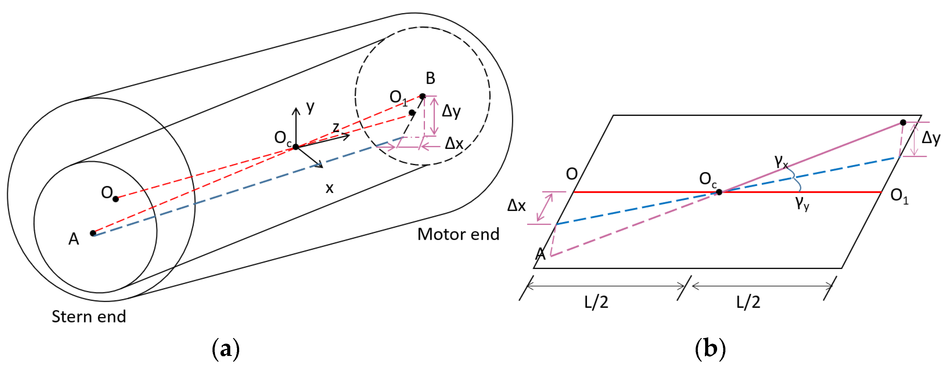
2.4. Film Thickness Considering Bending Deformation of Journal

When the relative rotating speed exists between the journal and bearing, the eccentricity amount adjusts automatically until the film pressures calculated by the average Reynolds equation and the asperities contact pressures calculated by the contact model balance the external loads. From the description of lubrication properties, the film pressures and the contact pressures depend on the local film thickness. In addition, the misalignment parameters give the expression of film thickness of misaligned bearing ($\beta$ and $\gamma$) [14], as Equation (19) shows:

$$h_{\theta }=c+e_0\cos \left(\theta -\phi \right)+z\tan \gamma \cos \left(\theta -\beta -\phi \right)$$

(19)

When it comes to the large width of the bearing, the deflect angle in each journal section is different as a result. After considering the bending deformation of the shaft, the film thickness can be briefly expressed as:

$$h_{i\theta }=c+e_i\cos \left(\theta -\varphi \right)$$

(20)

Define $e_i=\sqrt{{\left({\upsilon }_{ix}+e_{ix}\right)}^2+{\left({\upsilon }_{iy}+e_{iy}\right)}^2}$, when the shaft is bending deformation, for the ith section, the eccentricity ratio is $e_i$; $e_{ix}$ and $e_{iy}$. These are the components of the eccentricity ratio without bending in horizontal (x) and vertical (y) directions (as shown in Figure 3). The deformation of this section is ${\upsilon }_i=\sqrt{{\upsilon }_{ix}{}^2+{\upsilon }_{iy}{}^2}$, and in order to determine ${\upsilon }_i$ accurately, the displacement superposition method is applied to calculate the bending deformation in this study (as shown in Figure 4).

2.5. Determining the Bending Deformation of Journal

Obviously, the force that acts on the shaft results in the bending deformation of the shaft. Due to the reaction relationship, the deformation will change the profile of film pressure. If the ratio of film thickness to surface roughness is less than 4 [30], the asperity contact force of the end is seriously affected. In [14], Sun used $\gamma$ to describe the misaligned angle of the shaft in bearing, and it can be expressed as:

$$\gamma =\frac{F_{ex}{l}^2}{16E_{j}I}$$

(21)

However, as per the reason mentioned in Section 2.4, it should be noted that the misaligned angle in each section of the shaft is various in the very wide bearing. During this study, in the axial direction, the whole bearing is divided into 20 sections. For the sake of accurate determination of the bending deformation, the differential equation of the deflection curve (given as following) is used:

$$\frac{d^2\upsilon }{d{x}^2}=\frac{M\left(x\right)}{EI}$$

(22)

When it comes to the loaded stern shaft shown in Figure 3. Under sophisticated load conditions, owing to the small bending deformation of the shaft, the shaft material is recognized as elastic, based on the conclusion of [31]. The displacement superposition method can be applied in this study to solve bending deformation. From superposition theory, in the systems subject to multiple loads, resultant stress or strain is the algebraic sum of its effects when the load is applied alone. Taking a cantilever beam as an example, the solution of this beam under typically single-load conditions is shown in

Table 1. The cases exhibition of in cantilever beam.

Loading Condition	$\mathbf{Deflection} \left(\mathit{\upsilon }\right)$
Concentrated load P at end	$\upsilon =-\frac{P{z}^2}{6EI}\left(3l-z\right)$	(23)
Concentrated load P at point a	$\begin{array}{l}\upsilon =-\frac{P{z}^2}{6EI}\left(3a-z\right)\hspace{1em}0\le z\le a\\ \upsilon =-\frac{P{a}^2}{6EI}\left(3z-a\right)\hspace{1em}a\le z\le l\end{array}$	(24)

. The sum of these solutions can be also employed to express the deformation caused by external loads and asperity contact force.

As described previously, in the axis direction, the journal is divided into 20 rigid nodes, and in z direction, for the ith node, the coordinate is $Z_i$. For the bending deformation of the shaft, the ith section is ${\upsilon }_{ix}$ and ${\upsilon }_{iy}$. For the hydrodynamic force and asperity contact force, at the ith section center, they are expressed as $F_{ix}$ and $F_{iy}$, $W_{ix}$ and $W_{iy}$. As noted, the subscript of x indicates the x direction, for the subscript of y, the meaning is identical. In addition, the resultant forces of both are $F_i$ and $W_{asp}$, respectively.

According to Equations (15) and (16), for all nodes of the journal, the bending deformation is displayed as:

when $z=z_i (1, k)$,

$$\begin{array}{l}{\upsilon }_{zx}=-\frac{P{z}_k{}^2}{6EI}\left(3l-z_k\right)-{\displaystyle \sum _{i=1}^k\frac{\left(F_{ix}+W_{ix}\right)z_i{}^2}{6EI}\left(3z_k-z_i\right)}-{\displaystyle \sum _{i=k+1}^n\frac{\left(F_{ix}+W_{ix}\right)z_k{}^2}{6EI}\left(3z_i-z_k\right)}\\ {\upsilon }_{zy}=-{\displaystyle \sum _{i=1}^3\frac{\left(F_{iy}+W_{iy}\right)z_i{}^2}{6EI}\left(3z_k-z_i\right)}-{\displaystyle \sum _{i=4}^n\frac{\left(F_{iy}+W_{iy}\right)z_k{}^2}{6EI}\left(3z_i-z_k\right)}\end{array}$$

(25)

when $z=z_n$,

$$\begin{array}{l}{\upsilon }_{zx}=-\frac{P{z}_n{}^2}{6EI}\left(3l-z_n\right)-{\displaystyle \sum _{i=1}^n\frac{\left(F_{ix}+W_{ix}\right)z_i{}^2}{6EI}\left(3z_n-z_i\right)}\\ {\upsilon }_{zy}=-{\displaystyle \sum _{i=1}^n\frac{\left(F_{iy}+W_{iy}\right)z_i{}^2}{6EI}\left(3z_n-z_i\right)}\end{array}$$

(26)

According to the above expressions, the bending deformation at mixture load conditions, including the concentrated loads of the propeller, the hydrodynamic pressure and asperity pressures, can be determined accurately.

2.6. The Deformation of Bearing

As an external load is applied to a journal bearing, the bending deformation of the journal has happened, and as Figure 5 shows, the water film thickness is reduced at the sections close to the bearing end; as a result, the film pressure will increase rapidly at those sections. In this situation, in order to analyze the consequences of the pressure distribution and wear phenomena better, the method that the elastic deformation of bearing is included in the elastohydrodynamic model is crucial. At present, the elastic deformation is incorporated into the lubrication characteristics of dynamic bearing that analyzes the various external loads. By calculating the deformation of bearing $\Delta H$ in different conditions and adding it to the film thickness value (as shown in Equation (20)), the influences of elastic deformation on lubrication performances are explored.

In this study, the equivalent model is employed to describe the deformation. From Figure 6, the whole elastic deformation of journal and bearing is expressed by $\Delta H$, and $E_1$, $E_2$ is Young’s modulus of journal and bearing, respectively. The composite of Young’s modulus of bearing and journal is $E^{\prime }$. The deformation corresponds to that of the bearing surface just with composite Young’s modulus. According to the equivalent model, the changing length of the object just with Young’s modulus $E^{\prime }$ and initial length $L$ can be expressed by $\Delta H$. According to the above analysis, the expression [32] is obtained as:

$$P\cong E\prime \epsilon \cong E\prime \frac{\Delta H}{L}$$

(27)

The normal pressure acting on the journal can be acquired by:

$$\Delta H\cong \frac{L}{E\prime }P$$

(28)

2.7. The Pressure in Cavitation Zone

To determine the pressure in the cavitation zone, the equations listed in reference [33] are used in this study, which is given as:

$$P_{cav}=P_{ml}$$

(29)

$$P_{ml}={\rho }_v{C}_v{}^2-N\log \left(\frac{{\rho }_v{}^2{C}_v{}^2}{{\rho }_l{}^2{C}_l{}^2}\right)$$

(30)

$$N=\frac{{\rho }_v{C}_v{}^2{\rho }_l{C}_l{}^2\left({\rho }_v-{\rho }_l\right)}{{\rho }_v{}^2{C}_v{}^2-{\rho }_l{}^2{C}_l{}^2}$$

(31)

As it is summarized in reference [33], Equation (29) could give a better correlation in the transition zone. Based on those equations, the $P_{cav}$ can be quickly determined by ${\rho }_v$, ${\rho }_l$, $C_v$, $C_l$. Define:

$$r_p=\frac{{\rho }_v}{\rho l}$$

(32)

2.8. Calculation of the Dynamic Coefficients

Based on Equation (12), the bearing forces are derived by:

$$F_x=k_{xx}x+k_{xy}y+b_{xx}\dot{x}+b_{xy}\dot{y}$$

(33)

$$F_y=k_{yx}x+k_{yy}y+b_{yx}\dot{x}+b_{yy}\dot{y}$$

(34)

And the eight coefficients are defined as:

$$k_{xx}=\frac{\partial F_x}{\partial x},k_{xy}=\frac{\partial F_x}{\partial y},k_{yx}=\frac{\partial F_y}{\partial x},k_{yy}=\frac{\partial F_y}{\partial y}$$

(35)

$$b_{xx}=\frac{\partial F_x}{\partial \dot{x}},b_{xy}=\frac{\partial F_x}{\partial \dot{y}},b_{yx}=\frac{\partial F_y}{\partial \dot{x}},b_{yy}=\frac{\partial F_y}{\partial \dot{y}}$$

(36)

These eight coefficients are defined as dynamic coefficients of the journal bearing, as shown in Figure 7. According to those references reviewed previously, there are two theoretical methods (IFPM and FPM) to calculate the dynamic coefficients. FPM is used in this study.

2.9. Finite Perturbation Method (FPM)

FPM perturbs the journal under the equilibrium position by the small $\Delta x$, $\Delta y$, $\Delta \dot{x}$ and $\Delta \dot{y}$, and the force finite difference is employed to describe the force coefficient. For the calculation accuracy, the perturbation is implemented in the positive and negative directions, and the partial differential in both directions is adopted to calculate the partial derivative. At the equilibrium position ($x_o$, $y_o$), the partial derivative $\frac{\partial F_x}{\partial x}$ (force coefficient $k_{xx}$) can be solved by [7]:

$$\begin{array}{cc}\hfill k_{xx}=\frac{\partial F_x}{\partial x}& \approx \frac{1}{2}\left[\frac{F_x\left(x_0 + \Delta x,y_0,{\dot{x}}_0,{\dot{y}}_0\right) - F_x\left(x_0,y_0,{\dot{x}}_0,{\dot{y}}_0\right)}{\Delta x}+\frac{F_x\left(x_0,y_0,{\dot{x}}_0,{\dot{y}}_0\right) - F_x\left(x_0 - \Delta x,y_0,{\dot{x}}_0,{\dot{y}}_0\right)}{\Delta x}\right]\hfill \\ & =\frac{F_x\left(x_0 + \Delta x,y_0,{\dot{x}}_0,{\dot{y}}_0\right) - F_x\left(x_0 - \Delta x,y_0,{\dot{x}}_0,{\dot{y}}_0\right)}{2\Delta x}\hfill \end{array}$$

(37)

At the steady state, ${\dot{x}}_o={\dot{y}}_o=0$; thus:

$$k_{xx}=\frac{F_x\left(x_0+\Delta x,y_0,0,0\right)-F_x\left(x_0-\Delta x,y_0,0,0\right)}{2\Delta x}$$

(38)

Similarly, the other stiffness coefficients can be calculated by:

$$k_{yx}=\frac{\partial F_y}{\partial x}\approx \frac{F_y\left(x_0+\Delta x,y_0,0,0\right)-F_y\left(x_0-\Delta x,y_0,0,0\right)}{2\Delta x}$$

(39)

$$k_{xy}=\frac{\partial F_x}{\partial y}\approx \frac{F_x\left(x_0,y_0+\Delta y,0,0\right)-F_x\left(x_0,y_0-\Delta y,0,0\right)}{2\Delta y}$$

(40)

$$k_{yy}=\frac{\partial F_y}{\partial y}\approx \frac{F_y\left(x_0,y_0+\Delta y,0,0\right)-F_y\left(x_0,y_0-\Delta y,0,0\right)}{2\Delta y}$$

(41)

The damping coefficients are acquired by:

$$b_{xx}=\frac{\partial F_x}{\partial \dot{x}}\approx \frac{F_x\left(x_0,y_0,\Delta \dot{x},0\right)-F_x\left(x_0,y_0,-\Delta \dot{x},0\right)}{2\Delta \dot{x}}$$

(42)

$$b_{yx}=\frac{\partial F_y}{\partial \dot{x}}\approx \frac{F_y\left(x_0,y_0,\Delta \dot{x},0\right)-F_y\left(x_0,y_0,-\Delta \dot{x},0\right)}{2\Delta \dot{x}}$$

(43)

$$b_{xy}=\frac{\partial F_x}{\partial \dot{y}}\approx \frac{F_x\left(x_0,y_0,0,\Delta \dot{y}\right)-F_x\left(x_0,y_0,0,\Delta \dot{y}\right)}{2\Delta \dot{y}}$$

(44)

$$b_{yy}=\frac{\partial F_y}{\partial \dot{y}}\approx \frac{F_y\left(x_0,y_0,0,\Delta \dot{y}\right)-F_y\left(x_0,y_0,0,-\Delta \dot{y}\right)}{2\Delta \dot{y}}$$

(45)

The FPM only needs to solve the bearing forces at eight perturbed positions: ($x_0-\Delta x$, $y_0$, 0, 0), ($x_0+\Delta x$, $y_0$, 0, 0), ($x_0$, $y_0-\Delta y$, 0, 0), ($x_0$, $y_0+\Delta y$, 0, 0), ($x_0$, $y_0$, $-\Delta \dot{x}$, 0), ($x_0$, $y_0$, $\Delta \dot{x}$, 0), ($x_0$, $y_0$, 0, $-\Delta \dot{y}$) and ($x_0$, $y_0$, 0, $\Delta \dot{y}$).

If the perturbation magnitude is large, there are some errors in the linear model. This is because the bearing force is a sophisticated nonlinear function. According to the theory, there is a maximum perturbation amplitude. When the amplitude is less than the maximum value, the calculation accuracy is high and acceptable. Applying FPM, the maximum perturbation amplitude can be determined by a given accuracy.

3. Numerical Procedure

Based on the numerical model developed in this study, the solution procedure is shown in Figure 8. In the dynamic part, a combination of FDM and FPM methods is applied. The equation of film thickness is displayed by the nodal global coordinate of the bearing surface. For the analysis of lubrication performances, the computer program is developed. The flowchart of the numerical procedure can be seen in Figure 8. The calculation procedure is designed as follows:

(1)

Input the parameters of the stern bearing, initial film pressure, asperities contact forces and deformation of bearing. The assumption condition for the shaft center is given, and then the deformation of the shaft under external loads (the concentrated load of the propeller) is calculated;

(2)

Calculating the water film shape according to the current journal position through Equation (20) and adding the value of bearing deformation into $h_{i\theta }$;

(3)

Obtain the hydrodynamic pressure distribution by implementing the universal cavitation algorithm; Calculate the asperities contact forces;

(4)

The trajectory position is acquired by the integral for the balance loads, hydrodynamic pressure and asperity contact force. In addition, the over-relaxation Newton–Raphson method is employed to accelerate convergence;

(5)

For the deformation of the shaft under external loads, film pressure and asperity contact force and bearing deformation, the calculation needs to be resolved until they meet the convergence criterion:

$$\left|\frac{e^{k+1}-e^k}{e^k}\right|\le 0.01 \mathrm{and} \left|\frac{{\varphi }^{k+1}-{\varphi }^k}{{\varphi }^k}\right|\le 0.01$$

(6)

In order to determine the bearing force of each perturbation position, step (2)~(5) is recalculated by perturbing the position and velocity of the journal;

(7)

According to Equations (38)–(45), the dynamic coefficients are acquired.

In the analysis, the prediction is mainly decided by the value of the volume modulus ($\kappa$). For the accurate solution, the algebraic equations are stiff because of the actual value of the bulk modulus of water. One reasonable explanation is that the slight variation of density has a significant effect on the hydrodynamic pressure at the full film area. Therefore, for the numerical model, the round-off errors appear [7]. The artificial low bulk modulus is adopted to avoid the problem of accuracy and convergence. As noted, its magnitude is less than the physical value. The excellent results are given by the stable numerical algorithm. The numerical range is 1/100 to 1/10 of the actual physical value.

4. Results and Discussion

4.1. Validation

To validate the present numerical scheme, a result obtained from the present analysis is compared with the results obtained by the experimental data given by Su [34].

Table 2. Parameters of the water-lubricated bearing.

Item	Value
Radius of Bearing (m)	0.05
Radial Clearance (mm)	0.1455
Ratio of Bearing Length and Bearing Diameter	1.333
Eccentricity ratio	0.61
Angular Velocity (rad/s)	48.1
Lubrication Supply Pressure (Pa)	0
Cavitation Pressure (Pa)	−72,139.79

lists the bearing parameters for the comparison case, and Figure 9 shows the film pressure predicted by the model developed in this study and the experimental results from [34]. As shown in this figure, compared with the results gotten from the Reynolds boundary, the film pressure predicted by the JFO boundary matches the experimental results much better. The pressure is recognized as vapor pressure in the Reynolds boundary condition. In addition, at the position of full film rupture, the circumferential gradient must be equal to zero. From the above analysis, compared with the experiment results, the error is large.

Numerical research on the water-lubricated bearing with cavitation is carried out to explore the influences of propeller deformation on the behaviors of the bearing. For the following situation, the water-lubricated stern bearing (shown in Figure 10) variables used in the computation are listed in

Table 3. The parameters and material properties of the marine stern bearing.

Shaft Segment No.		Middle Shaft		Stern Shaft
		1	2	3	4	5
Length (m)		2.9	3.6	1.55	3.45	2.05
Diameter of shaft (cm)		39	39	49.8	49.8	49.8
Young’s Modulus of shaft(N/m2)		2.1 × 1011
Density of shaft (kg/m3)		7850
Poisson Ratio of shaft		0.3
Bearing material (bearing 1, bearing 2 and bearing 3)		Aluminium alloy PTFE
Radial clearance(m)	Bearing 1	0.6 × 10−3
	Bearing 2	0.6 × 10−3
	Bearing 3	0.4 × 10−3
Roughness of shaft (m)		4.3 × 10−6
Roughness of bearing (m)		4.3 × 10−6
Shaft to Bearing contact friction coefficient		0.1
Kinematic viscosity of lubricant (N·s/cm2)		0.15 × 10−6
Ratio of density rp		2.31 × 10−5
Density of the liquid phase of lubricant (kg/m3)		890
Sound velocity of the sound in the pure vapor (m/s)		343
Sound velocity of the sound in the pure liquid (m/s)		1450

. The weight of the screw propeller is 0.21498 × 10⁶ N. According to the validation case, the JFO boundary condition is much closer to the real condition. Therefore, the following analysis is only based on the JFO boundary condition. Meanwhile, the deformations of the bearing and propeller are taken into consideration. The structure of the propeller is shown in Figure 10. The shaft is divided into two parts by the flange. According to the position of the bearings, the whole shaft can be divided into five segments, as shown in Figure 10. The length of each part is listed in Table 3, together with the bearings’ parameters and material properties.

4.2. The Equivalent Stiffness

The dynamic stability and maximum vibration amplitude of the bearing-rotor system are affected by the cavitation to a large extent, especially for the dynamically loaded bearing. The stability of hydrodynamic bearings is generally addressed since the early design stages of a rotor-bearing system. The water film is recognized as the spring with the equivalent stiffness:

$$K_{ss}=m{\omega }^2$$

(46)

Then from [35],

$$K_{ss}=\frac{k_{xx}{b}_{yy}+k_{yy}{b}_{xx}-k_{xy}{b}_{yx}-k_{yx}{b}_{xy}}{b_{yy}+b_{xx}}$$

(47)

And this equivalent stiffness is important in the stability analysis of hydrodynamic bearings. In stability calculation, if $K_{SS}$ < 0, the system is absolutely unstable.

The absolute smooth surface does not exist. Generally, the surface roughness is identical to, or larger than the film thickness estimated by the smooth surface hydrodynamic lubrication theory. Based on the model developed by Patir and Cheng [36], the empirical pressure flow, shear flow factors and asperity contact factor are used in this study. The correlation between relative velocity and coefficient of friction of bearing-rotor system is constructed by Stribeck under constant load to describe the range of different operating conditions. The reference [37] has indicated the relationship between the asperity contact force and lubrication regime, and the bottom of the Stribeck curve is regarded as the transition point of mixed lubrication and hydrodynamic lubrication. Due to the concentrated load of the propeller, the bending deformation is taking place in the whole operating condition. Simultaneously, the journal deformation is affected by the hydrodynamic pressure and asperity contact force [38,39]. Furthermore, for a large width-bearing like the water-lubricated stern bearing in ships (as shown in Figure 10), in the analysis of the bearing-rotor system, the bending deformation of the shaft cannot be ignored. Figure 11 shows the Stribeck curve and the equivalent stiffness $K_{SS}$ in different speeds of bearing 1. From Figure 11, we can see that under hydrodynamic lubrication, the equivalent stiffness $K_{SS}$ decreases with speeds. As noted, the $K_{SS}$ descends sharply under low speeds. However, with the increase in speeds, the trend is inclined to be stable. One reasonable explanation for it is that in hydrodynamic lubrication and the hydrodynamic film forms, it is enough to support the journal away from the bearing. Finally, the solid contact between the journal and bearing disappears, and the equivalent stiffness reduces rapidly and tends to be stable.

4.3. The Natural Frequency Analysis

Based on the method developed by Zhou [40], the natural frequency of the shaft is calculated in this study. Due to the dynamic parameters and water film, supporting positions are various with speed. The natural frequency of the shaft should be different at different speeds. The natural frequencies at 90 rpm, 110 rpm, 130 rpm and 150 rpm in different frequency ratios are listed in

Table 4. Calculating natural frequencies with different operating conditions and frequency ratios.

Frequency Ratios	Natural Frequency (r/min)
	Results by Ref. [34]	Different Operating Speed Considering Lubrication
		90 rpm	110 rpm	130 rpm	150 rpm
h = 1	1022.59	950.33	963.22	969.23	969.15
h = 1/4	890.87	845.36	853.69	857.46	857.15
h = 0	849.89	811.17	818.31	821.55	821.29
h = −1/4	811.84	778.66	784.84	787.64	787.46
h = −1	709.71	693.80	698.07	700.05	700.12

. It is clear that the speed has an influence on the natural frequency when lubrication is taken into consideration. For natural frequency in the present, it increases first with speed and then decreases, which means there is a critical speed for the natural frequency. From the working conditions of rotational speeds, the critical speed exists between 130 rpm and 150 rpm. It can be explained by the fact that in addition to external loads and tangential forces, the shaft is also subject to large centrifugal force and gyroscopic moment. Therefore, under so many influence factors, the situation of natural frequency is caused. Compared with the results by reference [40] (the predicted model used in reference [40] only considers the bending deformation of the shaft caused by a concentrated load of screw), the results predicted in this study are smaller. That means the lubrication cannot be neglected in the natural frequency calculation [41,42].

5. Conclusions

The dynamic parameters of the stern bearing considering cavitation, as well as the bending deformation of the propeller, are investigated. Based on the displacement superposition method, the interaction between lubrication properties and bending de-formation has been taken into consideration. By implementing the validated lubrication model designed in this study, the dynamic parameters of bearing systems are presented by the finite perturbation method. As an important parameter in stability analysis, the property of equivalent stiffness in the hydrodynamic lubrication regime is given. Finally, some significant conclusions are obtained, as follows:

(1)

For equivalent stiffness, due to the increase in hydrodynamic effect, it is more affected by the speed, especially at low speeds;

(2)

For natural frequency, there is a critical speed between 130 rpm and 150 rpm, which makes the natural frequency strike the maximum value because of the comprehensive influencing factors (external loads, tangential forces, large centrifugal forces and gyroscopic moment).

References

1. Holmes, R. The vibration of a rigid shaft on short sleeve bearings. J. Mech. Eng. Sci. 1960, 2, 337–341. [Google Scholar] [CrossRef]
2. Sternlicht, B. Elastic and damping properties of cylindrical journal bearings. J. Basic Eng. 1959, 91, 101–109. [Google Scholar] [CrossRef]
3. Lund, J.W.; Sternlicht, B. Rotor-bearing dynamics with emphasis on attenuation. J. Basic Eng. 1962, 84, 491–502. [Google Scholar] [CrossRef]
4. Lund, J.W. Calculation of stiffness and damping properties of gas bearings. J. Lubr. Technol. 1968, 90, 793–803. [Google Scholar] [CrossRef]
5. Reinhardt, E.; Lund, J.W. The influence of fluid inertia on the dynamic properties of journal bearings. J. Lubr. Technol. 1975, 97, 159–165. [Google Scholar] [CrossRef]
6. Someya, T. Journal-Bearing Databook; Springer: Berlin, Germany, 1989. [Google Scholar]
7. Wang, L.H.; Tieu, A.K. A study on the static and dynamic characteristics of journal bearing. In Research Report Tribology; University of Wollongong: Wollongong, Australia, 1989. [Google Scholar]
8. Choy, F.K.; Braun, M.J.; Hu, Y. Nonlinear effects in a plain journal bearing, Part I: Analytical study. J. Tribol. 1991, 113, 555–562. [Google Scholar] [CrossRef]
9. Choy, F.K.; Braun, M.J.; Hu, Y. Nonlinear transient and frequency response analysis of a hydrodynamic journal bearing. J. Tribol.-Trans. ASME 1992, 114, 448–454. [Google Scholar] [CrossRef]
10. Rho, B.H.; Kim, K.W. A study of nonlinear frequency response analysis of hydrodynamic journal bearings with external disturbances. Tribol. Trans. 2002, 45, 117–121. [Google Scholar] [CrossRef]
11. Lin, Q.Y.; Wei, Z.Y.; Wang, N.; Chen, W. Analysis on the lubrication performances of journal bearing system using computational fluid dynamics and fluid-structure interaction considering thermal influence and cavitation. Tribol. Int. 2013, 64, 8–15. [Google Scholar] [CrossRef]
12. Vijayaraghavan, D.; Keith, T.G. Analysis of a finite grooved misaligned journal bearing considering cavitation and starvation effects. J. Tribol. 1990, 112, 60–67. [Google Scholar] [CrossRef]
13. Bouyer, J.; Fillon, M. An experimental analysis of misalignment effects on hydrodynamic plain journal bearing performances. J. Tribol. 2002, 124, 313–319. [Google Scholar] [CrossRef]
14. Sun, J.; Gui, C.L. Hydrodynamic lubrication analysis of journal bearing considering misalignment caused by shaft deformation. Tribol. Int. 2004, 37, 841–848. [Google Scholar] [CrossRef]
15. Hirani, H.; Verma, M. Tribological study of elastomeric bearings for marine propeller shaft system. Tribol. Int. 2009, 42, 378–390. [Google Scholar] [CrossRef]
16. Bou-Said, J.F.; Huebner, K.H. Application of finite element methods to lubrication: An engineering approach. J. Lubr. Tech. 1972, 94, 313–321. [Google Scholar]
17. San Andres, L.S. Effect of shaft misalignment on the dynamic force response of annular pressure seals. Tribol. Trans. 1993, 36, 173–182. [Google Scholar] [CrossRef]
18. Qiu, Z.L. A Theoretical and Experimental Study on Dynamic Characteristics of Journal Bearings. Ph.D. Thesis, University of Wollongong, Wollongong, Australia, 1995. [Google Scholar]
19. Feng, H.; Jiang, S.; Ji, A. Investigations of the static and dynamic characteristics of water-lubricated hydrodynamic journal bearing considering turbulent, thermohydrodynamic and misaligned effects. Tribol. Int. 2019, 130, 245–260. [Google Scholar] [CrossRef]
20. Hanawa, N.; Kuniyoshi, M.; Miyatake, M.; Yoshimoto, S. Static characteristics of a water-lubricated hydrostatic thrust bearing with a porous land region and a capillary restrictor. Precis. Eng. 2017, 50, 293–307. [Google Scholar] [CrossRef]
21. Lin, X.; Wang, R.; Zhang, S.; Jiang, S. Study on dynamic characteristics for high speed water-lubricated spiral groove thrust bearing considering cavitating effect. Tribol. Int. 2020, 143, 106022. [Google Scholar] [CrossRef]
22. Liang, X.; Yan, X.; Ouyang, W.; Wood, R.J.K.; Liu, Z. Thermo-Elasto-Hydrodynamic analysis and optimization of rubber-supported water-lubricated thrust bearings with polymer coated pads. Tribol. Int. 2019, 138, 365–379. [Google Scholar] [CrossRef]
23. Dowson, D.; Taylor, C.M. Fundamental Aspects of Cavitation in Bearings. IMECHE 1974, 7, 15–26. [Google Scholar]
24. Brewe, D.E.; Ball, J.H.; Khonsari, M.M. Current Research in Cavitating Fluid Films; STLE Special Publication SP-28; NASA: Washington, DC, USA, 1990; Volume 21, pp. 56–61.
25. Brewe, D.E. Theoretical modeling of the vapor cavitation in dynamincally loaded journal bearings. J. Tribol.-Trans. ASME 1986, 108, 628–637. [Google Scholar] [CrossRef]
26. Floberg, L. Cavitation Boundary Conditions with Regard to the Number of Streamers and Tensile Strength of the Liquid. IMECHE 1974, 17, 31–36. [Google Scholar]
27. Elrod, H.G.; Adams, M. A Computer Program for Cavitation and Starvation Problems. IMECHE 1974, 1, 37–42. [Google Scholar]
28. Elrod, H.G. A Cavitation Algorithm. J. Lubr. Technol. 1981, 103, 350–354. [Google Scholar] [CrossRef]
29. Vijayaraghavan, D.; Keith, T.G. Development and evaluation of a cavitation algorithm. Tribol. Trans. 1989, 103, 225–233. [Google Scholar] [CrossRef]
30. Priestner, C.; Allmaier, H.; Priebsch, H.H.; Forstner, C. Refined simulation of friction power loss in crank shaft slider bearings considering wear in the mixed lubrication regime. Tribol. Int. 2012, 46, 200–207. [Google Scholar] [CrossRef]
31. Hearn, E.J. Mechanics of Materials 1; Butterworth-Heinemann: Oxford, UK, 1997; Volume 14, pp. 26–31. [Google Scholar]
32. Choi, J.; Kim, S.S.; Rhim, S.S.; Choi, J.H. Numerical modeling of journal bearing considering both elastohydrodynamic lubrication and multi-flexible-body dynamics. Int. J. Auto. Tech-KOR 2012, 13, 255–261. [Google Scholar] [CrossRef]
33. Batada, G.; Chupin, L. Compressiable fluid model for hydrodynamic lubrication cavitation. J. Tribol. 2013, 135, 041702-1–041702-13. [Google Scholar] [CrossRef]
34. Su, H. Determining the value of pressure in the cavitation zone for steady-state journal bearing. Chin. Mech. Eng. 2007, 5, 88–89. [Google Scholar]
35. Chouchane, M.; Naimi, S.; Ligier, J.L. Stability analysis of hydrodynamic bearings with a central circumferential feeding groove. In Proceedings of the 13th World Congress in Mechanism and Machine Science, Guanajuato, Mexico, 19–23 June 2011. [Google Scholar]
36. Patir, N.; Cheng, H.S. Application of average flow model to lubrication between rough sliding surfaces. J. Lubr. Technol. 1979, 101, 220–230. [Google Scholar] [CrossRef]
37. He, T.; Zou, D.; Lu, X.; Guo, Y.; Wang, Z.; Li, W. Mixed-lubrication analysis of marine stern tube bearing considering bending deformation of stern shaft and cavitation. Tribol. Int. 2014, 73, 108–116. [Google Scholar] [CrossRef]
38. Xie, Z.; Wang, X.; Zhu, W. Theoretical and experimental exploration into the fluid structure coupling dynamic behaviors towards water-lubricated bearing with axial asymmetric grooves. Mech. Syst. Signal Process. 2022, 168, 108624. [Google Scholar] [CrossRef]
39. Xie, Z.; Zhu, W. Theoretical and experimental exploration on the micro asperity contact load ratios and lubrication regimes transition for water-lubricated stern tube bearing. Tribol. Int. 2021, 164, 107105. [Google Scholar] [CrossRef]
40. Zhou, H.J.; Lv, B.L.; Wang, D.H. Research and analysis of gyroscopic vibration dynamic response of shafting based on an Improved Fourier Series Method. J. Ship Mech. 2012, 16, 962–970. [Google Scholar]
41. Kuang, F.; Zhou, X.; Liu, Z.; Huang, J.; Liu, X.; Qian, K.; Gryllias, K. Computer-vision-based research on friction vibration and coupling of frictional and torsional vibrations in water-lubricated bearing-shaft system. Tribol. Int. 2020, 150, 106336. [Google Scholar] [CrossRef]
42. Xu, J.; Jiao, C.; Zou, D.; Ta, N.; Rao, Z. Study on the dynamic behavior of herringbone gear structure of marine propulsion system powered by double-cylinder turbines. China Technol. Sci. 2022, 65, 611–630. [Google Scholar] [CrossRef]
Figure 1. Location of the stern bearings.
Lubricants 10 00242 g001
Figure 2. Cylindrical journal bearing with cavitation. (a) XOY view; (b) Three-dimensional view.
Lubricants 10 00242 g002
Figure 3. Basic geometry of journal bearing. (a) Overall drawing; (b) Horizontal amplification; (c) Cross-section amplification; (d) Load diagram of journal.
Lubricants 10 00242 g003
Figure 4. Basic geometry of journal bearing. (a) Three-dimensional view; (b) Cross-section view.
Lubricants 10 00242 g004
Figure 5. Bending deformation of propeller under sophisticated load conditions.
Lubricants 10 00242 g005
Figure 6. Equivalent model of surface deformation.
Lubricants 10 00242 g006
Figure 7. Pictorial representation of water–film force coefficients.
Lubricants 10 00242 g007
Figure 8. Flowchart of the calculation.
Lubricants 10 00242 g008
Figure 9. The film pressure distribution in different sections. (a) The section located at the place from middle section distance for 1/5 L; (b) The section located at the place from middle section distance for 3/5 L.
Lubricants 10 00242 g009
Figure 10. Model of the ship shafting.
Lubricants 10 00242 g010
Figure 11. Friction coefficient and equivalent stiffness K S S curves.
Lubricants 10 00242 g011