Parameter Inference of a State-of-the-Art Physical Afterglow Model for GRB 190114C

Abstract

A state-of-the-art semi-analytic gamma-ray burst (GRB) afterglow model with synchrotron self-Compton (SSC) emission has been applied for the first time for parameter inference using real GRB data. We analyzed the famous GRB 190114C as a case study. GRB 190114C, characterized by its long duration and high luminosity, was observed by many ground-based and orbiting telescopes spanning a wide range of electromagnetic wavelengths, from radio to GeV gamma rays. We used two advanced algorithms for inference: a nested sampling algorithm called UltraNest and an MCMC algorithm emcee. Evoking the standard afterglow model, the inference result and the best-fit values lead to an initial bulk Lorentz factor (a rough estimate of $\mathsf{\Gamma }=\mathbf{526}$), which aligns with the values often seen in GRBs identified by the Fermi-LAT instrument. Similarly to the best-fit values of other studies in the literature, the derived values of microphysical parameters, the circumburst density, and the kinetic efficiency are consistent with those found after modeling the multi-wavelength observations in GRB 190114C. We show that the SSC from the forward-shock region can only describe the highest-energy photons above a few GeVs.

1. Introduction

Gamma-ray bursts (GRBs), the brightest explosions in the Universe, are high-energy flashes of photons in the sky whose main emission, the so-called prompt, is generally emitted at energies in the keV - MeV range and is described by an empirical “Band” function [1]. The prompt episode is mainly interpreted via internal shocks and/or magnetic reconnections, converting a large fraction of the kinetic and/or magnetic energy into radiation [2,3,4]. Following the prompt episode, the long-lived afterglow emission is produced when the relativistic jet encounters the circumburst environment and most of the total energy is transferred to it. This generates a multi-wavelength emission from TeV gamma rays to radio bands [5,6,7,8,9,10,11,12]. Recently, attention has been paid to the high-energy emission GRBs, which are observed beyond the GeV emission. Six GRBs (160821B, 180720B, 190114C, 190829A, 201216C, and 221009A) have been recorded so far by the Major Atmospheric Gamma Imaging Cherenkov (MAGIC [5]), the High Energy Stereoscopic System (H.E.S.S. [6]), and the Large High Altitude Air Shower Observatory (LHAASO [7]).

During the afterglow emission, electrons are shock-accelerated as a result of the external shocks, and then they are cooled down by synchrotron [13,14,15,16,17] and synchrotron self-Compton (SSC [18,19,20,21]) radiation. Even in the most favorable scenario, it is very difficult to obtain synchrotron photons above ∼100 GeV [22]. These favorable scenarios entail the following: $h{\nu }_{\max }^{\prime }\sim 50$ GeV ${\left({ϵ}_b{n}_0\right)}^{1/2}{B}_{\mathrm{ism},\mu \mathrm{G}}^{-1}$ in the lab frame (the rest frame of the source) and typical values for the circumburst density $\mathrm{n}>1{\mathrm{cm}}^{-3}$ and microphysical parameter ${ϵ}_b$, which are much, much less than $\lesssim {10}^{-1}$ [23]. Lower values of n and ${ϵ}_b$ would actually decrease even more the maximum energy of photons. In the observer frame, the maximum synchrotron energy becomes $\mathsf{\Gamma }/(1+z)h{\nu }_{\max }^{\prime }$, where $\mathsf{\Gamma }$ is the bulk Lorentz factor and z the redshift. Inverse Compton emission, and in particular SSC, offers a much easier path to produce TeV photons (e.g., see [18,19,20,21,24]).

GRB 190114C triggered the Burst Area Telescope (BAT) instrument onboard the Neil Gehrels Swift Observatory (Swift [25,26]) on January 14, 2019 at 20:57:06.012 UTC. For more than 20 min, a very high energy emission with energetic photons above 300 GeV was collected from GRB 190114C with a significance of 20$\sigma$ by MAGIC [27]. This burst was followed up by a very large observational campaign with instruments onboard satellites and ground telescopes covering a significant fraction of the electromagnetic spectrum (e.g., see [28]). After extensive searching, the host galaxy of GRB 190114C was found, and its redshift with z = 0.42 was established [29].

Ref. [30] found that the spectral evolution of the GBM and LAT observations together with the bright peak at ∼$10\mathrm{s}$ were consistent with each other. They argued that both emissions were generated during the afterglow. Ref. [31] analyzed the GBM and LAT observations and reported that both observations originated from the same afterglow location. The authors of [32] required the SSC afterglow model in a constant-density environment and described the spectral energy distribution (SED) of GRB 190114C during the first 150 s after the BAT trigger. Ref. [33] argued that the energetic photons were generated by the Comptonization of X-ray photons. Ref. [28] argued that the multi-wavelength observations during the first ∼400 s after the BAT trigger were consistent with a model of the synchrotron radiation emitted by the matter with a decreasing density profile, such as stellar wind, heated by a forward-shock model [34,35] wave produced by the explosion ejecta, while after ∼400 s the observations were consistent with a constant-density medium. They argued that the LAT photons were created by the synchrotron afterglow model and that an alternative process must be considered to explain the energetic photons with energies beyond the synchrotron limit. Ref. [21] concluded that SSC is the likely mechanism to describe photons beyond the synchrotron limit in GRB 190114C. Ref. [10] presented optical and radio afterglow observations of GRB 190114C. They reported that these observations did not follow the synchrotron closure relations expected from the afterglow phase. They argued that the variation in microphysical parameters during the forward shock could explain these observations. By employing a time-dependent algorithm, ref. [36] analyzed the early afterglow of GRB 190114C and reproduced its spectrum and multi-wavelength light curves with a stellar wind and constant circumstellar medium. They demonstrated that the timescale for electron acceleration at the greatest energies is probably less than 20 times the gyroperiod.

In this paper, we report on a parameter inference result of GRB 190114C using a physical afterglow model. Ref. [37] put forward the afterglow model, which considers both the synchrotron and the SSC radiation. However, we have simplified this model to show to what extent the simplification, without considering the SSC, may still be able to explain the observational data. This simplification also reduces the total computational time needed to generate light curves given a set of physical parameters in the model. The main aim of this paper is to show two ways of performing a Bayesian analysis of the model parameters: the first using Markov Chain Monte Carlo sampling for the posterior, and the second using nested sampling of the likelihood profile. The results we achieve here demonstrate how to perform parameter inference of afterglow models that require expensive numerical forward-shock simulations. This paper also leverages an interdisciplinary collaboration that combines computational techniques and statistical theories with physics-based modeling of GRB observations.

This paper is organized as follows. In Section 2, we describe the multi-wavelength analysis and the data preparation. In Section 3, we briefly detail the model. In Section 4, we describe the method. In Section 5, we describe the results and their implications in relation to the estimate of the very high energy (VHE) emission of GRB 190114C. In Section 6, a summary and conclusions are presented, and we propose possible future work.

2. GRB 190114C: Multi-Wavelength Data and Data Preparation

GRB 190114C, after its Swift/BAT trigger, was followed up by a very large observational campaign with instruments onboard satellites and ground telescopes covering a significant fraction of the electromagnetic spectrum (e.g., see [28]). Regarding the high-energy emission, for more than 20 min, a very high energy emission with energetic photons above 300 GeV was collected with a significance of 20$\sigma$ by MAGIC. Moreover, this burst was detected by the Fermi satellite with both instruments, the Gamma-Ray Burst Monitor (GBM [38]) and the LAT [38]. Additional instruments at high energy observed this GRB, such as the SPI-ACS instrument onboard INTEGRAL, the Mini-CALorimeter (MCAL) instrument onboard the AGILE satellite, the Hard X-ray Modulation Telescope (HXMT) instrument onboard the Insight satellite, and Konus–Wind. As for the X-ray observations, after the trigger Swift continued to observe this GRB with its X-ray telescope on 14 January 2019 at 20:57:06.012 UTC [26], the observations by Swift continued with the X-ray Telescope (XRT [26,39]) and Ultraviolet/Optical Telescope (UVOT [26,40]) and by different optical instruments (e.g., see [24,28,30] for details). Regarding the radio observations, the GRB was detected by the Atacama Large Millimeter/sub-millimeter Array (ALMA) and by Very Large Array (VLA). After extensive searching, the host galaxy of GRB 190114C was found, and its redshift was determined to be $z=0.42$ [29].

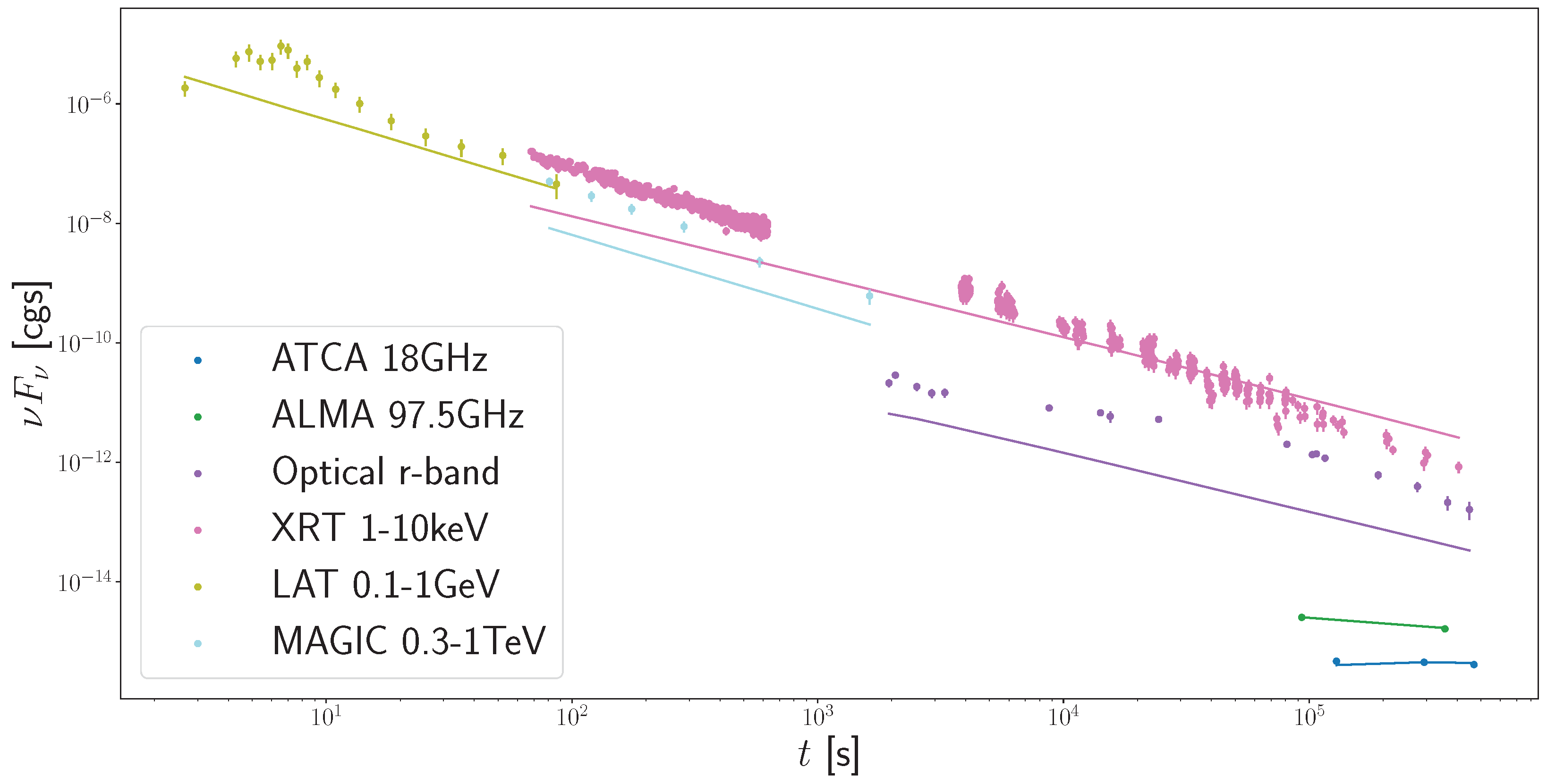
The data used in this analysis were taken from Figure 7 of [24]. These multi-wavelength observations in TeV, GeV gamma-rays, X-rays, optical, and radio were collected by the MAGIC telescope (0.3–1 TeV), Fermi-LAT instrument (0.1–1 GeV), Swift-XRT instrument (0.3–10 keV), and ALMA (97.5 GHz) and ACTA (18 GHz) antennas.

3. Theoretical Model

We use a state-of-the-art theoretical model presented in [37]. Using a physically motivated electron distribution based on first-principles simulations, we can compute the broadband emission from radio to TeV gamma rays. This model includes the synchrotron emission and considers the SSC radiation, including the Klein–Nishina regime. However, it is similar to the other models of synchrotron emission since here we use this theoretical model in a simplified manner without the SSC component in order to reduce the computational time required for the simulations involved. The parameters needed for the model are dictated by the hydrodynamics of the jet that is then constrained by the kinetic energy $E_{\mathrm{kin}}$ of the afterglow emission and the density medium, assumed constant, which sets the number density of protons being encountered by the forward shock. There are four parameters constraining the microphysics of electron distribution and photon production. The parameters ${ϵ}_e$ and ${ϵ}_b$ are the fractions of in-flowing kinetic energy placed in the electron and magnetic fields, respectively. The third microphysical parameter p governs the steepness of the shock-accelerated electron distribution, i.e., $dN/dE\propto E^{-p}$.

Table 1. Parameter definitions according to the theoretical model in Warren et al. [37].

Parameter	Definition	Units
$n_0$	the CBM (circumbust medium) density	${\mathrm{cm}}^{-3}$
$E_0$	isotropic energy equivalent	ergs
${ϵ}_e$	the electron energy fraction	-
${ϵ}_b$	the B-field energy fraction at the shock	-
p	the index of the electron energy power-law (PL) distribution	-

shows the five parameters to infer with the respective definitions. We perform inference in log scale for the first four parameters $n_0$, $E_0$, ${ϵ}_e$, and ${ϵ}_b$ and linear scale for p, which are defined in Table 1. The parameters $n_0$ and $E_0$ are the density for the constant medium ($n=n_0{\mathrm{cm}}^{-3}$) and the kinetic energy ($E_{\mathrm{kin}}=E_0\mathrm{erg}$), respectively.

As a first step, in this paper, we perform Bayesian parameter inference for the aforementioned model without the inclusion of the thermal distribution of electrons in the SSC. This is a rather crude simplification that allows us to reduce the computational time needed to numerically evaluate the likelihood function and hence gives us the opportunity to perform a thorough comparison between different inference methods. In the future, we would like to examine the model with the full SSC effects based on Bayesian inference procedures that allow for a reduction in the likelihood function calls, such as surrogate methods [41], or likelihood-free amortized methods based on Bayesian optimization [42] or neural networks [43,44].

4. Methodology

We perform Bayesian parameter inference using dynamic nested sampling (NS) [45,46,47], a commonly used algorithm in astrophysics. Nested sampling is a Monte Carlo algorithm for computing an integral over a model parameter space. In the context of Bayesian parameter inference with some data D, the integrand is the likelihood function $L\left(D\right|\mathit{\theta })$, which is marginalized over the parameters $\mathit{\theta }$ (a d-dimensional vector including all parameters of the model) according to the prior probability density $\rho \left(\mathit{\theta }\right)d\mathit{\theta }$, which gives a measure of the parameter space. Integrals over the posterior density, like the evidence $Z=\int L\left(D\right|\mathit{\theta }\left)\rho \right(\mathit{\theta })d\mathit{\theta }$, allow for insightful statements about what model parameter regions are probable or improbable. Exploring, navigating, and integrating these parameter spaces can exhibit many challenges. Nested sampling addresses these challenges and it makes computing Z practical for a wide variety of problems. Posterior samples are also obtained via NS during the computation of the evidence.

For more details, to solve the d-dimensional integral of the posterior distribution $P\left(\mathit{\theta }\right|D)$,

$$Z=\int \cdots \int L\left(D\right|\mathit{\theta })\rho \left(\mathit{\theta }\right)d{\theta }_1\cdots d{\theta }_d$$

(1)

NS transforms it into a one-dimensional integral. Suppose ${\widehat{\theta }}_1,\cdots ,{\widehat{\theta }}_N$ are independent and identically distributed samples from the prior, and their likelihoods are $L_1,\cdots ,L_N$. Let us assume the samples are indexed so that $L_1=L_{\lim }=\min \{L_1,\cdots ,L_N\}$. The survival function of a likelihood-restricted prior is

$$X\left(L_{\lim }\right)=\mathbf{Pr}\{L\left(D\right|\mathit{\theta })\le L_{\lim }\}={\int }_{L\left(D\right|\mathit{\theta })\le L_{\lim }}\rho \left(\mathit{\theta }\right)d\mathit{\theta }$$

(2)

Setting $L_1=L_{\lim }$ and repeating the sampling procedure with the prior restricted to $L\left(D\right|\mathit{\theta })\le L_{\lim }$ induces nested sampling. The recursion tracks an ever-shrinking X with an ever-increasing likelihood threshold $L_{\lim }$. Then, a “sorting” of the prior space via the likelihood function is achieved by the inverse:

$$Z={\int }_0^1{L}_{\lim }\left(X\right)dX$$

(3)

Note that the inverse of X, $L_{\lim }\left(X\right)$, is a monotonically increasing function.

For the implementation, we use the UltraNest (https://johannesbuchner.github.io/UltraNest/ accessed on 27 January 2024) package [48]. With a focus on correctness and speed, UltraNest is especially useful for multi-modal or non-Gaussian parameter spaces, computationally expensive models, in robust pipelines. It allows for fitting arbitrary models specified as likelihood functions written in Python, C, C++, Fortran, Julia, or R. It is especially remarkable that UltraNest is free of tuning parameters and theoretically justified: compared to many other NS packages, UltraNest implements better motivated self-diagnosing algorithms and improved, conservative uncertainty propagation.

We can contrast the nested sampling approach to posterior evaluation with the traditional Markov Chain Monte Carlo (MCMC) approach. MCMC is a very popular algorithm in Bayesian inference, which allows for one to sample from the posterior of a model’s parameter set. We have tested a popular MCMC implementation using the emcee (https://github.com/dfm/emcee accessed on 27 January 2024) package [49] with the same model and data in our study. The relevant differences between UltraNest and emcee that we want to mention are the following. While emcee is designed to work well for mono-modal posteriors without very fat tails, UltraNest can handle multi-modality out of the box. Furthermore, emcee requires MCMC convergence checks, which are tricky to get correct and can fail if the trajectories have not explored all the peaks of the posterior. In a previous study, Ryan et al. [50] used emcee to infer the posterior distributions of parameters of afterglow light curves.

In the implementation of our parameter estimation procedure, we assume that the data points are Gaussian random variables and we use a Gaussian likelihood. Therefore, our log likelihood is proportional to

$${\chi }^2=\sum {\left(\frac{m_i-y_i}{{\sigma }_i}\right)}^2,$$

(4)

where $m_i$ are simulated output values and $y_i$ are observed data points i, and ${\sigma }_i$ are standard deviations of the data point. We use the log likelihood computed as $logL=-{\chi }^2/2$.

5. Results

5.1. Definition of Priors

In Bayesian inference, we need to provide prior distributions for all the parameters to infer. We have five physical parameters and we start by defining the prior distributions for each of them. For the analysis with UltraNest, the typical range where parameters are allowed to vary are advised based on prior knowledge of the physical understandings of GRBs. For example, we are using a physical model that imposes a relation between the first two parameters, ${log}_{10}{n}_0$ and ${log}_{10}{E}_0$, such that the latter has to be larger than the former by a constant. For this reason, we impose a conditional prior enforcing $(C+{log}_{10}{n}_0-{log}_{10}{E}_0)<0$, where C is a constant that depends on the ending time of the simulation (given by the latest experimental observation) and the current theoretical model. Another relation we impose is that ${log}_{10}{ϵ}_e$ > ${log}_{10}{ϵ}_b$, because this is a typical situation in the physical model we are using. A summary of the priors defined for the UltraNest approach is reported in

Table 2. The prior used in the UltraNest parameter inference. The constant C is explained in the text, and for our model simulations it is set to $51.68$.

	Lower Bound	Upper Bound	Distribution
${log}_{10}{n}_0$	−3	3	uniform
${log}_{10}{E}_0$	$C+{log}_{10}{n}_0$	60	uniform
${log}_{10}{ϵ}_b$	−7	0	uniform
${log}_{10}{ϵ}_e$	${log}_{10}{ϵ}_b$	0	uniform
p	2	4	uniform

.

For the inference analysis with the MCMC algorithm implemented in emcee, we use the same data and the same model as we did with UltraNest, but we modify the prior to constrain the MCMC algorithm even further. The reason for this is to test a different workflow where priors are informed by preliminary numerical simulations of the model. We first remove any constraints between different parameters and therefore obtain a factorized prior of five uniform distributions. Then, we obtain the prior bounds by performing a scan of the log-likelihood landscape and identifying a region near the maximum using the gradient-free methods implemented in the Nevergrad (https://github.com/facebookresearch/nevergrad) package [51]. With gradient-free methods, one is allowed to select a computational budget that can be spent to explore the cost function’s landscape by running only the forward-shock model (in this case we run the model of Section 3 without the SSC component). The final prior defined for the emcee approach is reported in

Table 3. The prior used in the MCMC simulations.

	Lower Bound	Upper Bound	Distribution
${log}_{10}{n}_0$	−0.2	0.8	uniform
${log}_{10}{E}_0$	52.5	55.0	uniform
${log}_{10}{ϵ}_b$	−5.6	−3.5	uniform
${log}_{10}{ϵ}_e$	−1.2	−0.6	uniform
p	2.2	2.6	uniform

. Since this prior is different from the one used in the UltraNest approach, we will not draw a comparison of the parameters’ posterior between the two methods (since it will not be a fair comparison), but we will merely show that both approaches can be used in the analysis pipeline of GRB afterglows.

5.2. Posterior Results

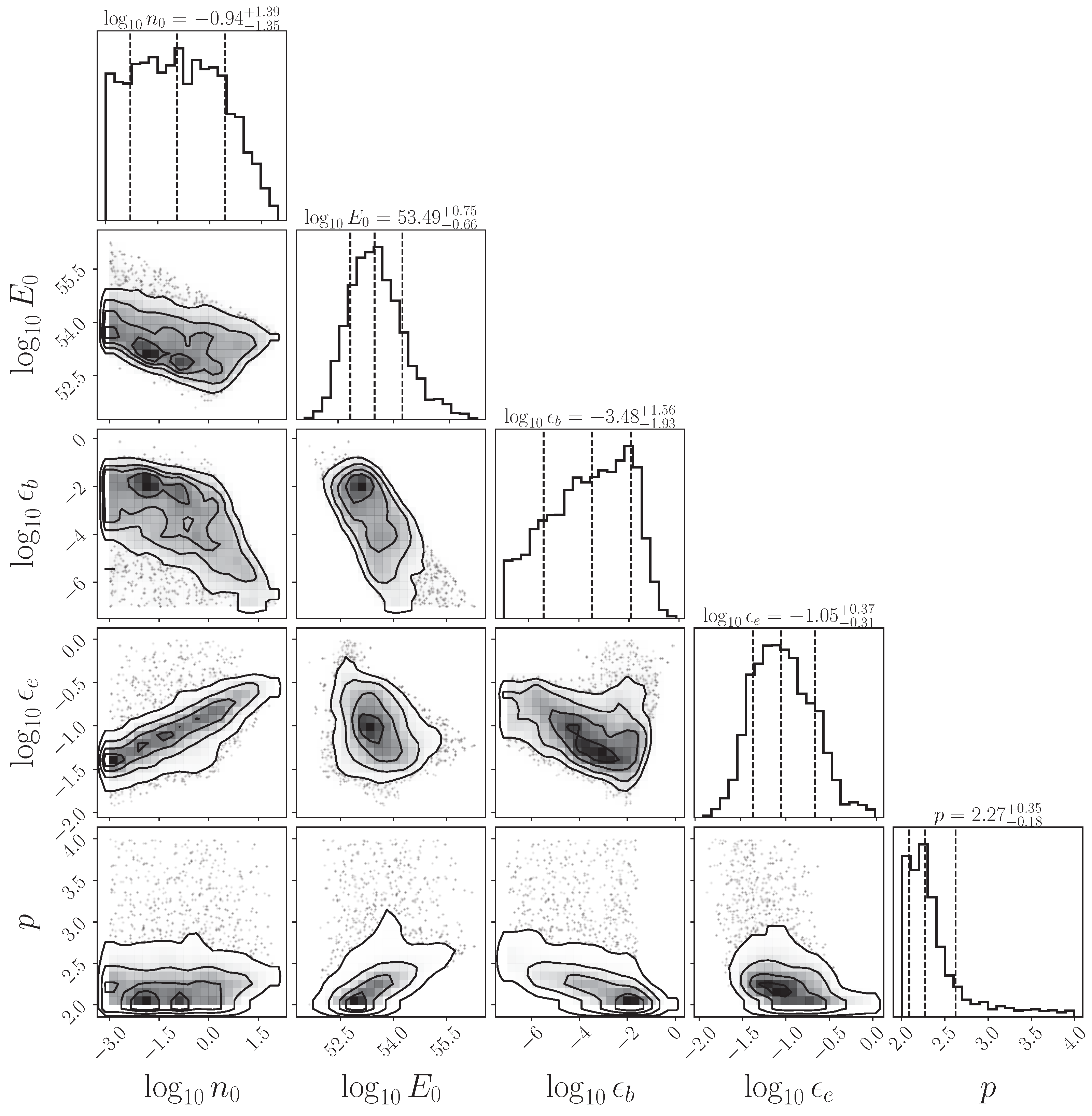
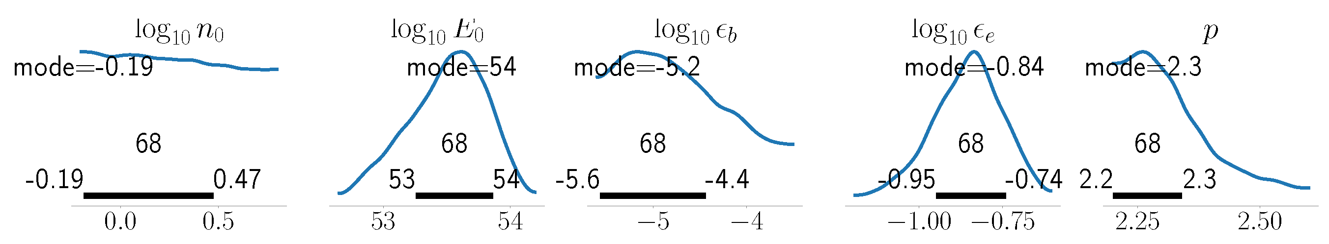
UltraNest performs nested sampling until a strict convergence criterion is satisfied on the calculation of the evidence Z. While iterating to convergence, posterior samples are collected and weighted. We plot those samples using a corner plot in Figure 1. The inferred parameter values using the UltraNest posterior are summarized in

Table 4. The inferred parameter values from the UltraNest posterior.

	Mean	Std. Dev.	3% (HDI)	97% (HDI)
${log}_{10}{n}_0$	−0.903	1.226	−2.999	1.063
${log}_{10}{E}_0$	53.547	0.738	52.201	54.947
${log}_{10}{ϵ}_b$	−3.621	1.561	−6.515	−1.182
${log}_{10}{ϵ}_e$	−1.027	0.328	−1.624	−0.454
p	2.386	0.388	2.005	3.216

.

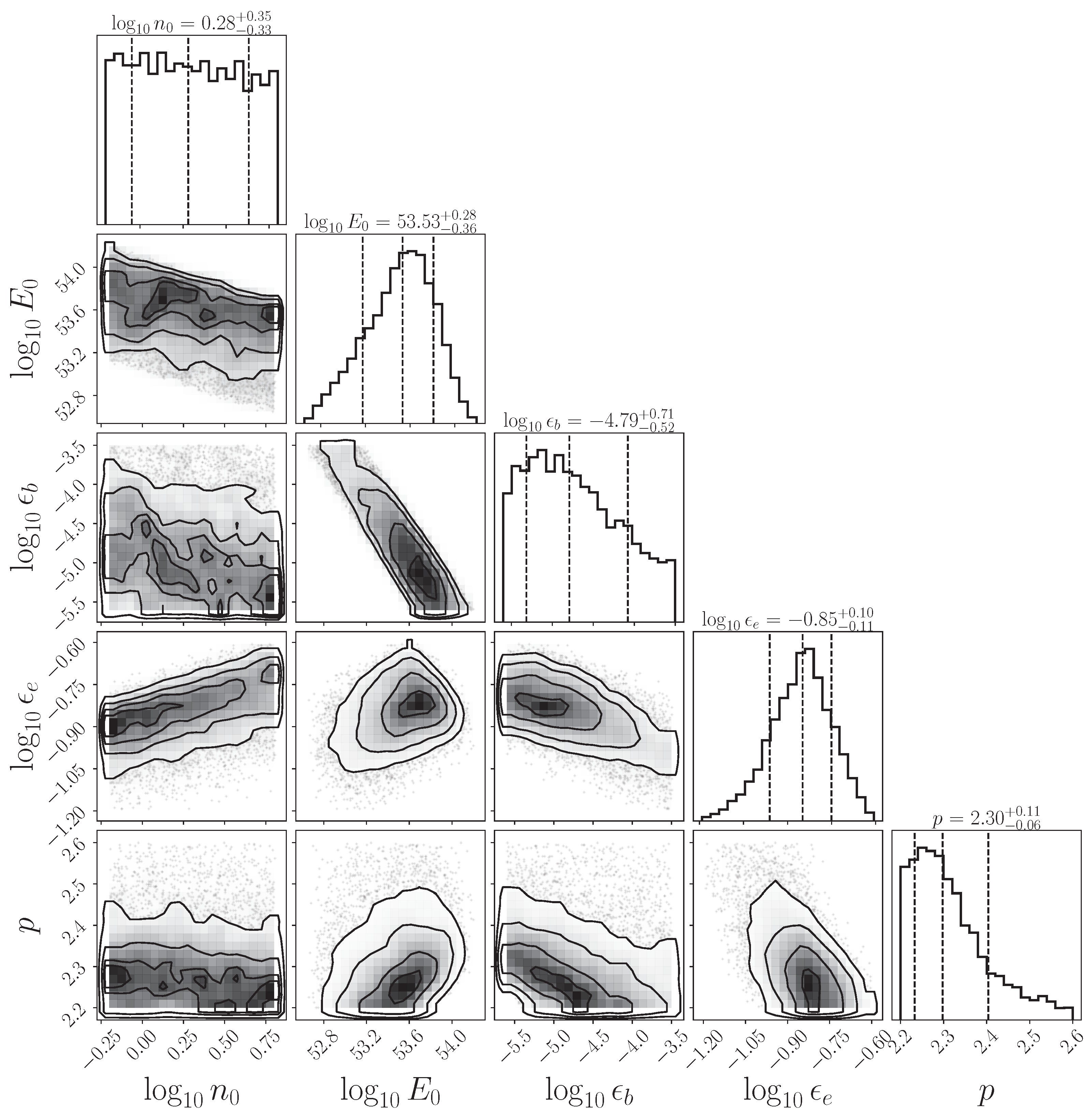
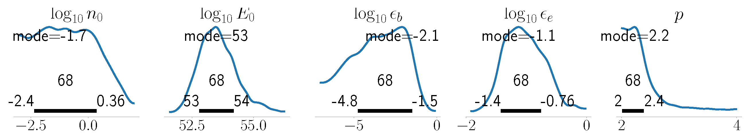
In the case of the emcee algorithm, an ensemble of trajectories (walkers) is used to explore the posterior probability density and to draw samples from it. The corner plot for the posterior samples from the emcee iterations is shown in Figure 2. The inferred parameter values from this posterior are summarized in

Table 5. The inferred parameter values of MCMC simulations. This summary is computed after the burn-in time of each chain is discarded and after removing correlated samples along the chains.

	Mean	Std. Dev.	3% (HDI)	97% (HDI)
${log}_{10}{n}_0$	0.288	0.288	−0.199	0.737
${log}_{10}{E}_0$	53.502	0.301	52.893	54.004
${log}_{10}{ϵ}_b$	−4.721	0.554	−5.600	−3.753
${log}_{10}{ϵ}_e$	−0.856	0.104	−1.056	−0.661
p	2.318	0.088	2.200	2.492

. One difference between this MCMC-based algorithm and the nested sampling algorithm is that we need to compute diagnostic quantities to assess the reliability of the trajectories used to explore the posterior. If these quantities suggest that there are no issues with the MCMC algorithm such as long autocorrelation times, poor effective sampling rates, or even convergence issues, we can then use the posterior samples to reliably compute confidence intervals for our model parameters. Information about the diagnostic quantities for the MCMC simulations is reported in

Table 6. The diagnostic quantities for the MCMC simulations. The diagnostic properties are computed after the burn-in time of each chain is discarded and after removing correlated samples along the chains.

	Mean	Std. Dev.	ESS	ESS	$\widehat{\mathit{R}}$
	(MCSE)	(MCSE)	(Bulk)	(Tail)
${log}_{10}{n}_0$	0.006	0.004	2603	4768	1.00
${log}_{10}{E}_0$	0.006	0.004	2625	4099	1.00
${log}_{10}{ϵ}_b$	0.011	0.008	2545	4779	1.00
${log}_{10}{ϵ}_e$	0.002	0.002	2367	4139	1.00
p	0.002	0.001	2164	3265	1.00

.

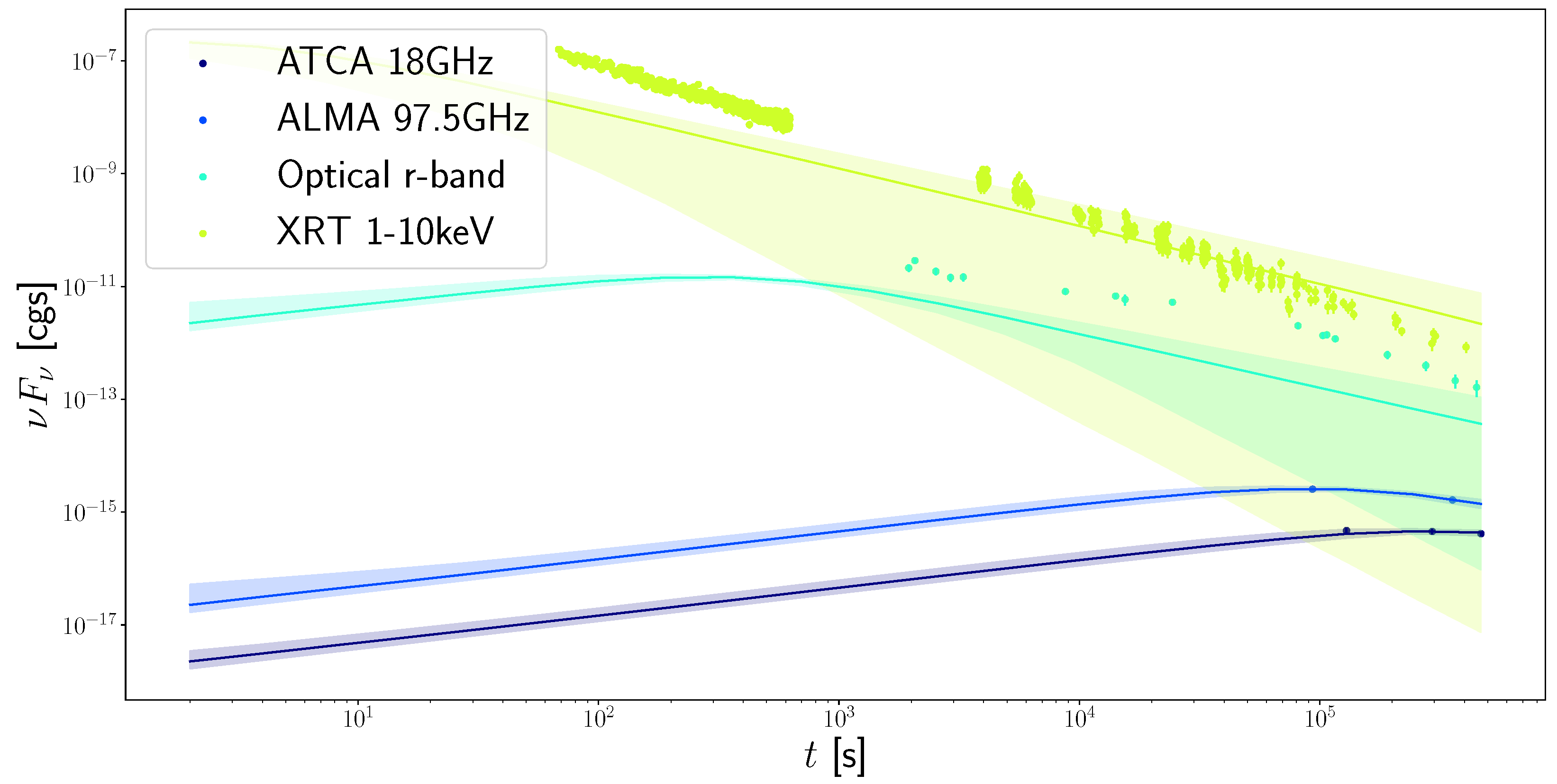
5.3. Light Curves

After the parameter inference in this Bayesian framework, we can proceed to perform posterior predictive checks: we can take parameter sets directly from our inferred posterior and we can use them in our physically motivated model to generate a set of light curves in different frequency bands. Moreover, using several parameter samples from the posterior gives us access to a robust uncertainty evaluation of the predicted light curves.

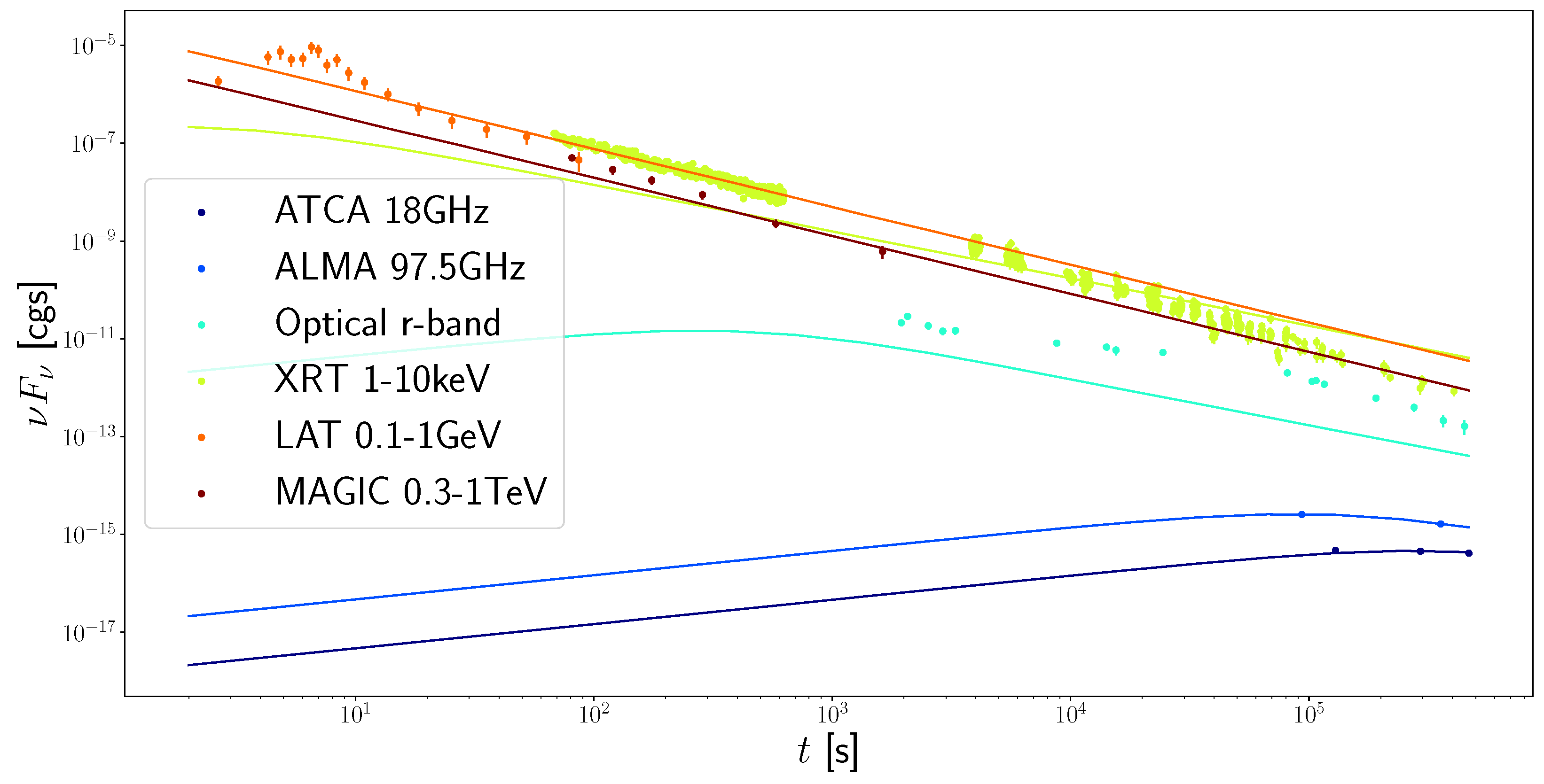
We set up the curves corresponding to the maximum likelihood parameters, which are reported by the UltraNest algorithm. These values are ${log}_{10}{n}_0=-0.7442,{log}_{10}{E}_0=53.8623,{log}_{10}{ϵ}_b=-4.4042,{log}_{10}{ϵ}_e=-0.9754,p=2.2516.$ The plotted results are in Figure 3. Similar light curves can be obtained following the same procedure in the case of the emcee algorithm, which are reported in Appendix A in Figure A3.

We do see deviations between the data and the curves coming from our maximum likelihood parameters. This is expected due to the simplified nature of the model used during the parameter inference procedure. Future works will explore the inference in the full model, which includes an SSC component to model high-energy photons more accurately.

In [24], the high-energy radiation (TeV, GeV, and X-ray) was fitted with a model optimized in that domain, and a least-squares curve-fitting procedure determined the following parameters: $k=0$, ${ϵ}_e=0.07$, ${ϵ}_b=8\times {10}^{-5}$, $p=2.6$, $n_0=0.5$, and $E_{\mathrm{kin}}=8\times {10}^{53}$ erg. The effect of the total flux (synchrotron and SSC) and the SSC contribution were shown by the solid lines and dashed line. At lower frequencies, the authors had opted for a different model, which in turn fails to explain the behavior of the TeV light curve; the low-energy model parameters are $k=2$, ${ϵ}_e=0.6$, ${ϵ}_b={10}^{-4}$, $p=2.4$, $A_{\mathrm{W}}=0.1$, and $E_{\mathrm{kin}}=4\times {10}^{53}$ erg. These two sets of model parameters are a baseline result for the procedures we followed in our study. The key difference is that we are using a single model that, in its full form, would allow us to reproduce the light curves over the entire energy range of the GRB afterglow photons. Moreover, with Bayesian inference we would also obtain the full correlated uncertainty quantification on the parameters of the model.

We remark one more time that the results we are presenting here come from a simplified model that can be studied with limited computational resources and it is not expected to reproduce the full energy range even if the optimal parameters are found.

5.4. Uncertainty

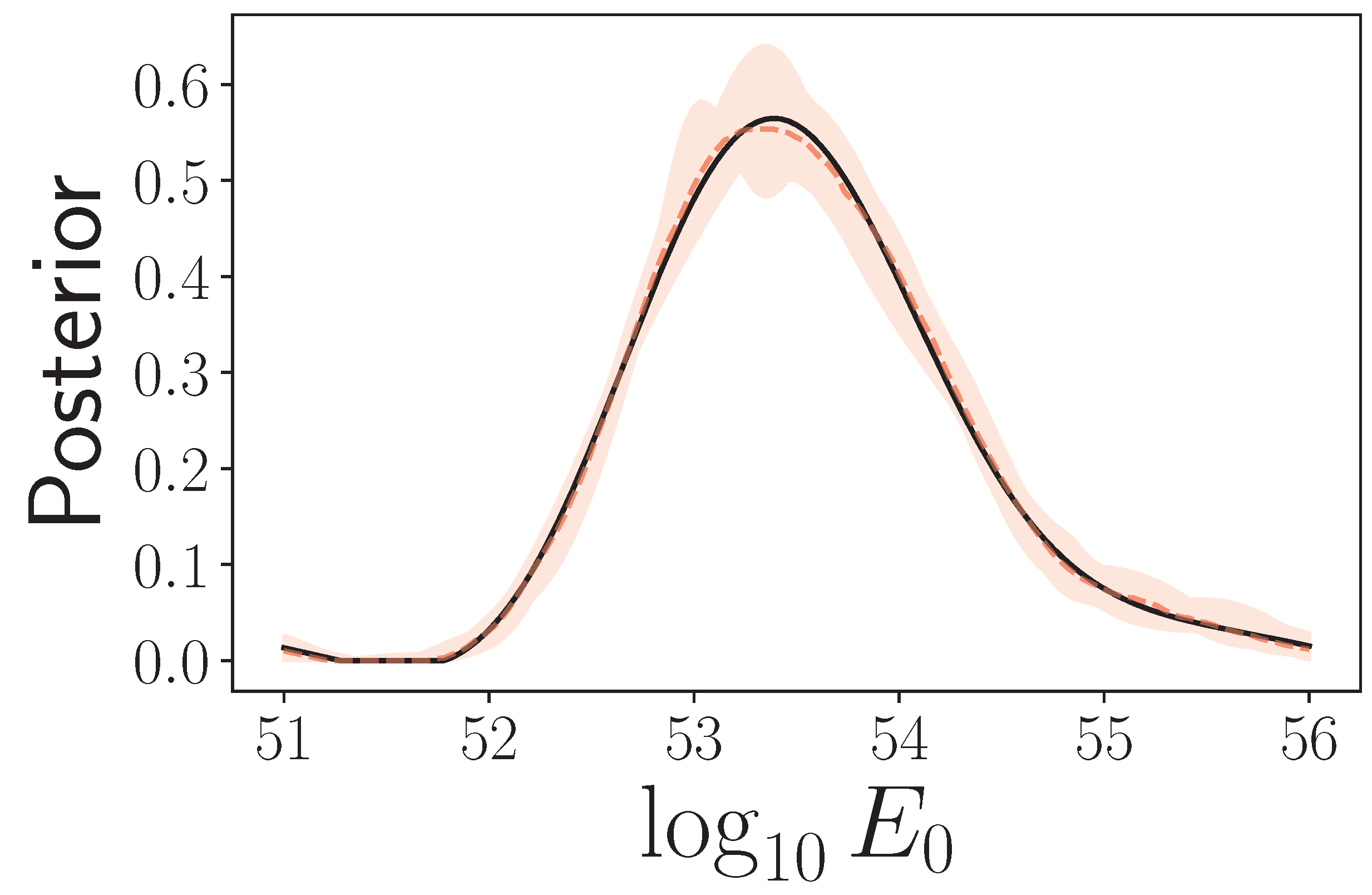
Here, we briefly comment on the uncertainty quantification capabilities of the full Bayesian framework. In Figure 4, we show the uncertainty of the parameter ${log}_{10}{E}_0$ coming from the UltraNest algorithm. The red dashed line is the central value of the bootstrapped posterior samples, while the black line is the empirical distributions of the samples only: they are in good agreement. The uncertainty from the $99\%$ percentile interval of the bootstrap samples is very small. A similar result is obtained for the remaining four parameters. In addition, we plotted the uncertainty on the light-curve fitting in Figure 5 by adding a shaded region to represent the $99\%$ confidence intervals on the curves. One can see that the ATCA and ALMA bands have very accurate predictions with low uncertainties. The optical r-band light curve has high certainty at early times during the afterglow, but in the tail the prediction becomes less certain. For the XRT band, the uncertainty range is the widest, which might be due to the fact that this energy range is more susceptible to uncertainties in the parameters. Including these prediction error bands, we can see that the optical data are poorly modeled by our posterior parameters. In addition, the XRT data at early times $t<{10}^3$ s are outside the error bands. We will discuss these results and their implications in the next section.

5.5. Discussion on Simulations

The error bars in ATCA and ALMA are extremely small compared to other bands, which dominates the inference to fit these two bands first. In other words, different levels of error bars give the bands different importance or priorities in inference, since we are calculating the summed likelihood value. The sources of the error bars are different from band to band, because they are usually observed by different instruments and/or observatories. This is an important problem in studying GRBs, where the way of estimating observational uncertainties can drastically affect the conclusions of afterglow models and inherently slow our progress in understanding the origin of these important phenomena.

Without SSC, as expected, we cannot fit the bump in LAT data. This also confirms that SSC is needed to explain the behavior of high-energy bands. Our current results set a new baseline for this specific afterglow model from Warren et al. [37], and future work will address the parameter inference for the full model, where one expects a better light-curve fitting in high-energy bands. In particular, we expect that a better model is needed in order to simultaneously fit the high-energy data and the optical and r-band data, currently poorly fitted as shown in Figure 5. When the radio data are removed, it is possible for the model to fit the XRT and optical data quite accurately.

5.6. Implications and Discussion

We now analyze the results we obtained from the parameter inference with the UltraNest algorithm and we compare them to what is available in the previous literature. This is a necessary step in order to draw physical conclusions about our analysis, but we note that we are using a simplified model of the afterglow that does not capture the correct physics of the very energetic photons. In the following we use the values reported in the titles of the diagonal panels of the corner plot in Figure 1, representing the 0.5 quantile and the deviation from the 0.16 and the 0.84 quantiles, with the corresponding sign.

The best-fit values of the microphysical parameters ${ϵ}_b={10}^{-{3.48}_{-1.93}^{+1.56}}$ and ${ϵ}_e={10}^{-{1.05}_{-0.31}^{+0.37}}$ lie in the range of values used to describe the multi-wavelength afterglow observations in some GRBs, ${10}^{-5}\le {ϵ}_b\le {10}^{-1}$ [23,52,53,54,55], and also in GRB 190114C [10,28,30,33,36]

The best-fit values of $n_0={10}^{-{0.94}_{-1.35}^{+1.39}}{\mathrm{cm}}^{-3}$ lie in the range of values reported as modeling the multi-wavelength afterglow observations of GRB 190114C [5,28,30,31,32] and of typical ones reported for a highly energetic burst [6,7,56]. Given the intrinsic column galaxy $N_H\simeq 8\times {10}^{22}{\mathrm{cm}}^{-2}$[57], the value of the circumburst medium supports the idea that the host might be an irregular galaxy, which has a size of ∼$20\mathrm{kpc}$.

Fraija et al. [28] derived the LAT-detected photons with energies larger than (≥100 MeV) and with probabilities $>90$% of being associated with GRB 190114C. This burst exhibited in the LAT data five photons with energies larger than 10 GeV and the highest-energy photon was 21 GeV detected at 21 s after the trigger time. The energetic LAT photons above 10 GeV have energies of 10, 21, 19, and 11 GeV and are detected at 18, 21, 36, and 65 s, respectively, after the GBM trigger (see the panel below in Figure 1 from Fraija et al. [28]). Given the best-fit values of the circumburst density and kinetic energy, and following the procedure described in [58] about the maximum energy radiated by the synchrotron forward-shock model, the maximum energies of this process at 18, 21, 36, and 65 s are 7.4, 7.1, 5.7, and 4.6 GeV, respectively.

We show from the fit that the simplified model cannot account for energies above 10 GeV, which indeed can be hardly interpreted in the standard synchrotron forward-shock model. The other LAT-detected photons can be successfully interpreted via the synchrotron model from the forward-shock model.

The best-fit values of the isotropic kinetic energy $E_0={10}^{{53.49}_{-0.66}^{+0.75}}\mathrm{erg}$ and the circumburst density $n_0={10}^{-{0.94}_{-1.35}^{+1.39}}{\mathrm{cm}}^{-3}$ lead to a value of the bulk Lorentz factor during the deceleration phase of $\mathsf{\Gamma }\approx 526$ at $10\mathrm{s}$. This value is comparable to those reported by other bursts that the Fermi-LAT has detected [14,28,56,59,60,61,62,63].

The efficiency $\eta \equiv E_{\gamma ,iso}/(E_{\mathrm{kin}}+E_{\gamma ,iso})$ offers very useful insight into the gamma-ray emission mechanism. The best-fit values of the equivalent kinetic energy $E_0={10}^{{53.49}_{-0.66}^{+0.75}}\mathrm{erg}$ and the isotropic energy in gamma rays ($E_{\gamma ,iso}$) reported by the GBM and LAT instruments during the prompt episode in the range of $E_{\gamma ,iso}=(3.5\pm 0.1)\times {10}^{53}\mathrm{erg}$[64] lead to a kinetic efficiency of $\approx 0.3$, which is in the range of those values reported in the literature [65,66,67].

The values of the spectral breaks derived from the best-fit parameters are $h{\nu }_{\mathrm{m}}^{\mathrm{ssc}}=2.5\times 10\mathrm{GeV}$, $h{\nu }_{\mathrm{c}}^{\mathrm{ssc}}=6.8\times {10}^2\mathrm{GeV}$, $h{\nu }_{\mathrm{KN},\mathrm{m}}^{\mathrm{ssc}}=9.8\mathrm{TeV}$, and $h{\nu }_{\mathrm{KN},\mathrm{c}}^{\mathrm{ssc}}=8.7\mathrm{TeV}$ and show that the KN effects are neglected.

The best-fit values of the parameters lead to synchrotron spectral breaks ${\nu }_{\mathrm{m}}^{\mathrm{syn}}=2.5\times {10}^{17}\mathrm{Hz}$, ${\nu }_{\mathrm{c}}^{\mathrm{syn}}=4.8\times {10}^{16}\mathrm{Hz}$, ${\nu }_{\mathrm{a}}^{\mathrm{syn}}=5.7\times {10}^8\mathrm{Hz}$ for ${\nu }_{\mathrm{a}}^{\mathrm{syn}}<{\nu }_{\mathrm{c}}^{\mathrm{syn}}<{\nu }_{\mathrm{m}}^{\mathrm{syn}}$, ${\nu }_{\mathrm{a}}^{\mathrm{syn}}=6.3\times {10}^{12}\mathrm{Hz}$ for ${\nu }_{\mathrm{m}}^{\mathrm{syn}}<{\nu }_{\mathrm{a}}^{\mathrm{syn}}<{\nu }_{\mathrm{c}}^{\mathrm{syn}}$, and ${\nu }_{\mathrm{a}}^{\mathrm{syn}}=1.3\times {10}^9\mathrm{Hz}$ for ${\nu }_{\mathrm{a}}^{\mathrm{syn}}<{\nu }_{\mathrm{m}}^{\mathrm{syn}}<{\nu }_{\mathrm{c}}^{\mathrm{syn}}$, which display that the synchrotron model lies in the weak absorption regime.

6. Summary and Conclusions

We have tested a model that adopts a physically motivated electron distribution based on first-principles simulations. We have computed the broadband emission from radio to TeV gamma rays. We have inferred five physical parameters from this afterglow model for the GRB 190114C. We use Bayesian inference to constrain the five main model parameters: the particle density, n; the equivalent kinetic energy, $E_{\mathrm{kin}}$; the microphysical parameters, namely, the electron distribution (${ϵ}_e$, ${ϵ}_b$); and the slope of the electron spectral distribution, p. This analysis is a case study to show how the GRB inference methodology can be carried out and explore the full parameter space. We used an advanced nested sampling algorithm called UltraNest, designed to invest computation to obtain a gold-standard exploration of the entire posterior distribution in one run for potentially complex posteriors. UltraNest implements self-diagnosing algorithms, and improved, conservative uncertainty propagation, which prioritizes robustness and correctness. We have compared the results between the standard MCMC algorithm and UltraNest, providing a first baseline for this afterglow model. We have shown that (i) the microphysical parameters, electron spectral index, kinetic efficiency, circumburst density, and bulk Lorentz factor lie in the range of values used to describe the multi-wavelength afterglow observations of other LAT-detected bursts (e.g., see [58,68]) and (ii) the four photons above ≳10 GeV cannot be interpreted in the standard synchrotron forward-shock model and below can be successfully interpreted by the synchrotron afterglow model. These can be explained via the SSC mechanism from the forward-shock model.

Possible future work can be to run the model parameter inference procedure with the SSC option and see how it changes the resulting parameter posterior distributions and the corresponding light-curve fitting in high-energy bands. One thing that hinders the simulation of the model with the SSC component is the computational costs, which might take several months even with supercomputer resources. To accelerate the computation, we have the idea to use neural network (NN) surrogates as the afterglow model. In this way, the NN acts as an approximation of the model with similar input and output values but with a much faster speed during the forward-shock (inference) pass. Another direction is to try using a different model with the same data and with the UltraNest algorithm to see how different modeling can affect the inferred parameters.