
Unveiling the Evolutionary State of Three B Supergiant Stars: PU Gem, ϵ CMa, and η CMa
 , , , , and
Abstract
:1. Introduction
2. Target Selection and Parameters Values from Literature
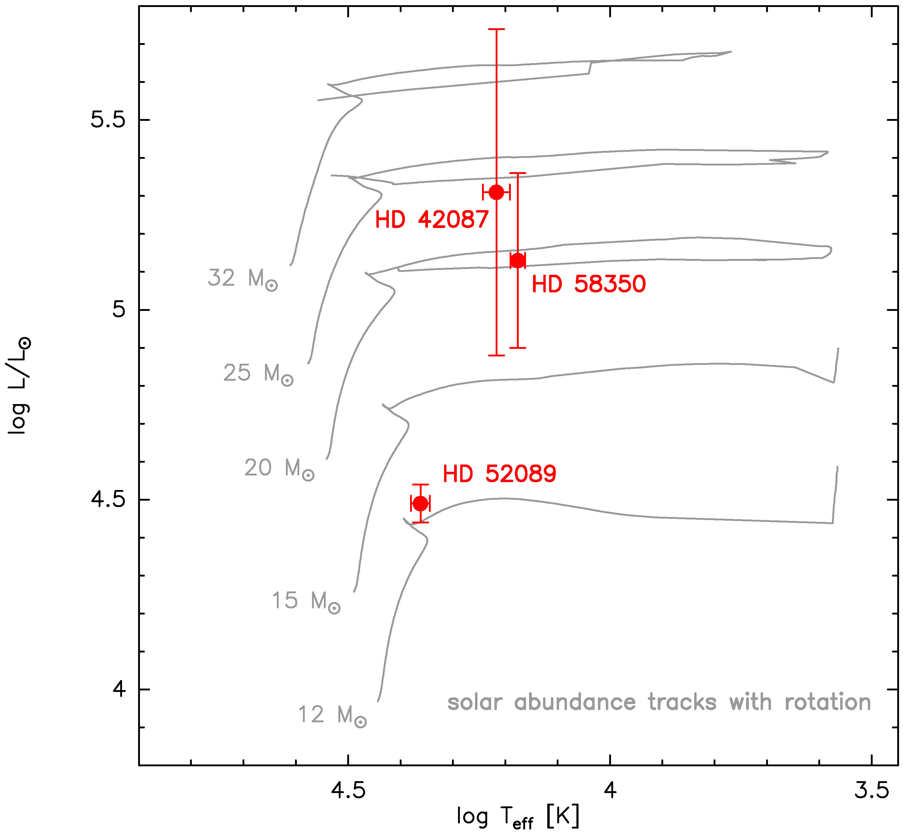
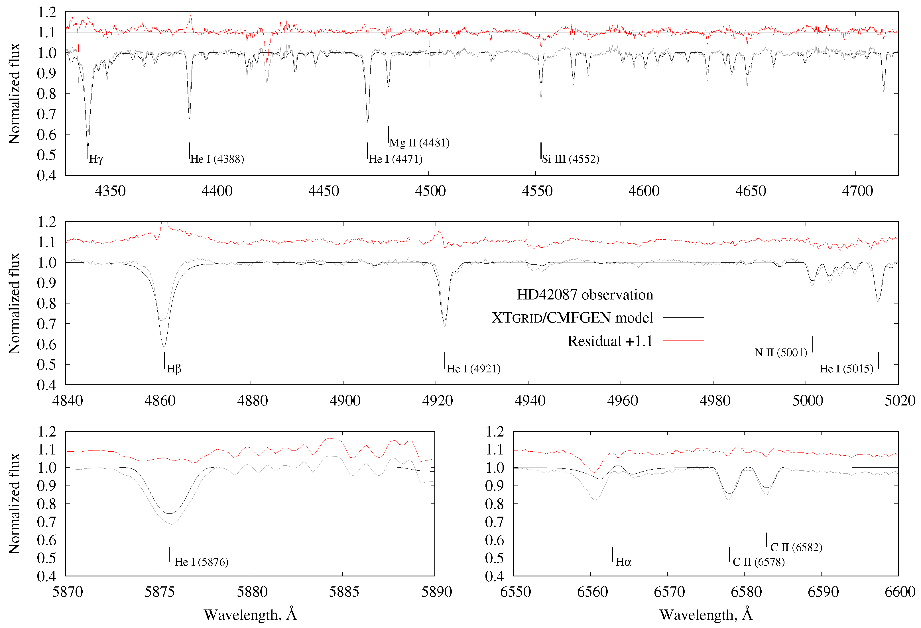
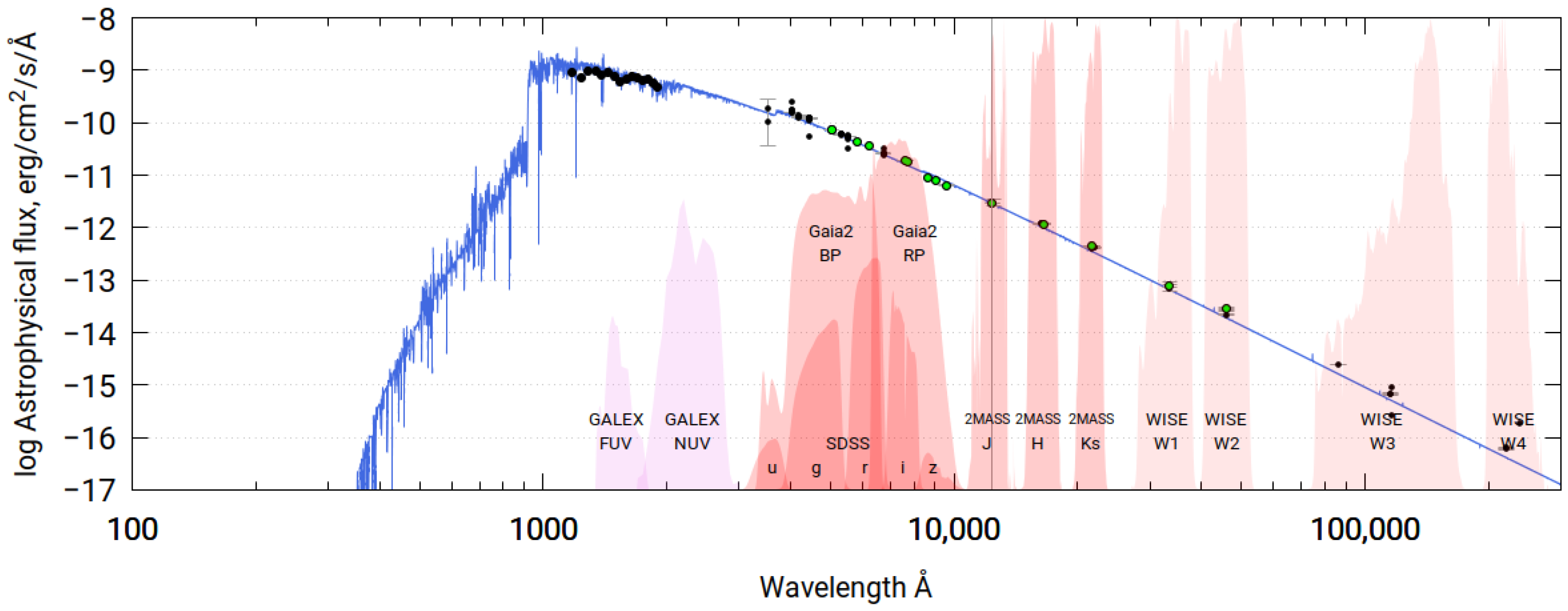
2.1. HD 42087
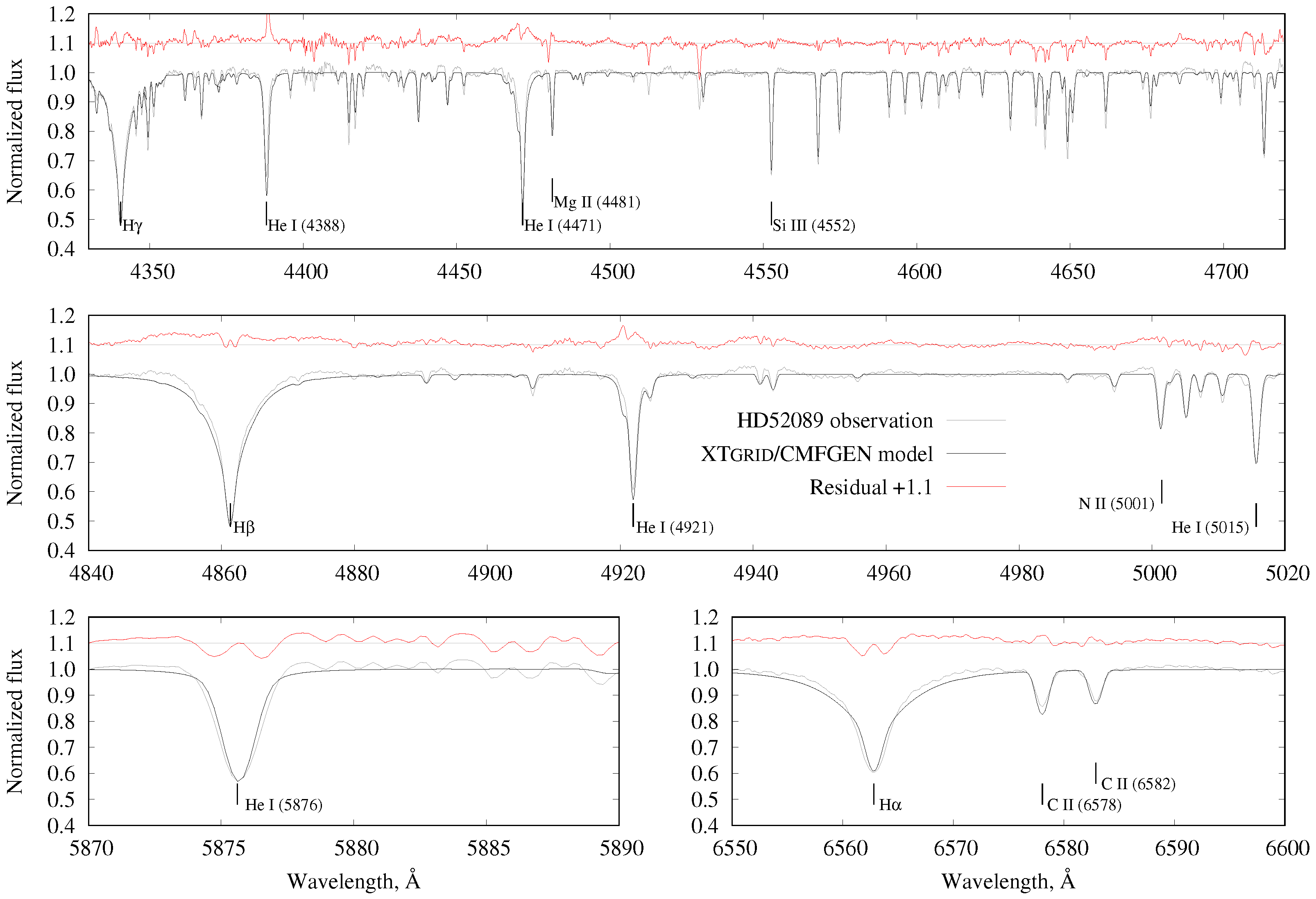
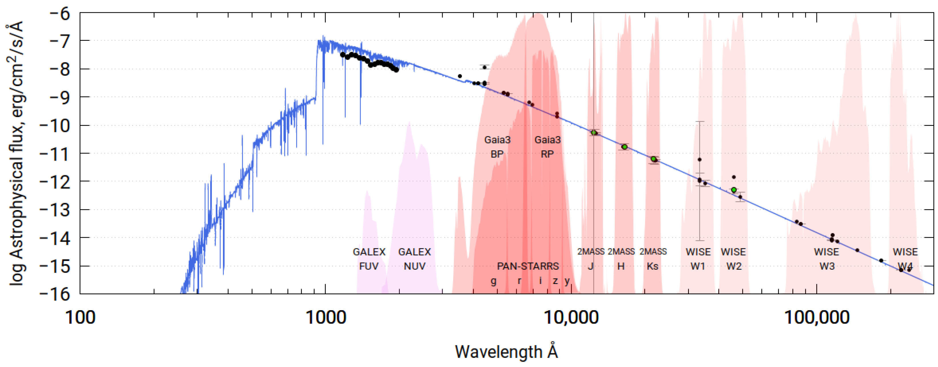
2.2. HD 52089
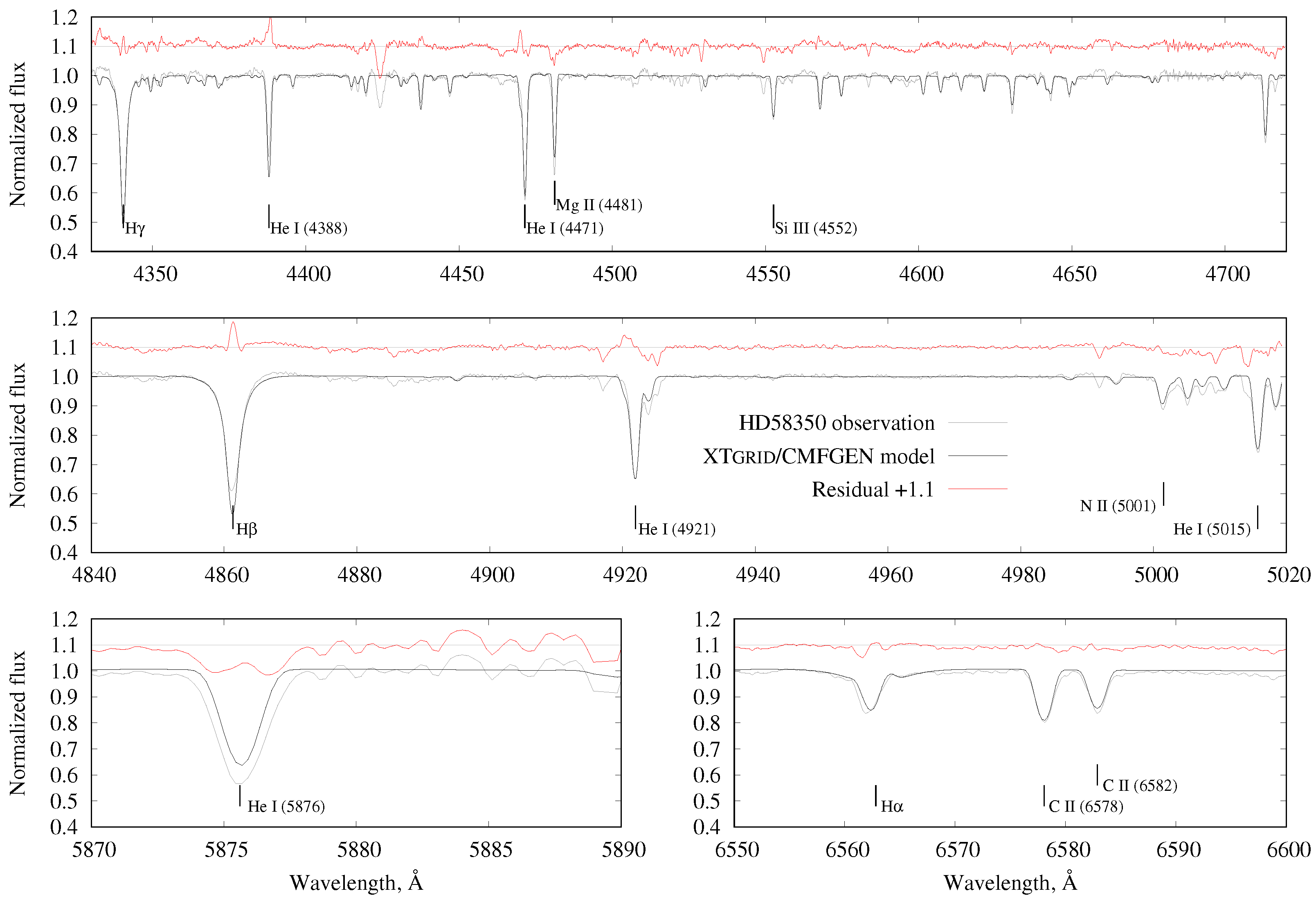
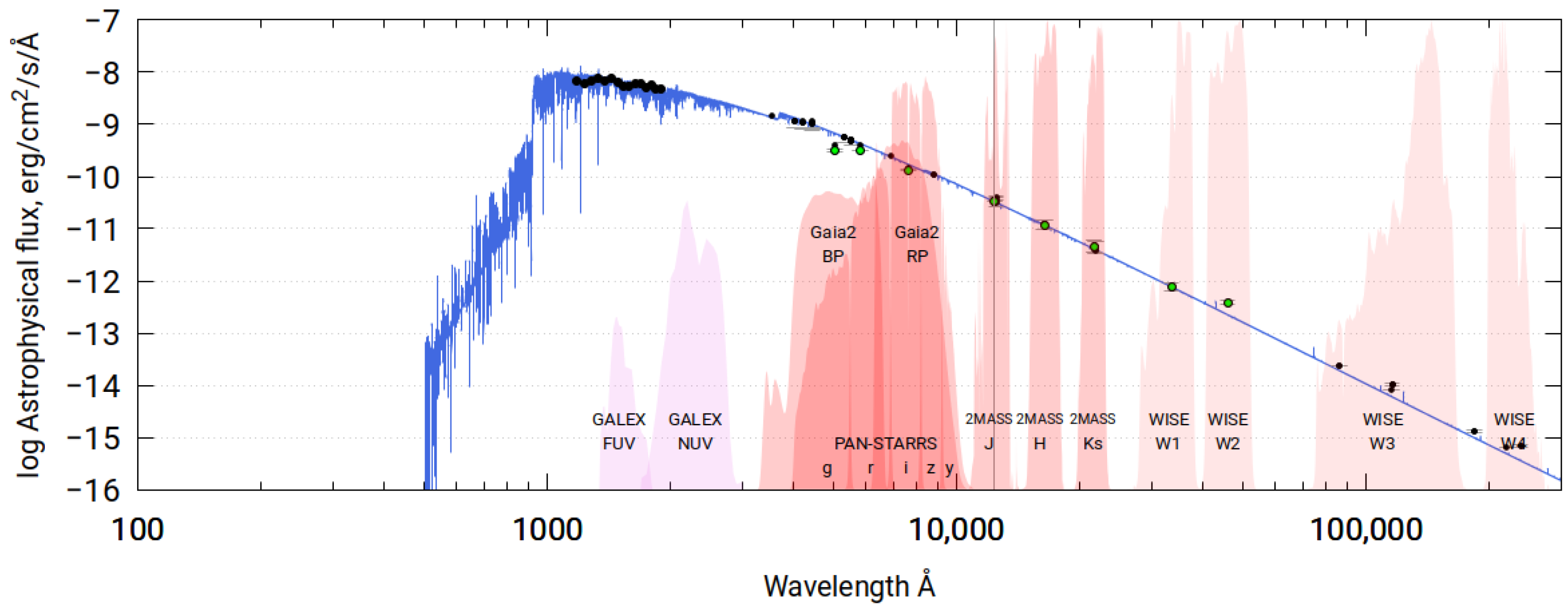
2.3. HD 58350

3. Observations
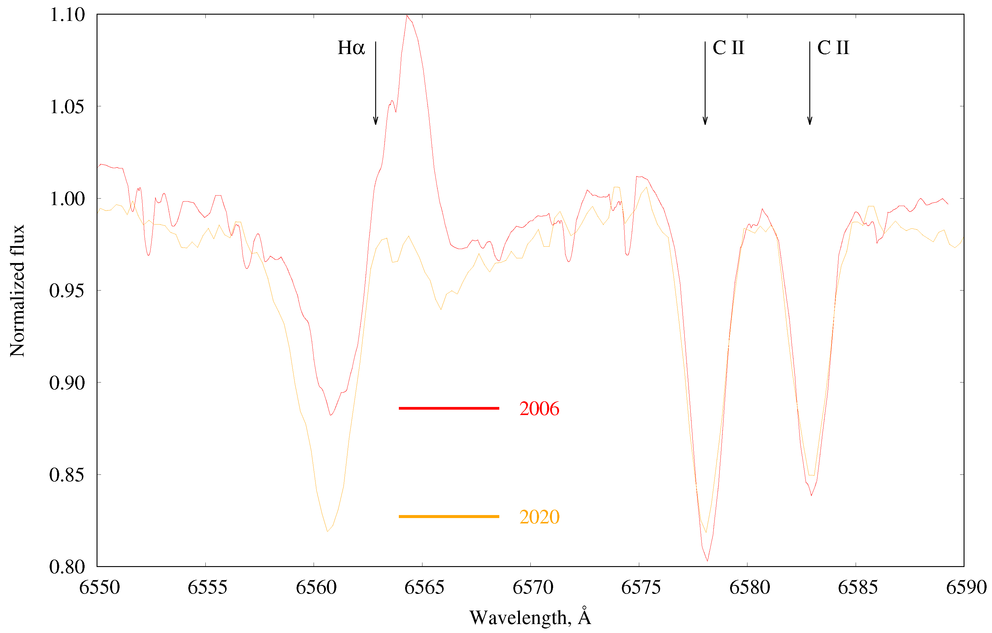
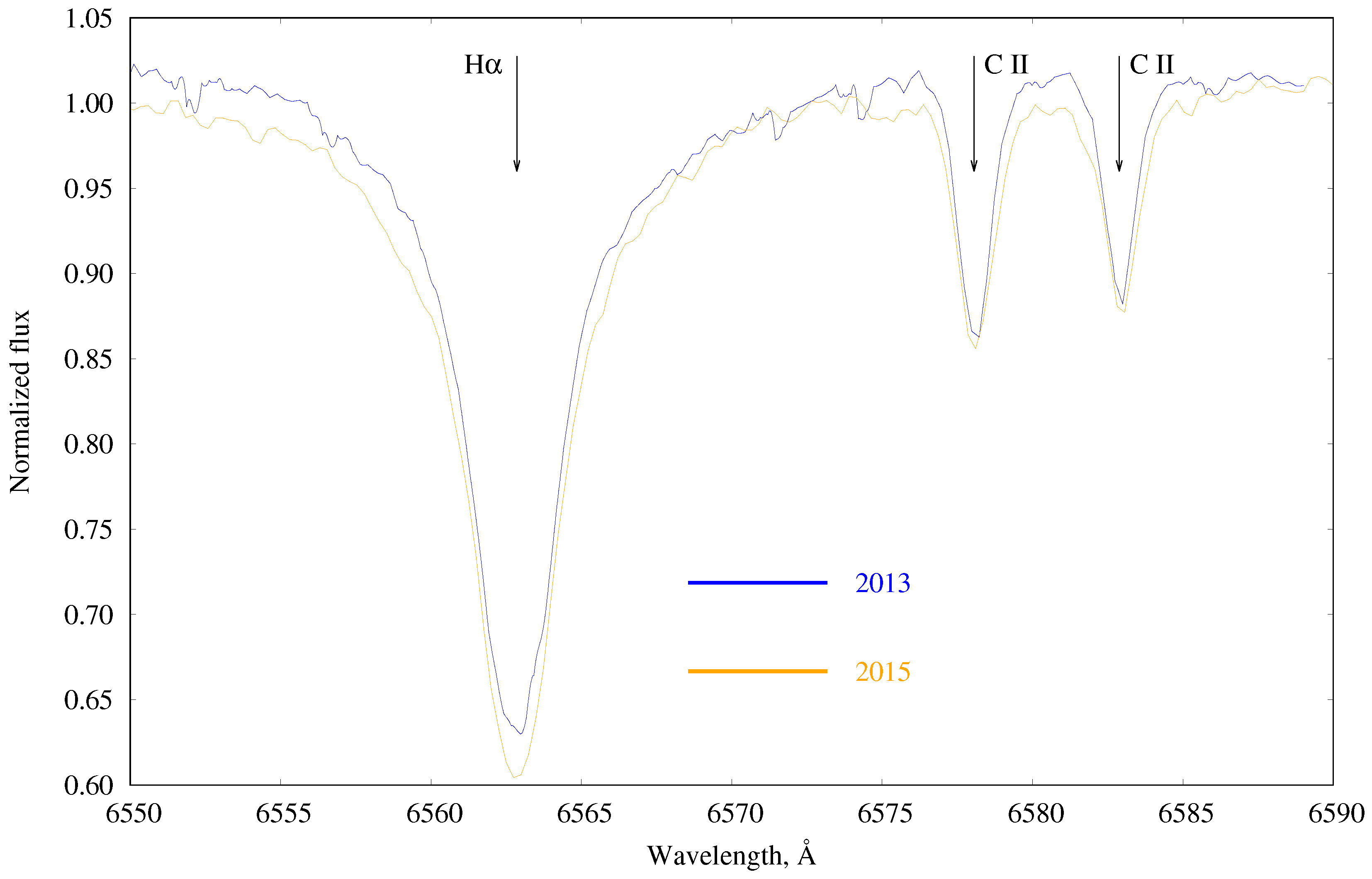
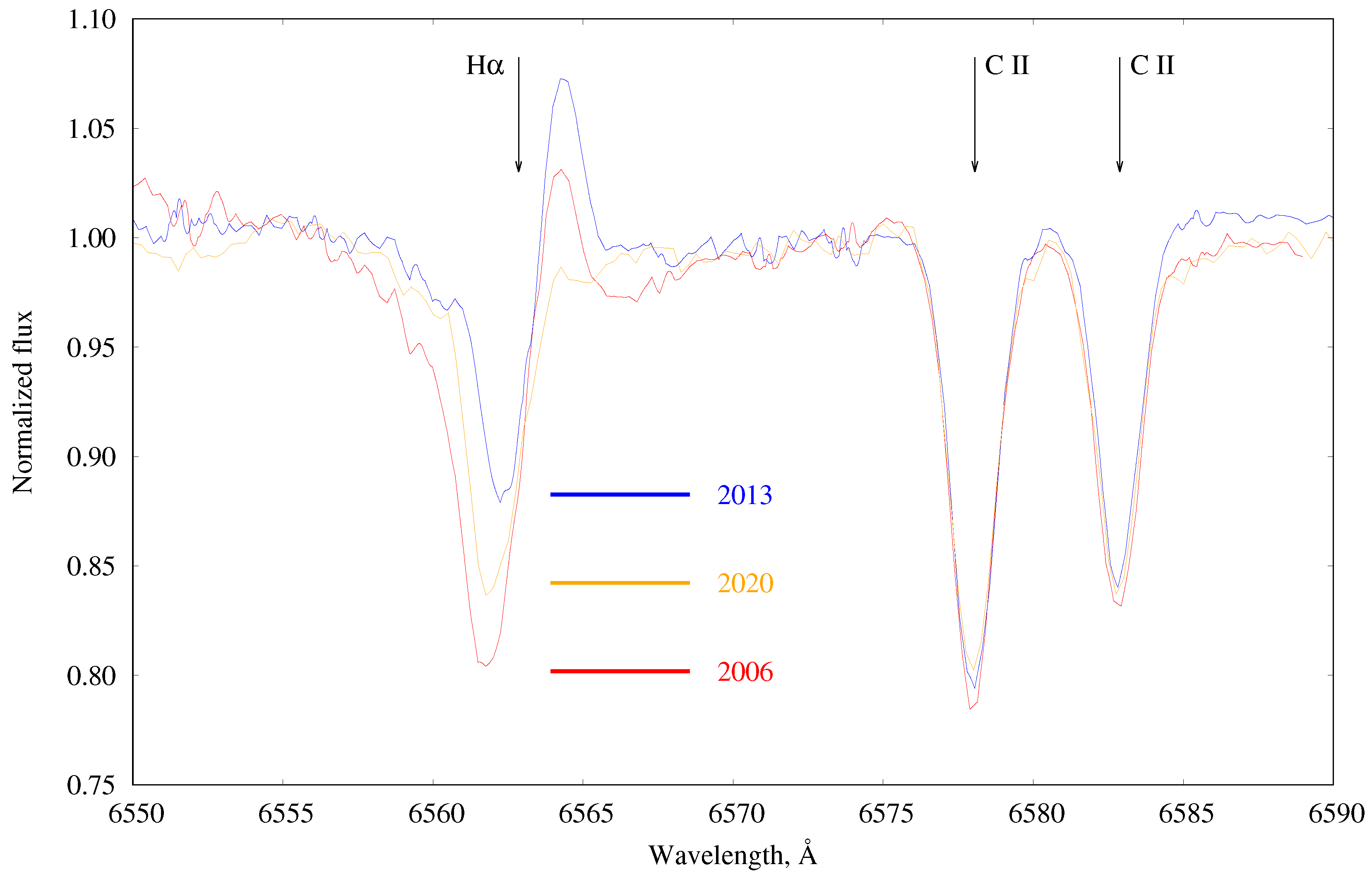
3.1. Spectra
3.2. Photometric Light Curves
4. Frequency Analysis
4.1. HD 42087
4.2. HD 52089
4.3. HD 58350
5. Modeling Tools for Spectral Analysis
5.1. The Code CMFGEN
5.2. Spectral Analysis with XTgrid
6. Discussion
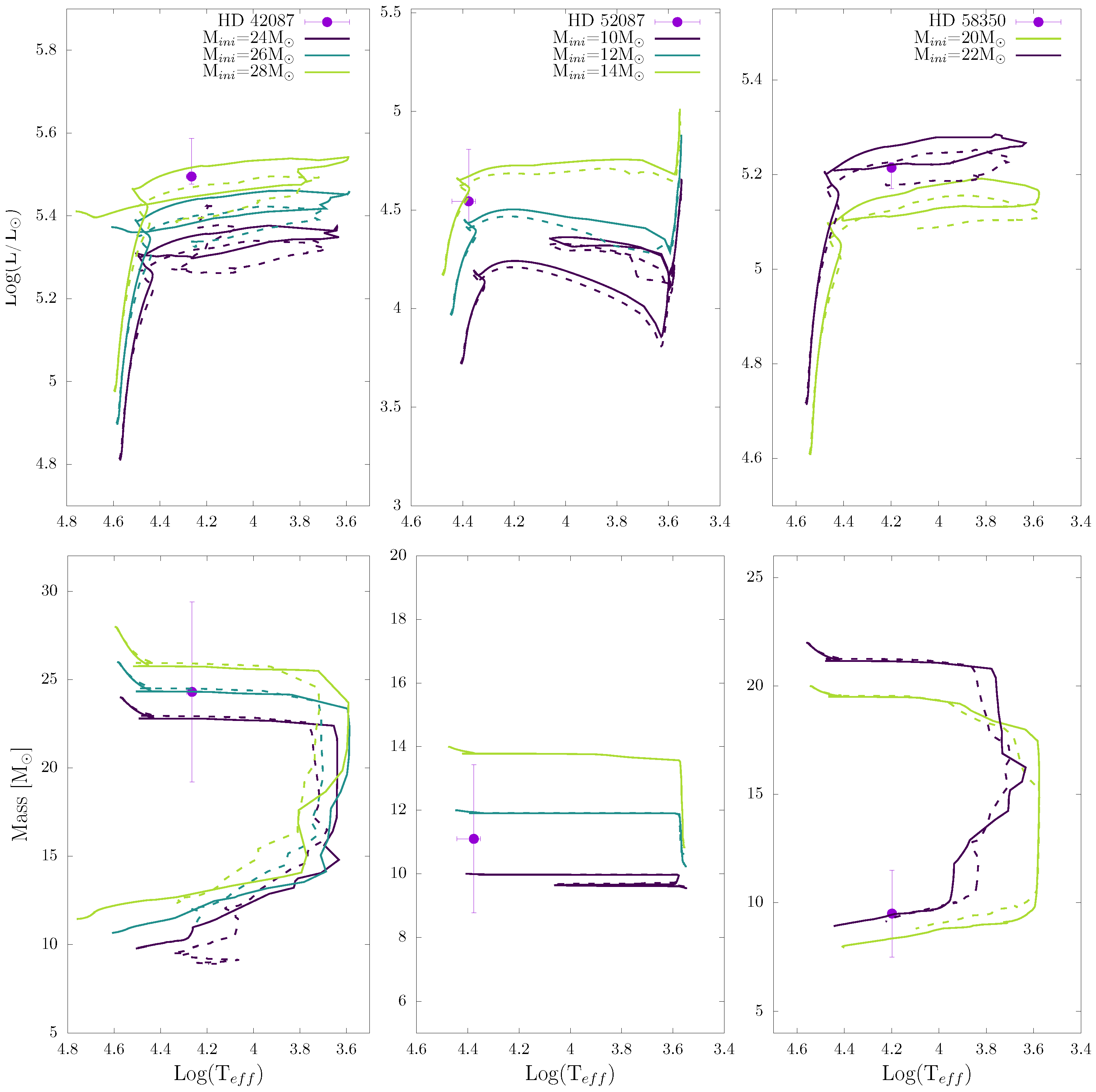
6.1. HD 42087
6.2. HD 52089
6.3. HD 58350
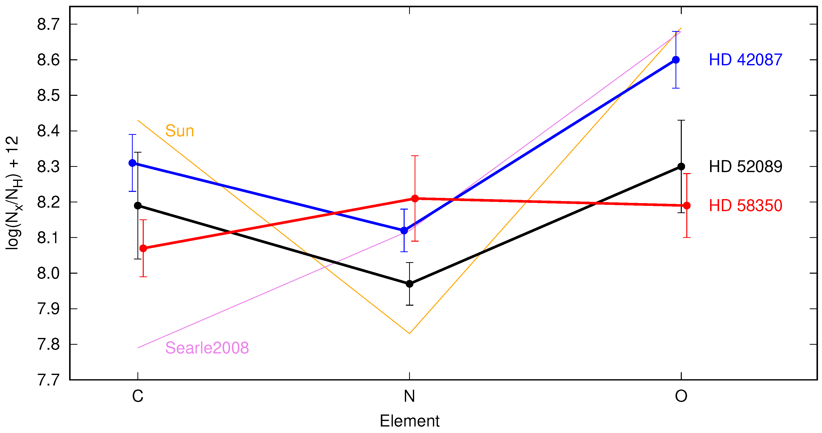
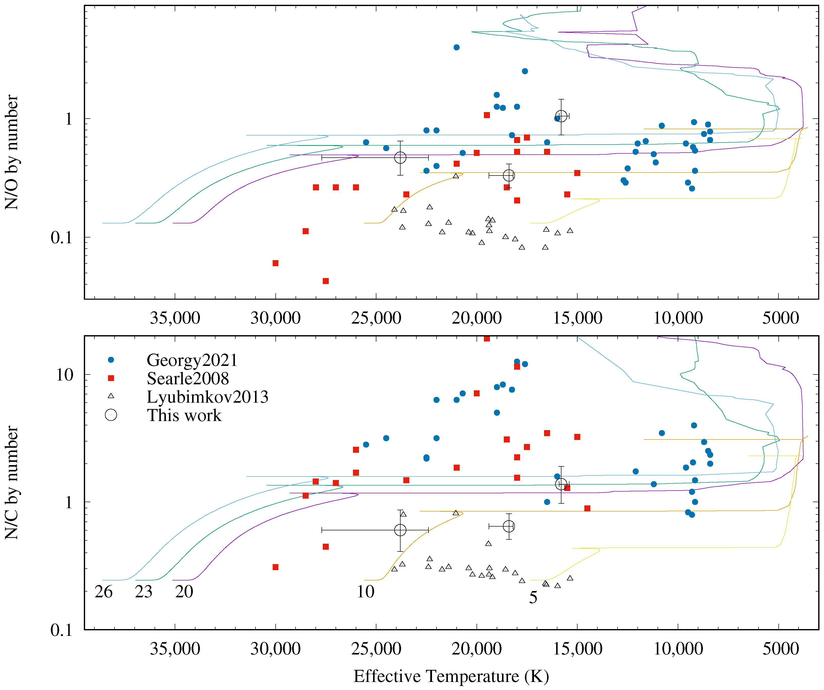
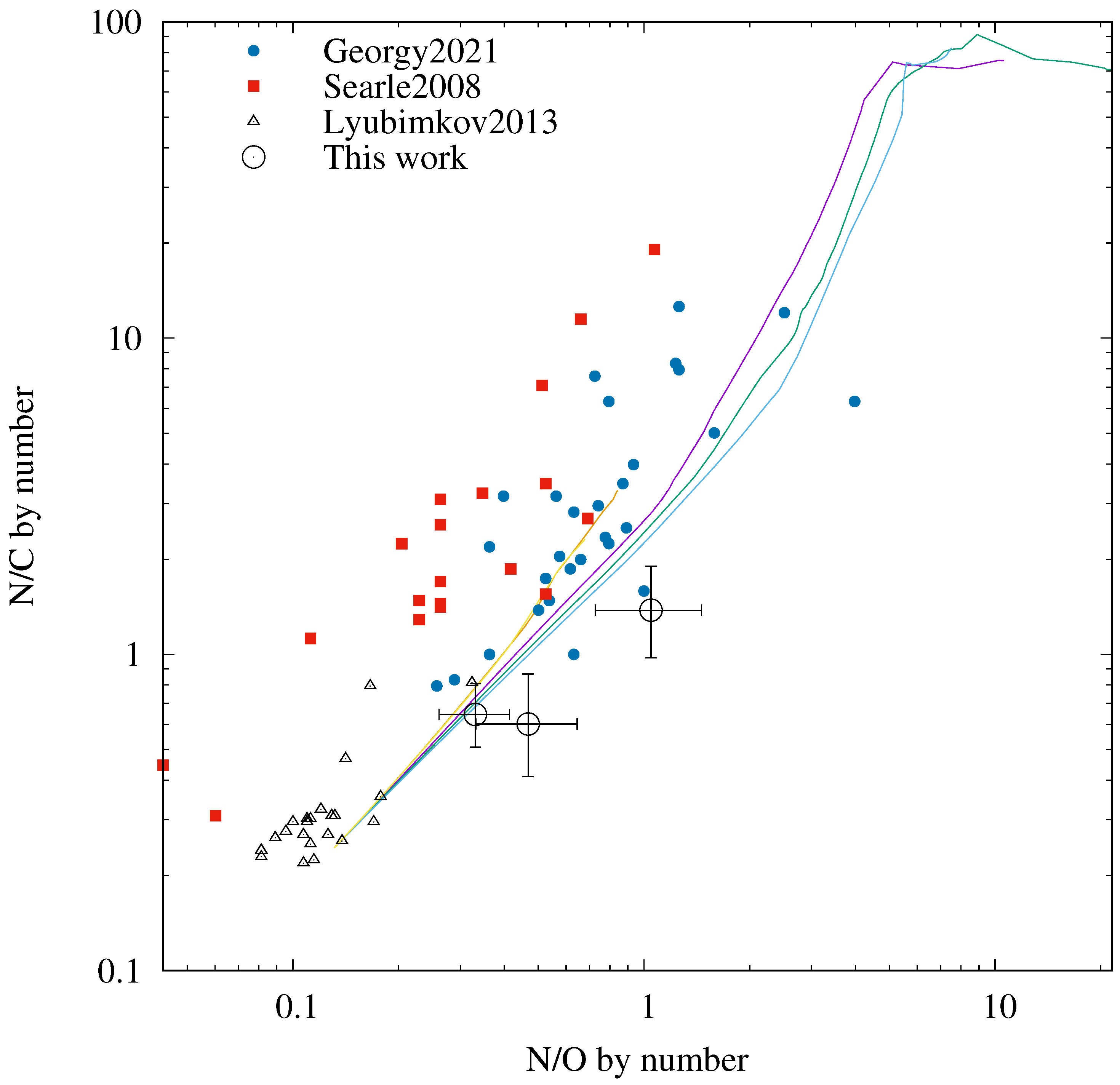
6.4. Surface Abundances
7. Conclusions
- A large sample of BSGs needs to be studied with homogenously modeled datasets of multi-epoch observations, with the aim of uncovering systematic deviations of surface abundance ratios from evolutionary models. Additionally, multi-epoch observations will allow us to place constraints on the current uncertainties observed in the radii of these objects and to identify changes in radii caused by radial pulsations.
- To frame the current studies for the needed M/M ratio for massive stars to evolve back towards the blue region of the HR diagram, such as the effect of stellar rotation, convective boundaries criteria, mixing length theories, overshooting that is adopted for the stellar interior, and evolutionary models, in terms of the CNO abundances. This will allow us to untackle the observed indetermination in the evolutionary stage of these objects with precise values for their CNO surface abundances and, in turn, will help to set the needed constraints to the current poorly established theoretical mass-loss recipes in the diverse evolutionary states and mass ranges.
- In addition, we emphasize that stellar pulsations play a key role in the analysis of BSGs, not only as a test to infer their evolutionary stage, as proposed in Saio et al. [15], but also as a mechanism that facilitates the mass loss in massive stars, as suggested in Kraus et al. [10] and theoretically confirmed in Yadav and Glatzel [72], affecting, therefore, their surface abundances. The systematic differences noticed when comparing evolutionary tracks with surface abundance measurements for BSGs (Figure 18) should be discussed, considering the effect of stellar pulsations over their evolution. Furthermore, short-term mass-loss variabilities should be contemplated in detailed evolutionary sequences, as they can act as an additional source for the discrepancies found with evolutionary models.
Author Contributions
Funding
Data Availability Statement
Acknowledgments
Conflicts of Interest
| 1 | IRAF is distributed by the National Optical Astronomy Observatory, which is operated by the Association of Universities for Research in Astronomy (AURA) under a cooperative agreement with the National Science Foundation. |
| 2 | https://xtgrid.astroserver.org/, (accessed on 20 August 2023). |
References
- Abbott, D.C. The return of mass and energy to the interstellar medium by winds from early-type stars. Astrophys. J. 1982, 263, 723–735. [Google Scholar] [CrossRef]
- Martins, F.; Palacios, A. A comparison of evolutionary tracks for single Galactic massive stars. Astron. Astrophys. 2013, 560, A16. [Google Scholar] [CrossRef]
- Agrawal, P.; Szécsi, D.; Stevenson, S.; Eldridge, J.J.; Hurley, J. Explaining the differences in massive star models from various simulations. Mon. Not. RAS 2022, 512, 5717–5725. [Google Scholar] [CrossRef]
- Yusof, N.; Hirschi, R.; Eggenberger, P.; Ekström, S.; Georgy, C.; Sibony, Y.; Crowther, P.A.; Meynet, G.; Kassim, H.A.; Harun, W.A.W.; et al. Grids of stellar models with rotation VII: Models from 0.8 to 300 M⊙ at supersolar metallicity (Z = 0.020). Mon. Not. RAS 2022, 511, 2814–2828. [Google Scholar] [CrossRef]
- Maeder, A.; Meynet, G. Evolution of massive stars with mass loss and rotation. New Astron. Rev. 2010, 54, 32–38. [Google Scholar] [CrossRef]
- Wagle, G.A.; Ray, A.; Dev, A.; Raghu, A. Type IIP Supernova Progenitors and Their Explodability. I. Convective Overshoot, Blue Loops, and Surface Composition. Astrophys. J. 2019, 886, 27. [Google Scholar] [CrossRef]
- Bowman, D.M.; Burssens, S.; Pedersen, M.G.; Johnston, C.; Aerts, C.; Buysschaert, B.; Michielsen, M.; Tkachenko, A.; Rogers, T.M.; Edelmann, P.V.F.; et al. Low-frequency gravity waves in blue supergiants revealed by high-precision space photometry. Nat. Astron. 2019, 3, 760–765. [Google Scholar] [CrossRef]
- Langer, N. Presupernova Evolution of Massive Single and Binary Stars. Annu. Rev. Astron Astrophys. 2012, 50, 107–164. [Google Scholar] [CrossRef]
- Glatzel, W. On the origin of strange modes and the mechanism of related instabilities. Mon. Not. RAS 1994, 271, 66. [Google Scholar] [CrossRef]
- Kraus, M.; Haucke, M.; Cidale, L.S.; Venero, R.O.J.; Nickeler, D.H.; Németh, P.; Niemczura, E.; Tomić, S.; Aret, A.; Kubát, J.; et al. Interplay between pulsations and mass loss in the blue supergiant 55 Cygnus = HD 198 478. Astron. Astrophys. 2015, 581, A75. [Google Scholar] [CrossRef]
- Haucke, M.; Cidale, L.S.; Venero, R.O.J.; Curé, M.; Kraus, M.; Kanaan, S.; Arcos, C. Wind properties of variable B supergiants. Evidence of pulsations connected with mass-loss episodes. Astron. Astrophys. 2018, 614, A91. [Google Scholar] [CrossRef]
- Aerts, C.; Lefever, K.; Baglin, A.; Degroote, P.; Oreiro, R.; Vučković, M.; Smolders, K.; Acke, B.; Verhoelst, T.; Desmet, M.; et al. Periodic mass-loss episodes due to an oscillation mode with variable amplitude in the hot supergiant HD 50064. Astron. Astrophys. 2010, 513, L11. [Google Scholar] [CrossRef]
- Saio, H.; Kuschnig, R.; Gautschy, A.; Cameron, C.; Walker, G.A.H.; Matthews, J.M.; Guenther, D.B.; Moffat, A.F.J.; Rucinski, S.M.; Sasselov, D.; et al. MOST Detects g- and p-Modes in the B Supergiant HD 163899 (B2 Ib/II). Astrophys. J. 2006, 650, 1111–1118. [Google Scholar] [CrossRef]
- Ostrowski, J.; Daszyńska-Daszkiewicz, J. Pulsations in B-type supergiants with masses M<20 M⊙ before and after core helium ignition. Mon. Not. RAS 2015, 447, 2378–2386. [Google Scholar] [CrossRef]
- Saio, H.; Georgy, C.; Meynet, G. Evolution of blue supergiants and α Cygni variables: Puzzling CNO surface abundances. Mon. Not. RAS 2013, 433, 1246–1257. [Google Scholar] [CrossRef]
- Németh, P.; Kawka, A.; Vennes, S. A selection of hot subluminous stars in the GALEX survey - II. Subdwarf atmospheric parameters. Mon. Not. RAS 2012, 427, 2180–2211. [Google Scholar] [CrossRef]
- Searle, S.C.; Prinja, R.K.; Massa, D.; Ryans, R. Quantitative studies of the optical and UV spectra of Galactic early B supergiants. I. Fundamental parameters. Astron. Astrophys. 2008, 481, 777–797. [Google Scholar] [CrossRef]
- Morel, T.; Marchenko, S.V.; Pati, A.K.; Kuppuswamy, K.; Carini, M.T.; Wood, E.; Zimmerman, R. Large-scale wind structures in OB supergiants: A search for rotationally modulated Hα variability. Mon. Not. RAS 2004, 351, 552–568. [Google Scholar] [CrossRef]
- Morel, T.; Hubrig, S.; Briquet, M. Nitrogen enrichment, boron depletion and magnetic fields in slowly-rotating B-type dwarfs. Astron. Astrophys. 2008, 481, 453–463. [Google Scholar] [CrossRef]
- Fossati, L.; Castro, N.; Morel, T.; Langer, N.; Briquet, M.; Carroll, T.A.; Hubrig, S.; Nieva, M.F.; Oskinova, L.M.; Przybilla, N.; et al. B fields in OB stars (BOB): On the detection of weak magnetic fields in the two early B-type stars β CMa and ϵ CMa. Possible lack of a “magnetic desert” in massive stars. Astron. Astrophys. 2015, 574, A20. [Google Scholar] [CrossRef]
- Lefever, K.; Puls, J.; Aerts, C. Statistical properties of a sample of periodically variable B-type supergiants. Evidence for opacity-driven gravity-mode oscillations. Astron. Astrophys. 2007, 463, 1093–1109. [Google Scholar] [CrossRef]
- Ekström, S.; Georgy, C.; Eggenberger, P.; Meynet, G.; Mowlavi, N.; Wyttenbach, A.; Granada, A.; Decressin, T.; Hirschi, R.; Frischknecht, U.; et al. Grids of stellar models with rotation. I. Models from 0.8 to 120 M⊙ at solar metallicity (Z = 0.014). Astron. Astrophys. 2012, 537, A146. [Google Scholar] [CrossRef]
- Ricker, G.R.; Winn, J.N.; Vanderspek, R.; Latham, D.W.; Bakos, G.Á.; Bean, J.L.; Berta-Thompson, Z.K.; Brown, T.M.; Buchhave, L.; Butler, N.R.; et al. Transiting Exoplanet Survey Satellite (TESS). In Space Telescopes and Instrumentation 2014: Optical, Infrared, and Millimeter Wave; Oschmann, J.M., Clampin, M., Fazio, G.G., MacEwen, H.A., Eds.; Society of Photo-Optical Instrumentation Engineers (SPIE) Conference Series; SPIE: Bellingham, WA, USA, 2014; Volume 9143, p. 914320. [Google Scholar] [CrossRef]
- Ricker, G.R.; Winn, J.N.; Vanderspek, R.; Latham, D.W.; Bakos, G.Á.; Bean, J.L.; Berta-Thompson, Z.K.; Brown, T.M.; Buchhave, L.; Butler, N.R.; et al. Transiting Exoplanet Survey Satellite (TESS). J. Astron. Telesc. Instruments Syst. 2015, 1, 014003. [Google Scholar] [CrossRef]
- Ginsburg, A.; Sipocz, B.M.; Brasseur, C.E.; Cowperthwaite, P.S.; Craig, M.W.; Deil, C.; Guillochon, J.; Guzman, G.; Liedtke, S.; Lian Lim, P.; et al. astroquery: An Astronomical Web-querying Package in Python. Astron. J. 2019, 157, 98. [Google Scholar] [CrossRef]
- Lightkurve Collaboration; Cardoso, J.V.d.M.; Hedges, C.; Gully-Santiago, M.; Saunders, N.; Cody, A.M.; Barclay, T.; Hall, O.; Sagear, S.; Turtelboom, E.; et al. Lightkurve: Kepler and TESS Time Series Analysis in Python; Astrophysics Source Code Library: College Park, MD, USA, 2018; Available online: https://arxiv.org/pdf/2111.14278.pdf (accessed on 16 March 2023).
- Garcia, S.; Van Reeth, T.; De Ridder, J.; Tkachenko, A.; IJspeert, L.; Aerts, C. Detection of period-spacing patterns due to the gravity modes of rotating dwarfs in the TESS southern continuous viewing zone. Astron. Astrophys. 2022, 662, A82. [Google Scholar] [CrossRef]
- Lenz, P.; Breger, M. Period04 User Guide. Commun. Asteroseismol. 2005, 146, 53–136. [Google Scholar] [CrossRef]
- Baran, A.S.; Koen, C. A Detection Threshold in the Amplitude Spectra Calculated from TESS Time-Series Data. Acta Astron. 2021, 71, 113–121. [Google Scholar] [CrossRef]
- Hillier, D.J.; Miller, D.L. The Treatment of Non-LTE Line Blanketing in Spherically Expanding Outflows. Astrophys. J. 1998, 496, 407–427. [Google Scholar] [CrossRef]
- Bouret, J.C.; Hillier, D.J.; Lanz, T.; Fullerton, A.W. Properties of Galactic early-type O-supergiants. A combined FUV-UV and optical analysis. Astron. Astrophys. 2012, 544, A67. [Google Scholar] [CrossRef]
- de Almeida, E.S.G.; Hugbart, M.; Domiciano de Souza, A.; Rivet, J.P.; Vakili, F.; Siciak, A.; Labeyrie, G.; Garde, O.; Matthews, N.; Lai, O.; et al. Combined spectroscopy and intensity interferometry to determine the distances of the blue supergiants P Cygni and Rigel. Mon. Not. RAS 2022, 515, 1–12. [Google Scholar] [CrossRef]
- Bouret, J.C.; Lanz, T.; Martins, F.; Marcolino, W.L.F.; Hillier, D.J.; Depagne, E.; Hubeny, I. Massive stars at low metallicity. Evolution and surface abundances of O dwarfs in the SMC. Astron. Astrophys. 2013, 555, A1. [Google Scholar] [CrossRef]
- Hillier, D.J.; Davidson, K.; Ishibashi, K.; Gull, T. On the Nature of the Central Source in η Carinae. Astrophys. J. 2001, 553, 837–860. [Google Scholar] [CrossRef]
- Eversberg, T.; Lépine, S.; Moffat, A.F.J. Outmoving Clumps in the Wind of the Hot O Supergiant ζ Puppis. Astrophys. J. 1998, 494, 799–805. [Google Scholar] [CrossRef]
- Bouret, J.C.; Lanz, T.; Hillier, D.J. Lower mass loss rates in O-type stars: Spectral signatures of dense clumps in the wind of two Galactic O4 stars. Astron. Astrophys. 2005, 438, 301–316. [Google Scholar] [CrossRef]
- Martins, F.; Marcolino, W.; Hillier, D.J.; Donati, J.F.; Bouret, J.C. Radial dependence of line profile variability in seven O9-B0.5 stars. Astron. Astrophys. 2015, 574, A142. [Google Scholar] [CrossRef]
- Sander, A.A.C. Recent advances in non-LTE stellar atmosphere models. In Proceedings of the The Lives and Death-Throes of Massive Stars; Eldridge, J.J., Bray, J.C., McClelland, L.A.S., Xiao, L., Eds.; Society of Photo-Optical Instrumentation Engineers (SPIE) Conference Series; ISPIE: Bellingham, WA, USA, 2017; Volume 329, pp. 215–222. Available online: https://www.cambridge.org/core/journals/proceedings-of-the-international-astronomical-union/article/recent-advances-in-nonlte-stellar-atmosphere-models/B993A4F409FCE7BACF9DAE43CCCF908B (accessed on 16 March 2023). [CrossRef]
- Martins, F.; Schaerer, D.; Hillier, D.J.; Meynadier, F.; Heydari-Malayeri, M.; Walborn, N.R. On stars with weak winds: The Galactic case. Astron. Astrophys. 2005, 441, 735–762. [Google Scholar] [CrossRef]
- Marcolino, W.L.F.; Bouret, J.C.; Martins, F.; Hillier, D.J.; Lanz, T.; Escolano, C. Analysis of Galactic late-type O dwarfs: More constraints on the weak wind problem. Astron. Astrophys. 2009, 498, 837–852. [Google Scholar] [CrossRef]
- de Almeida, E.S.G.; Marcolino, W.L.F.; Bouret, J.C.; Pereira, C.B. Probing the weak wind phenomenon in Galactic O-type giants. Astron. Astrophys. 2019, 628, A36. [Google Scholar] [CrossRef]
- Rivet, J.P.; Siciak, A.; de Almeida, E.S.G.; Vakili, F.; Domiciano de Souza, A.; Fouché, M.; Lai, O.; Vernet, D.; Kaiser, R.; Guerin, W. Intensity interferometry of P Cygni in the H α emission line: Towards distance calibration of LBV supergiant stars. Mon. Not. RAS 2020, 494, 218–227. [Google Scholar] [CrossRef]
- Hubeny, I.; Lanz, T. Non-LTE Line-blanketed Model Atmospheres of Hot Stars. I. Hybrid Complete Linearization/Accelerated Lambda Iteration Method. Astrophys. J. 1995, 439, 875. [Google Scholar] [CrossRef]
- Lanz, T.; Hubeny, I. A Grid of NLTE Line-blanketed Model Atmospheres of Early B-Type Stars. Astrophys. J. Suppl. 2007, 169, 83–104. [Google Scholar] [CrossRef]
- Hubeny, I.; Lanz, T. TLUSTY User’s Guide III: Operational Manual. arXiv 2017, arXiv:1706.01937. [Google Scholar] [CrossRef]
- Lin, J.; Wu, C.; Wang, X.; Németh, P.; Xiong, H.; Wu, T.; Filippenko, A.V.; Cai, Y.; Brink, T.G.; Yan, S.; et al. An 18.9 min blue large-amplitude pulsator crossing the `Hertzsprung gap’ of hot subdwarfs. Nat. Astron. 2023, 7, 223–233. [Google Scholar] [CrossRef]
- Lei, Z.; He, R.; Nemeth, P.; Zou, X.; Xiao, H.; Yang, Y.; Zhao, J. Mass distribution for single-lined hot subdwarf stars in LAMOST. arXiv 2023, arXiv:2306.15342. [Google Scholar] [CrossRef]
- Németh, P.; Vos, J.; Molina, F.; Bastian, A. The first heavy-metal hot subdwarf composite binary SB 744. Astron. Astrophys. 2021, 653, A3. [Google Scholar] [CrossRef]
- Luo, Y.; Németh, P.; Li, Q. Hot Subdwarf Stars Identified in Gaia DR2 with Spectra of LAMOST DR6 and DR7. II.Kinematics. Astrophys. J. 2020, 898, 64. [Google Scholar] [CrossRef]
- Wang, K.; Németh, P.; Luo, Y.; Chen, X.; Jiang, Q.; Cao, X. Extremely Low-mass White Dwarf Stars Observed in Gaia DR2 and LAMOST DR8. Astrophys. J. 2022, 936, 5. [Google Scholar] [CrossRef]
- Vennes, S.; Nemeth, P.; Kawka, A.; Thorstensen, J.R.; Khalack, V.; Ferrario, L.; Alper, E.H. An unusual white dwarf star may be a surviving remnant of a subluminous Type Ia supernova. Science 2017, 357, 680–683. [Google Scholar] [CrossRef]
- Asplund, M.; Grevesse, N.; Sauval, A.J.; Scott, P. The Chemical Composition of the Sun. Annu. Rev. Astron Astrophys. 2009, 47, 481–522. [Google Scholar] [CrossRef]
- Vink, J.S.; de Koter, A.; Lamers, H.J.G.L.M. Mass-loss predictions for O and B stars as a function of metallicity. Astron. Astrophys. 2001, 369, 574–588. [Google Scholar] [CrossRef]
- de Jager, C.; Nieuwenhuijzen, H.; van der Hucht, K.A. Mass loss rates in the Hertzsprung-Russell diagram. Astron. Astrophys. Suppl. 1988, 72, 259–289. [Google Scholar]
- Maeder, A.; Meynet, G. Stellar evolution with rotation. VI. The Eddington and Omega -limits, the rotational mass loss for OB and LBV stars. Astron. Astrophys. 2000, 361, 159–166. [Google Scholar] [CrossRef]
- Capitanio, L.; Lallement, R.; Vergely, J.L.; Elyajouri, M.; Monreal-Ibero, A. Three-dimensional mapping of the local interstellar medium with composite data. Astron. Astrophys. 2017, 606, A65. [Google Scholar] [CrossRef]
- Cardelli, J.A.; Clayton, G.C.; Mathis, J.S. The Relationship between Infrared, Optical, and Ultraviolet Extinction. Astrophys. J. 1989, 345, 245. [Google Scholar] [CrossRef]
- Fitzpatrick, E.L.; Massa, D. An Analysis of the Shapes of Ultraviolet Extinction Curves. I. The 2175 Angstrom Bump. Astrophys. J. 1986, 307, 286. [Google Scholar] [CrossRef]
- Fitzpatrick, E.L.; Massa, D. An Analysis of the Shapes of Ultraviolet Extinction Curves. II. The Far-UV Extinction. Astrophys. J. 1988, 328, 734. [Google Scholar] [CrossRef]
- Krtička, J.; Feldmeier, A. Stochastic light variations in hot stars from wind instability: Finding photometric signatures and testing against the TESS data. Astron. Astrophys. 2021, 648, A79. [Google Scholar] [CrossRef]
- Saio, H. Linear analyses for the stability of radial and non-radial oscillations of massive stars. Mon. Not. RAS 2011, 412, 1814–1822. [Google Scholar] [CrossRef]
- Zickgraf, F.J.; Kovacs, J.; Wolf, B.; Stahl, O.; Kaufer, A.; Appenzeller, I. R4 in the Small Magellanic Cloud: A spectroscopic binary with a B[e]/LBV-type component. Astron. Astrophys. 1996, 309, 505–514. [Google Scholar]
- Wu, S.; Everson, R.W.; Schneider, F.R.N.; Podsiadlowski, P.; Ramirez-Ruiz, E. The Art of Modeling Stellar Mergers and the Case of the B[e] Supergiant R4 in the Small Magellanic Cloud. Astrophys. J. 2020, 901, 44. [Google Scholar] [CrossRef]
- van Leeuwen, F. Validation of the new Hipparcos reduction. Astron. Astrophys. 2007, 474, 653–664. [Google Scholar] [CrossRef]
- Burssens, S.; Simón-Díaz, S.; Bowman, D.M.; Holgado, G.; Michielsen, M.; de Burgos, A.; Castro, N.; Barbá, R.H.; Aerts, C. Variability of OB stars from TESS southern Sectors 1-13 and high-resolution IACOB and OWN spectroscopy. Astron. Astrophys. 2020, 639, A81. [Google Scholar] [CrossRef]
- Nieva, M.F.; Przybilla, N. C II Abundances in Early-Type Stars: Solution to a Notorious Non-LTE Problem. Astrophys. J. Lett. 2006, 639, L39–L42. [Google Scholar] [CrossRef]
- Georgy, C.; Saio, H.; Meynet, G. Blue supergiants as tests for stellar physics. Astron. Astrophys. 2021, 650, A128. [Google Scholar] [CrossRef]
- Lyubimkov, L.S.; Lambert, D.L.; Poklad, D.B.; Rachkovskaya, T.M.; Rostopchin, S.I. Carbon, nitrogen and oxygen abundances in atmospheres of the 5–11 M⊙ B-type main-sequence stars. Mon. Not. RAS 2013, 428, 3497–3508. [Google Scholar] [CrossRef]
- Krtička, J.; Kubát, J.; Krtičková, I. New mass-loss rates of B supergiants from global wind models. Astron. Astrophys. 2021, 647, A28. [Google Scholar] [CrossRef]
- Martins, F.; Hervé, A.; Bouret, J.C.; Marcolino, W.; Wade, G.A.; Neiner, C.; Alecian, E.; Grunhut, J.; Petit, V. The MiMeS survey of magnetism in massive stars: CNO surface abundances of Galactic O stars. Astron. Astrophys. 2015, 575, A34. [Google Scholar] [CrossRef]
- Davies, B.; Kudritzki, R.P.; Plez, B.; Trager, S.; Lançon, A.; Gazak, Z.; Bergemann, M.; Evans, C.; Chiavassa, A. The Temperatures of Red Supergiants. Astrophys. J. 2013, 767, 3. [Google Scholar] [CrossRef]
- Yadav, A.P.; Glatzel, W. Stability analysis, non-linear pulsations and mass loss of models for 55 Cygni (HD 198478). Mon. Not. RAS 2016, 457, 4330–4339. [Google Scholar] [CrossRef]
- Zsargó, J.; Fierro-Santillán, C.R.; Klapp, J.; Arrieta, A.; Arias, L.; Valencia, J.M.; Sigalotti, L.D.G.; Hareter, M.; Puebla, R.E. Creating and using large grids of precalculated model atmospheres for a rapid analysis of stellar spectra. Astron. Astrophys. 2020, 643, A88. [Google Scholar] [CrossRef]
- Gregorio, A.; Stalio, R.; Broadfoot, L.; Castelli, F.; Hack, M.; Holberg, J. UVSTAR observations of Adara (epsilon CMa): 575-1250 Å. Astron. Astrophys. 2002, 383, 881–891. [Google Scholar] [CrossRef]


| Parameter | HD 42087 | HD 52089 | HD 58350 |
|---|---|---|---|
| [K] | 16,500 ± 1000 | 23,000 ± 1000 | 15,500 ± 700 |
| [cgs] | 2.45 ± 0.10 | 3.00 ± 0.10 | 2.00 ± 0.10 |
| [] | 5.31 ± 0.43 | 4.49 ± 0.05 | 5.18 ± 0.32 |
| [] | 55 | 11 | 54 |
| [km s] | 80 | 10 | 40 |
| [ yr] | (5.7 ± 0.5) | (2.0 ± 0.6) | (1.4 ± 0.2) |
| [km s] | 700 ± 70 | 900 ± 270 | 200 ± 30 |
| 2.0 | 1.0 | 3.0 |
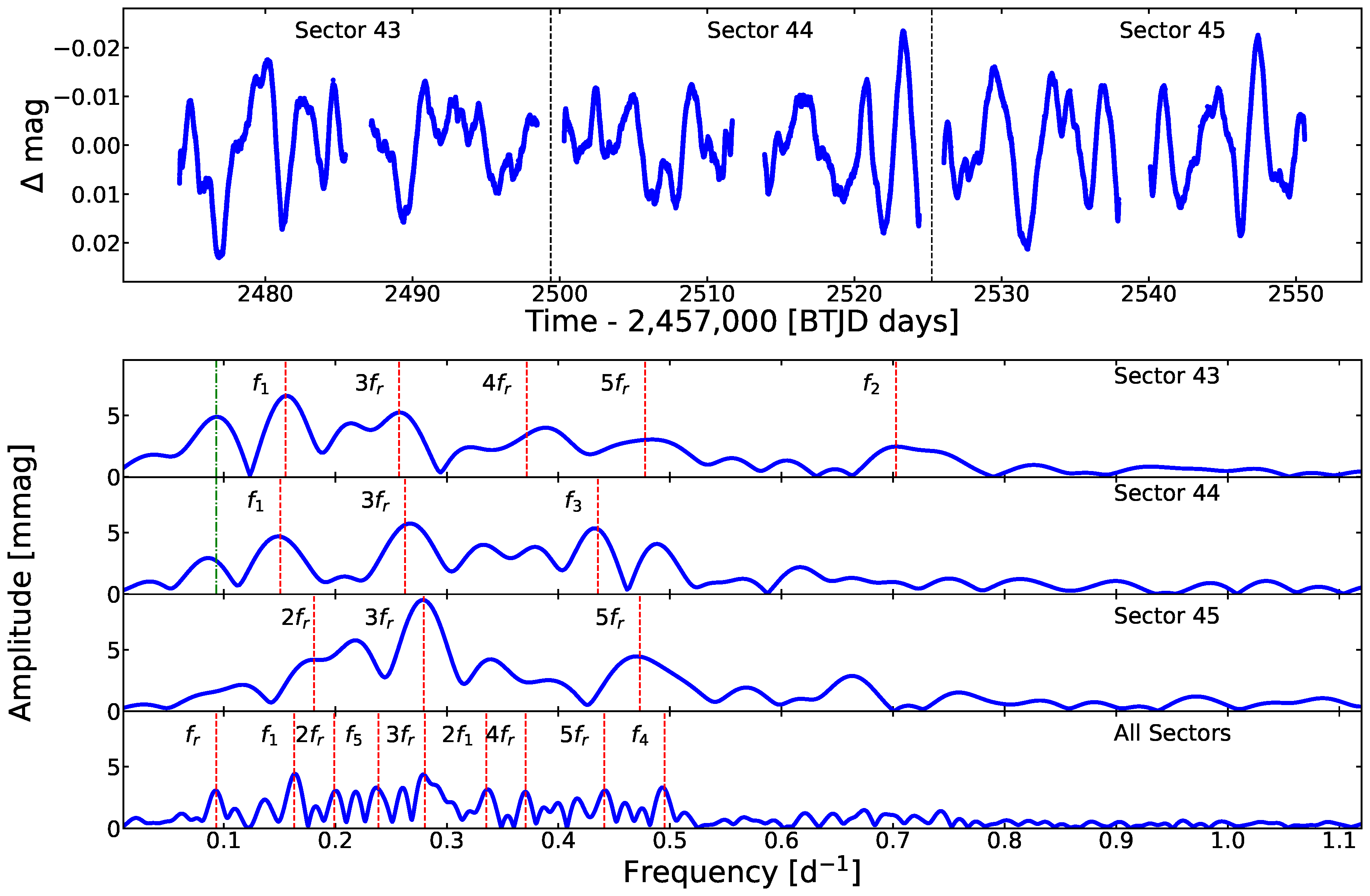
| Sector | Frequency [] | 3 [] | Amplitude [mmag] | 3 [mmag] | S/N | Id |
|---|---|---|---|---|---|---|
| 0.15543 | 0.00044 | 7.7615 | 0.15 | 10.65 | ||
| 0.25729 | 0.00063 | 5.7467 | 0.14 | 8.41 | ||
| 43 | 0.47759 | 0.00064 | 4.7663 | 0.13 | 7.79 | |
| 0.37169 | 0.00090 | 3.5347 | 0.13 | 5.45 | ||
| 0.70257 | 0.00037 | 2.9734 | 0.14 | 5.41 | ||
| 0.26268 | 0.00068 | 5.5317 | 0.16 | 7.68 | ||
| 44 | 0.15072 | 0.00082 | 5.2203 | 0.17 | 6.75 | |
| 0.43536 | 0.00090 | 4.9832 | 0.19 | 7.45 | ||
| 0.27928 | 0.00009 | 9.2074 | 0.10 | 10.65 | ||
| 45 | 0.18110 | 0.00059 | 5.0188 | 0.13 | 5.57 | |
| 0.47295 | 0.00159 | 4.0068 | 0.21 | 5.07 | ||
| 0.28022 | 0.00019 | 4.4715 | 0.12 | 8.48 | ||
| 0.16305 | 0.00021 | 3.9728 | 0.11 | 7.05 | ||
| 0.49515 | 0.00022 | 3.4982 | 0.11 | 7.44 | ||
| 0.23874 | 0.00027 | 3.2680 | 0.11 | 6.04 | ||
| All | 0.44102 | 0.00023 | 3.2321 | 0.10 | 6.67 | |
| 0.33531 | 0.00030 | 2.9450 | 0.11 | 5.74 | ||
| 0.19899 | 0.00029 | 2.8086 | 0.10 | 5.07 | ||
| 0.37073 | 0.00033 | 2.6635 | 0.10 | 5.29 | ||
| 0.09321 | 0.00032 | 2.4597 | 0.12 | 4.20 |
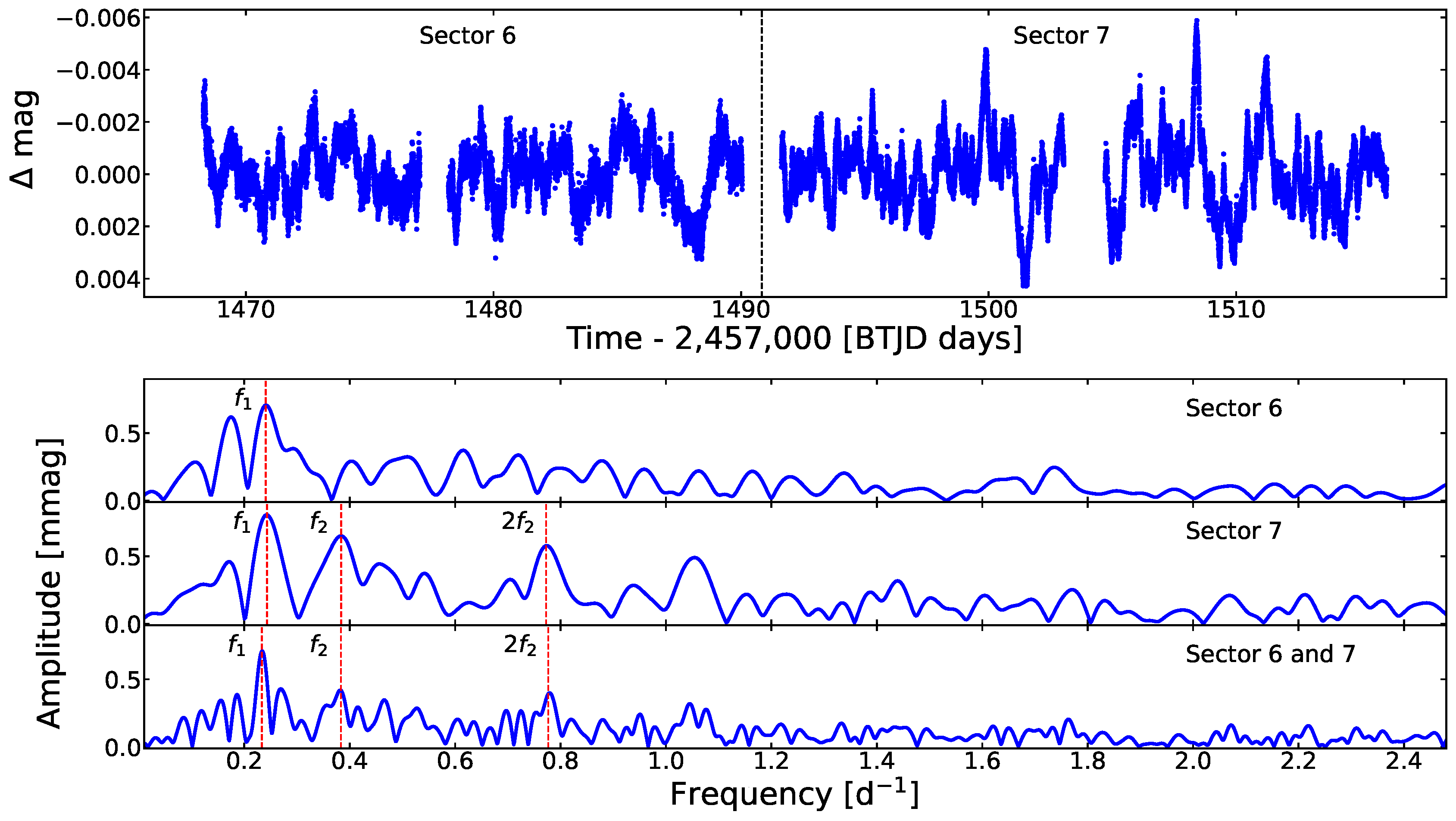
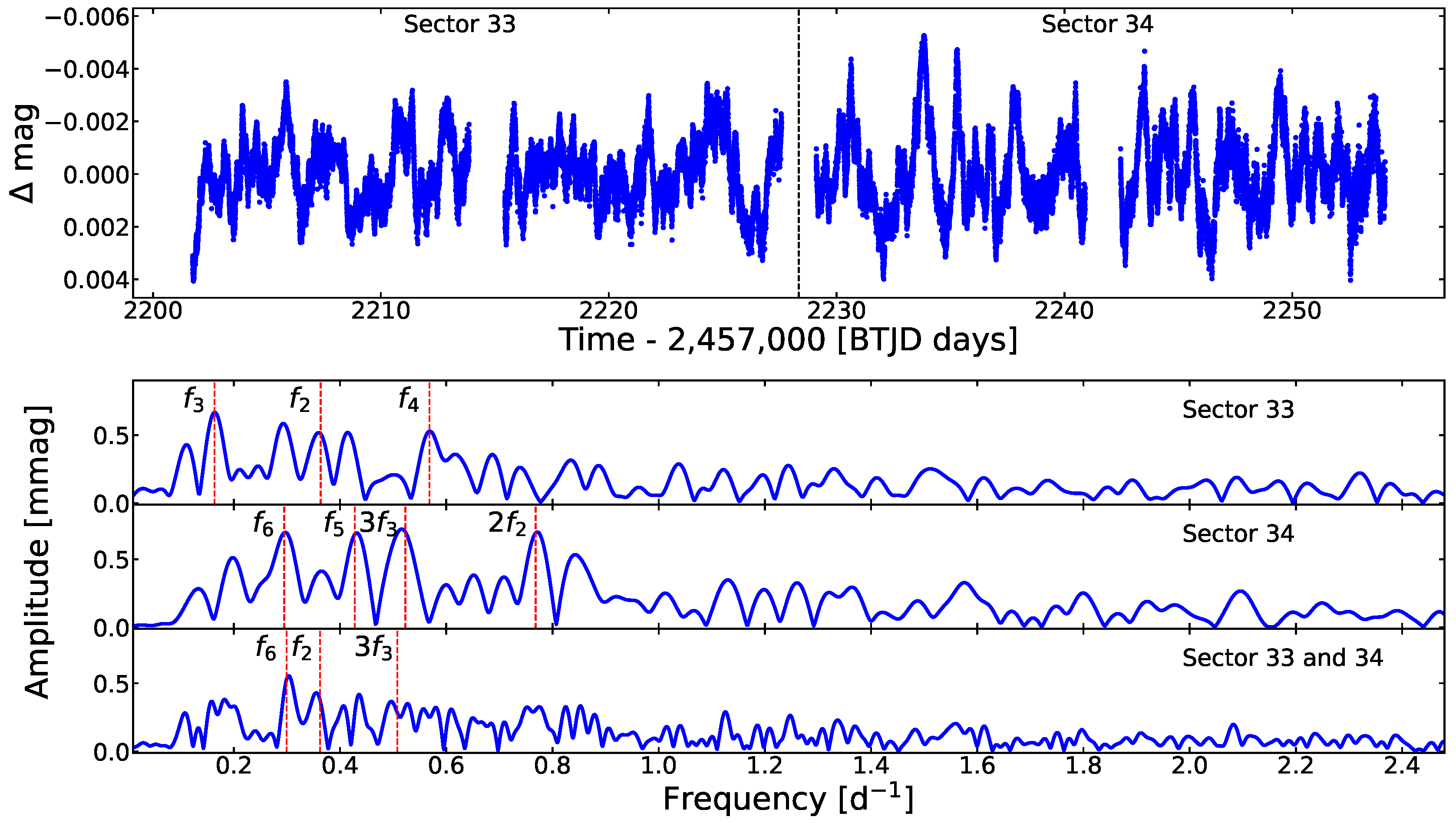
| Sector | Frequency [] | 3 [] | Amplitude [mmag] | 3 [mmag] | S/N | Id |
|---|---|---|---|---|---|---|
| 6 | 0.24083 | 0.00115 | 0.7830 | 0.05 | 6.15 | |
| 0.24316 | 0.01540 | 0.8982 | 0.47 | 6.14 | ||
| 7 | 0.38381 | 0.00192 | 0.7286 | 0.05 | 5.15 | |
| 0.77252 | 0.00051 | 0.5888 | 0.02 | 4.37 | ||
| 0.23321 | 0.00072 | 0.7736 | 0.07 | 7.28 | ||
| 6 & 7 | 0.38342 | 0.02775 | 0.4930 | 0.17 | 4.79 | |
| 0.77679 | 0.00073 | 0.4769 | 0.04 | 4.83 | ||
| 0.16358 | 0.00070 | 0.7716 | 0.02 | 6.868 | ||
| 33 | 0.36366 | 0.00089 | 0.5784 | 0.02 | 5.42 | |
| 0.56843 | 0.00089 | 0.5083 | 0.02 | 4.72 | ||
| 0.42781 | 0.00107 | 0.7556 | 0.03 | 4.98 | ||
| 34 | 0.52280 | 0.00128 | 0.7113 | 0.03 | 4.74 | |
| 0.76818 | 0.00127 | 0.7038 | 0.03 | 4.75 | ||
| 0.29483 | 0.00147 | 0.6389 | 0.03 | 4.35 | ||
| 0.29937 | 0.00167 | 0.6627 | 0.12 | 5.01 | ||
| 33 & 34 | 0.36220 | 0.00331 | 0.5806 | 0.34 | 4.39 | |
| 0.50772 | 0.00158 | 0.4714 | 0.09 | 4.09 |
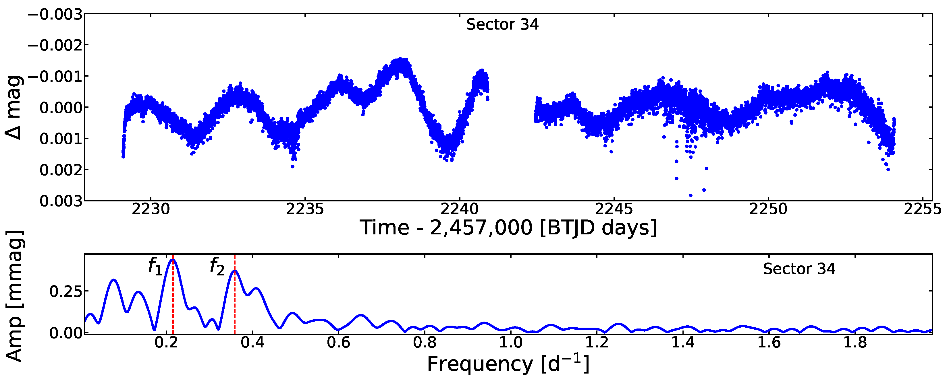
| Sector | Frequency [] | 3 [] | Amplitude [mmag] | 3 [mmag] | S/N | Id |
|---|---|---|---|---|---|---|
| 34 | 0.21533 | 0.00069 | 0.4392 | 0.01 | 8.54 | |
| 0.35927 | 0.00088 | 0.3339 | 0.01 | 7.07 |
| Ion | Full-Levels | Super-Levels | b-b Transitions |
|---|---|---|---|
| H i | 30 | 30 | 435 |
| He i | 69 | 69 | 905 |
| He ii | 30 | 30 | 435 |
| C ii | 322 | 92 | 7742 |
| C iii | 243 | 99 | 5528 |
| C iv | 64 | 64 | 1446 |
| N ii | 105 | 59 | 898 |
| N iii | 287 | 57 | 6223 |
| N iv | 70 | 44 | 440 |
| N v | 49 | 41 | 519 |
| O ii | 274 | 155 | 5880 |
| O iii | 104 | 36 | 761 |
| O iv | 64 | 30 | 359 |
| O v | 56 | 32 | 314 |
| Ne ii | 48 | 14 | 328 |
| Ne iii | 71 | 23 | 460 |
| Ne iv | 52 | 17 | 315 |
| Mg ii | 44 | 36 | 348 |
| Si ii | 53 | 27 | 278 |
| Si iii | 90 | 51 | 640 |
| Si iv | 66 | 66 | 1090 |
| S iii | 78 | 39 | 520 |
| S iv | 108 | 40 | 958 |
| S v | 144 | 37 | 1673 |
| Fe ii | 295 | 24 | 2135 |
| Fe iii | 607 | 65 | 6670 |
| Fe iv | 1000 | 100 | 37,899 |
| Fe v | 1000 | 139 | 37,737 |
| Fe vi | 1000 | 59 | 36,431 |
| Ni ii | 158 | 27 | 1668 |
| Ni iii | 150 | 24 | 1345 |
| Ni iv | 200 | 36 | 2337 |
| Ni v | 183 | 46 | 1524 |
| Ni vi | 182 | 40 | 1895 |
| Parameter | HD 42087 | HD 52089 | HD 58350 | |||
|---|---|---|---|---|---|---|
| (K) | ||||||
| 73.4 ± 8.0 | 38.4 ± 5.0 | 51.5 ± 5.0 | ||||
| x10 | x10 | x12 | ||||
| ( yr) | (1.9 ± 0.2) | (6.2 ± 2.0) | ||||
| x700 | x900 | x230 | ||||
| x2 | x1 | x3 | ||||
| () | ||||||
| () | 24.3 | 11.1 | 9.5 | |||
| () | x55 | x11 | x54 | |||
| 4.1 | 3.5 | 4.2 | ||||
| Mean atomic | 1.4490 | 1.5097 | 1.5095 | |||
| mass (a.m.u.) | ||||||
| Distance () | 2470 | 124 | 608 | |||
| E() () | 0.4 | 0.005 | 0.03 | |||
| Element | mass fr. | mass fr. | mass fr. | |||
| Hydrogen | 12 | 5.89 | 12 | 5.52 | 12 | 5.52 |
| Helium | x11.23 | 4.01 | x11.30 | 4.41 | x11.31 | 4.41 |
| Carbon | 8.31 | 1.37 | 8.19 | 1.04 | 8.07 | 7.75 |
| Nitrogen | 8.12 | 1.09 | 7.97 | 7.25 | 8.21 | 1.25 |
| Oxygen | 8.60 | 3.75 | 8.30 | 1.78 | 8.19 | 1.38 |
| [N/C] | [N/O] | [N/C] | [N/O] | [N/C] | [N/O] | |
| Abundance ratios | 0.41 | 0.38 | 0.38 | 0.53 | 0.74 | 0.88 |
Disclaimer/Publisher’s Note: The statements, opinions and data contained in all publications are solely those of the individual author(s) and contributor(s) and not of MDPI and/or the editor(s). MDPI and/or the editor(s) disclaim responsibility for any injury to people or property resulting from any ideas, methods, instructions or products referred to in the content. |
© 2023 by the authors. Licensee MDPI, Basel, Switzerland. This article is an open access article distributed under the terms and conditions of the Creative Commons Attribution (CC BY) license (https://creativecommons.org/licenses/by/4.0/).
Share and Cite
Sánchez Arias, J.P.; Németh, P.; de Almeida, E.S.d.G.; Ruiz Diaz, M.A.; Kraus, M.; Haucke, M. Unveiling the Evolutionary State of Three B Supergiant Stars: PU Gem, ϵ CMa, and η CMa. Galaxies 2023, 11, 93. https://doi.org/10.3390/galaxies11050093
Sánchez Arias JP, Németh P, de Almeida ESdG, Ruiz Diaz MA, Kraus M, Haucke M. Unveiling the Evolutionary State of Three B Supergiant Stars: PU Gem, ϵ CMa, and η CMa. Galaxies. 2023; 11(5):93. https://doi.org/10.3390/galaxies11050093
Chicago/Turabian StyleSánchez Arias, Julieta Paz, Péter Németh, Elisson Saldanha da Gama de Almeida, Matias Agustin Ruiz Diaz, Michaela Kraus, and Maximiliano Haucke. 2023. "Unveiling the Evolutionary State of Three B Supergiant Stars: PU Gem, ϵ CMa, and η CMa" Galaxies 11, no. 5: 93. https://doi.org/10.3390/galaxies11050093