
Introduction to Electroweak Baryogenesis

Instituto de Física, Pontificia Universidad Católica de Valparaíso, Av. Brasil 2950, Valparaíso 2340000, Chile
Galaxies 2022, 10(6), 116; https://doi.org/10.3390/galaxies10060116
Submission received: 14 November 2022
/
Accepted: 9 December 2022
/
Published: 12 December 2022
(This article belongs to the Special Issue Physical Processes in the Early Universe: Primordial Black Holes, Dark Matter, Baryon Asymmetry and All That)
Abstract
:We present a pedagogical introduction to the electroweak baryogenesis. The review focuses principally on the sphaleron and baryon number (non)-conservation or chiral anomaly. All results are derived with details for a self-contained reading.
1. Introduction
One of the very important aspects of the history of our universe is the missing antiparticles. The universe is composed essentially of matter and the rare particles of antimatter observed are not from the early time of our universe but are produced in some interactions, such as collisions in the atmosphere, with cosmic rays. The field that is trying to discover the history of these disappeared primordial antiparticles is known as baryogenesis. Many models have been constructed but while a large number are not falsifiable, at least with the current experiments, some have attracted more attention because they could produce a testable signature with gravitational waves. In particular, LISA (Laser Interferometer Space Antenna) could observe [1] a stochastic gravitational wave signal produced by an electroweak phase transition in the early universe, which is a central mechanism in the electroweak baryogenesis (EWBG). Therefore, EWBG and some other falsifiable models will be central in future research topics. For that reason, we believe that this review could be an introduction for students and young researchers who are not familiar with the field. This review is not a summary of the state-of-the-art in the area but more as lecture notes with great detail provided in the calculations. We should mention a few of the very interesting reviews covering many of the aspects mentioned in this review and more [2,3,4,5,6]. We hope that this review could be complementary for a non-expert audience.
In the first section of this review, we will introduce a brief history of the baryogenesis up to the Sakharov conditions, which are necessary but not sufficient conditions for any model of baryogenesis. In a second section, we will summarise our current knowledge of the baryon/antibaryon asymmetry from CMB (cosmic microwave background) and BBN (Big Bang nucleosynthesis) observations. In the third section, we will introduce the sphaleron process—which is central in the EWBG—via a toy model in dimensions and its relation to baryon number conservation. Finally, we will summarize the EWBG mechanism.
2. Sakharov Conditions
Before mentioning the three necessary conditions for any viable model of baryogenesis, it is important to summarise the current knowledge at the time of Andrei Sakharov.
The story starts with Paul Dirac, who proposed, with the help of the equation bearing his name, the existence of a sea of negative energy states. After some debates, in particular with Robert Oppenheimer and Hermann Weyl, Dirac interpreted this solution as describing a new particle with the same characteristics as the electron but with positive charge, an anti-electron which has been discovered and renamed by Carl Anderson in 1932 as a positron. The antiparticles were born. Since then, physicists have tried to observe their abundance, because according to the Dirac equation, there is no reason for an excess of matter over anti-matter. But if antimatter was equally present in the universe, we would see it. Indeed, if the Universe was half filled with anti-nucleons, we would have anti-galaxies, anti-stars which should produce via anti-star nucleosynthesis the heavy elements of anti-matter, but nothing has been observed, such as, e.g., an important component of antiprotons in the cosmic rays produced by anti-supernovas.
We could therefore easily imagine that matter and antimatter form large domains which are separated by voids. If that hypothesis was totally legitimate in the early studies, it has been totally ruled out by CMB observations 1. Indeed, any structures of antimatter would deform the CMB spectrum. Clearly, primary antimatter does not exist, only secondary antimatter particles exist, which are created from the collision of cosmic rays (protons) with the atmosphere or radioactive decay such as or decays.
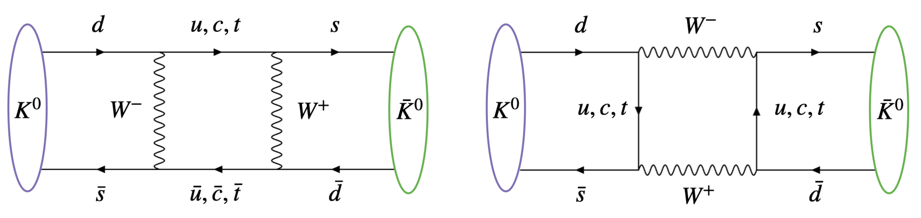
A first step towards an understanding of the difference between matter and antimatter was discovered in 1950. Indeed, P-symmetry is violated in weak interactions, the symmetry between left and right-handed particles. In this context, CP symmetry was postulated by Lev Landau in 1957 to restore order. For that, C-symmetry should also be violated, which was confirmed in various experiments. This new symmetry (CP) would not make any difference between matter and antimatter. Any left (right)-handed particle can be exchanged with a right (left)-handed antiparticle. To differentiate them, (CP) symmetry should be violated, which was discovered in 1964 by observing kaon decay, in particular , which is composed of a down quark and a strange antiquark, and , its antiparticle. It was discovered that transforms into which again transforms into . This is the phenomenon of oscillation, first studied in 1954 by Murray Gell-Mann and Abraham Pais (see Figure 1).
The mixing could be described by a state,
where because of CPT symmetry. We are working on the basis of
The operation of CP transforms particles into antiparticles and therefore , where is an irrelevant phase. Using theses relations, we can conclude that CP symmetry would imply , indeed,
where, in the last expression, we have used our assumption of CP invariance, . Under this assumption, the eigenstates of our Hamiltonian (1) become
However, in nature, two neutral kaons are known, which are distinguished by their lifetimes. A long-lived kaon which decays into three pions and a short lived one which decays into two pions. They should naturally be identified as the two eigenstates and . However, analysing a beam of kaons at a distance at which all short-lived ones should have decayed, and therefore only long-lived ones should exist, i.e., particles decaying into three pions, it was shown in 1964 that some particles were decaying into two pions. Concluding that both eigenstates could decay into two pions implies a CP-violation via states
where measures the deviation to exact CP-symmetry with [7]. Violation of CP-symmetry is a key element for baryogenesis.
In this context, Sakharov reached the conclusion that the problem of baryon asymmetry needed a dynamical solution with three conditions:
- Baryon number violating process;
- C-Symmetry and CP-symmetry violations;
- Departure from thermal equilibrium.
2.1. Baryon Number Violating Process
Let us first remember that the baryon number is defined as , while and are the number of quarks and antiquarks. It seems obvious that, if after inflation and all processes conserve B, we would never create the baryon asymmetry. So, we need processes such as , where and , which implies that in this process, we have . We will see that such a mechanism exists, and it is caused by the sphaleron.
2.2. C-symmetry and CP-Symmetry Violations
As we have seen in the previous section, we need processes that discriminate between baryons and antibaryons otherwise the process (for which ) would be as likely as , which implies that no net baryon number would be generated. More formally, we need to violate processes in which the baryon number is changed into its negative. We have and , while is here to be understood as an operator for which we have , with the density operator solution of the Liouville equation
If C and are exact symmetries, they commute with the Hamiltonian, and therefore with ,
which implies , and similarly with symmetry.
2.3. Departure from Thermal Equilibrium
If we have thermal equilibrium, the process is compensated by and therefore the total baryon number remains zero. This third condition can also be proved more formally. Because we do not have time evolution, we will not use the Liouville equation but instead the CPT theorem which states that CPT is an exact symmetry. We have because in equilibrium time inversion does not change the sign of B. If the system is in equilibrium, the density matrix is thermal which implies and therefore . We need a process out of equilibrium.
We conclude this section with the Sakharov conditions which are a guiding rail for viable models of baryogenesis. We need to be sure that all three conditions are met and also that the asymmetry is sufficient to explain our universe.
3. Baryon Asymmetry from Observations
If in the early universe for antibaryons we had baryons, our problem would be solved. This very precise statistics comes from observations such as BBN and CMB. In order to quantify the problem, we need to know the difference between baryons and antibaryons. For that, it is customary to define , where and are the number of baryons and antibaryons, respectively, and s is the total entropy density. This expression is convenient because is conserved. Indeed, if , we have 2 but, using the equation of conservation, , we obtain which implies that, for non-degenerate matter or when it is neither created nor destroyed ), the entropy is conserved 3. We conclude that because and scale as , is conserved. Another variable is often defined in the literature, , which is, during most of the history of the universe, conserved, except at the early times because the particles which were in equilibrium were annihilated to produce photons but no baryons and therefore decreased. However, we can consider as a constant parameter after this epoch and therefore during BBN and CMB until today.
We know from observations that today antibaryons are very negligible, so . Additionally, baryons are, at our epoch, non-relativistic, so we can approximate where is the mass of the baryons. Considering that most of them are protons, we have . Therefore, we have
and therefore or where we used (see Appendix A). If we take a better estimate of the baryon mass [8], we obtain , which can be easily converted into ,
where the last expression is derived in more detail in the Appendix B.
The BBN and the CMB are very sensitive to the amount of baryons in the universe. They constrain [9] or [8], which imply
Both BBN and CMB produce very similar results which indicates a very strong confidence in our knowledge of the baryon asymmetry of the universe (BAU). This asymmetry should be produced before the annihilation epoch. In the very early universe, processes are in thermal equilibrium but once the energy of the photons decreases enough, we cannot maintain the reverse process, which implies an annihilation between matter and antimatter. Therefore, we need an excess of matter such that to produce our current universe. It would be simple to imagine that it is part of the initial conditions of our Uuniverse and invoke some string landscape argument; we happen to live in a universe with . Unfortunately, inflation and sphaleron would washout any initial asymmetry; for these reasons, we need a dynamical process of baryogenesis.
4. Sphaleron Process
In the Standard Model (SM) of particle physics and in particular in electroweak theory, we have four global symmetries related to the conservation of leptonic numbers and baryonic numbers; for electron and electron neutrino, for muon and muon neutrino, for tau and tau neutrino and finally B for baryons. In the SM, B and are not conserved but is conserved. That means that we could have processes involving three leptons and three baryons or equivalently nine quarks, in which is conserved but B and L change. For example,
In this process, we have and and and . We have antimatter producing matter by violating the conservation of B and L but keeping constant. We will see that this process exists in the SM and fortunately is active only at high energies, such as in the early universe; otherwise, the proton (the lightest particle with non-zero baryon number) would be unstable via the antisphaleron process.
4.1. Complex Field Toy Model
As a starting point, let us consider a simple model in dimensions:
which gives
A static solution is
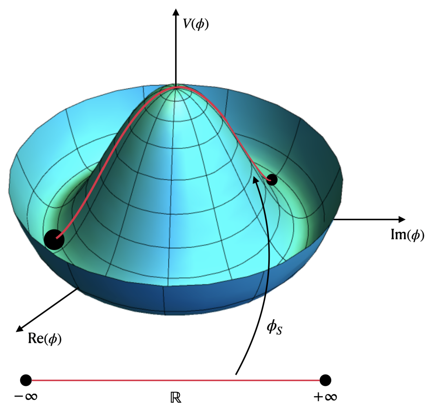
which is similar to the kink/antikink solution but with a factor , because the field is complex which makes it unstable, contrary to the soliton. Indeed, from Figure 2 we see that the additional dimension (complex solution) makes the solution unstable under small perturbations. This is the simplest sphaleron configuration.
4.2. Abelian Toy model
Let us extend the previous Lagrangian to an abelian Higgs model in dimensions:
with . The field strength and the gauge potential will be the analogue of the gauge field and is the analogue of the Higgs field.
We will assume that space is compactified as a circle of circumference L that we could take as infinite if necessary. Therefore, our solution should be periodic. A trivial solution is and , which we will define as and from which we will try to build another vacuum. It is important to remember that our problem is invariant under
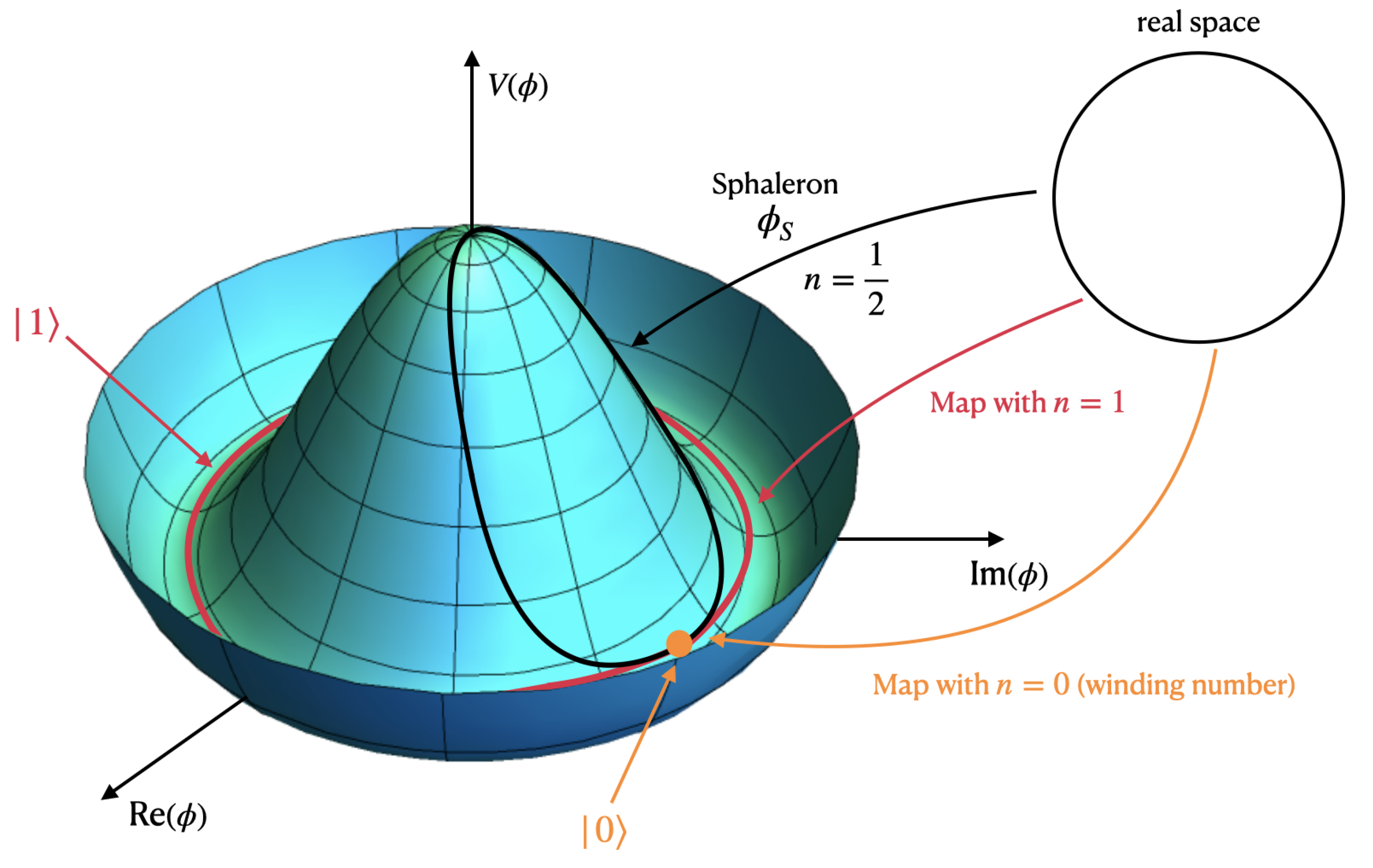
Because of the periodicity on , should be periodic but we could also consider that , where . These transformations will define the so-called large gauge transformations. One particularly interesting transformation is defined with . In that case, our vacuum will be transformed into and , which we will define as . Each of these solutions have zero energy and therefore constitute a different vacuum.
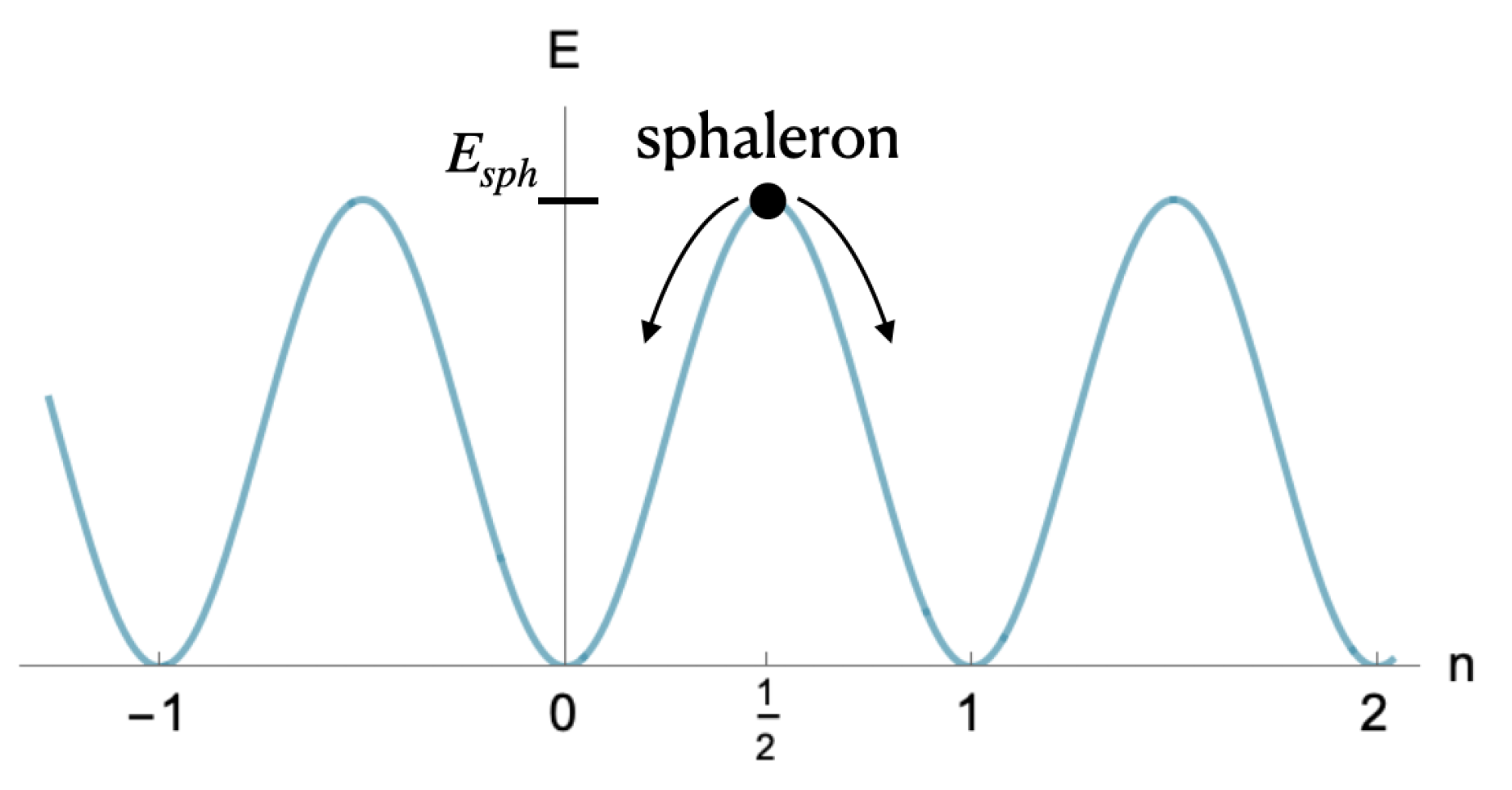
As can be seen from Figure 3, these solutions cannot be deformed one into the other if we remain at zero energy; they are not continuous path deforming of into . However, they can be connected by a solution which is not the vacuum and therefore have non-zero energy and pass by the maximum of the potential [10]. This corresponds to the sphaleron configuration with energy . This solution permits us to go from to or more generically from to (and inversely).
Considering , we have:
which is our kink solution found for the ungauged case ) under the large gauge transformation with (see Figure 4 to build a simple intuition of the value ).
This solution has an energy,
with the mass of the “Higgs” field (scalar field ). Notice that, at the quantum level, we can have quantum tunnelling between two vacua, known as instanton, but which are irrelevant for our topic. At high temperatures, the system can have enough energy to trigger this transition which is known as sphaleron.
4.3. Violation of the Baryon Number
As we have seen previously, the vacuum can have a rich structure and we could have transitions from one into the other if enough energy is provided. This transition represents a violation of the baryon (lepton) number. In order to demonstrate it, let us continue with our toy model [11] by introducing fermions,
where , and are matrices satisfying , with . We can take
and define
We have two global symmetries corresponding to and , leading to conservation (via the Noether theorem) to vector and axial currents and , to which we can associate the charges and .
It can be shown using different methods that is not conserved at the quantum level. We will see later Fujikawa’s approach [12,13], which is the most powerful method, but in this section, the problem being two dimensional, we can prove the non-conservation of in a simpler way.
We label the components of as which gives:
Considering for the moment, the problem with , we have:
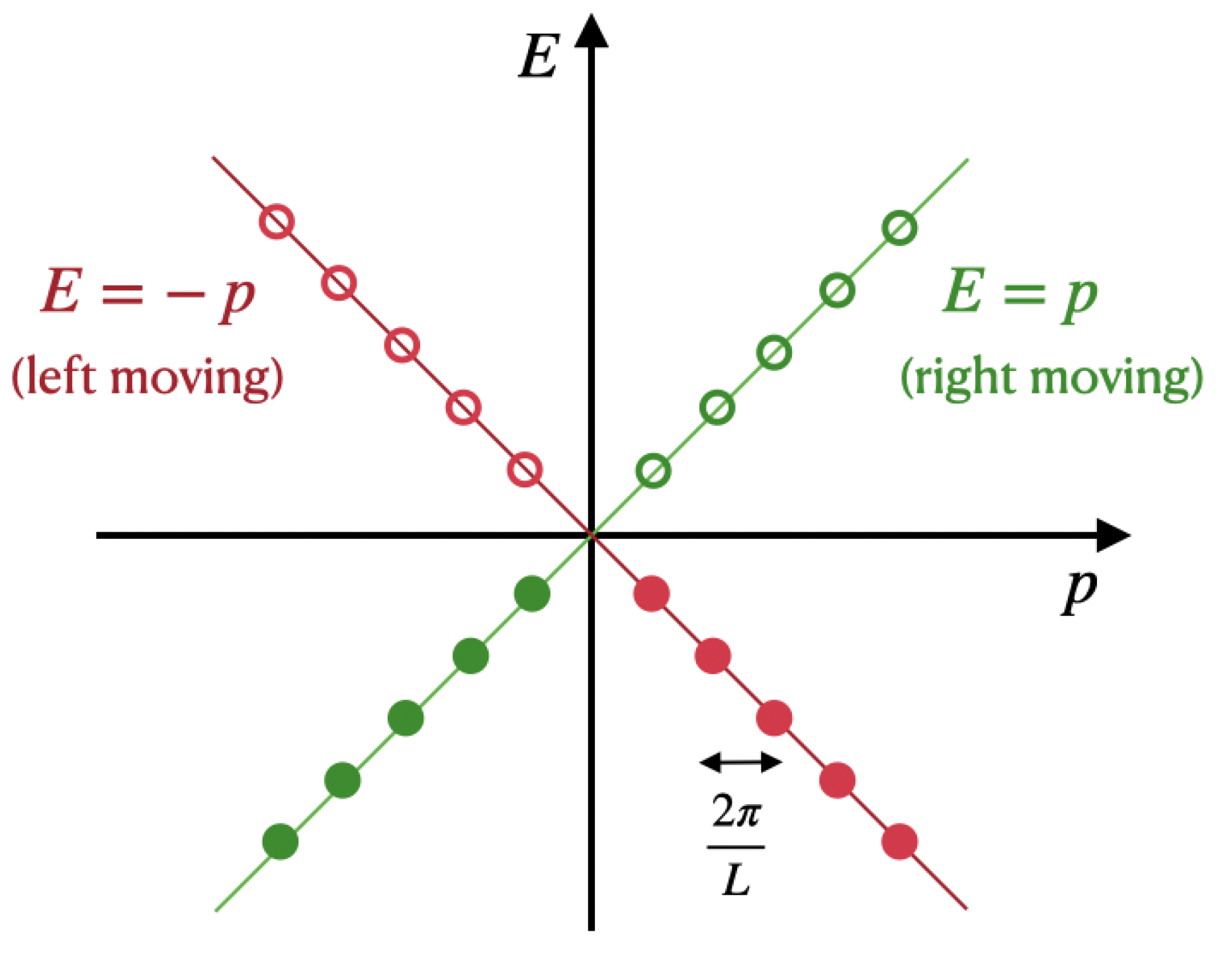
which implies and , so is left moving (towards decreasing x) and is right moving. Notice that so is a left-handed spinor while is right-handed. We define the normalised wave functions and but because the generic form of a wave is we deduce that for and for . Notice also that with because of the periodicity condition. We can write:
where annihilates a particle with positive energy and momentum and does the same but with a particle . Similarly, creates an antiparticle with positive energy and for left- and right-handed antiparticles (the destruction of particles with negative energy is written into antiparticles of positive energy). We also have the standard relation and this is similar for the other operators. The vacuum corresponds to all negative energies filled as shown in Figure 5.
As we have mentioned, because of the two global symmetries, we have two conserved charges,
where we have used the relation of orthogonality , which implies
Notice that we have eliminated the divergent term, , which comes from the relation . In conclusion, we have:
while
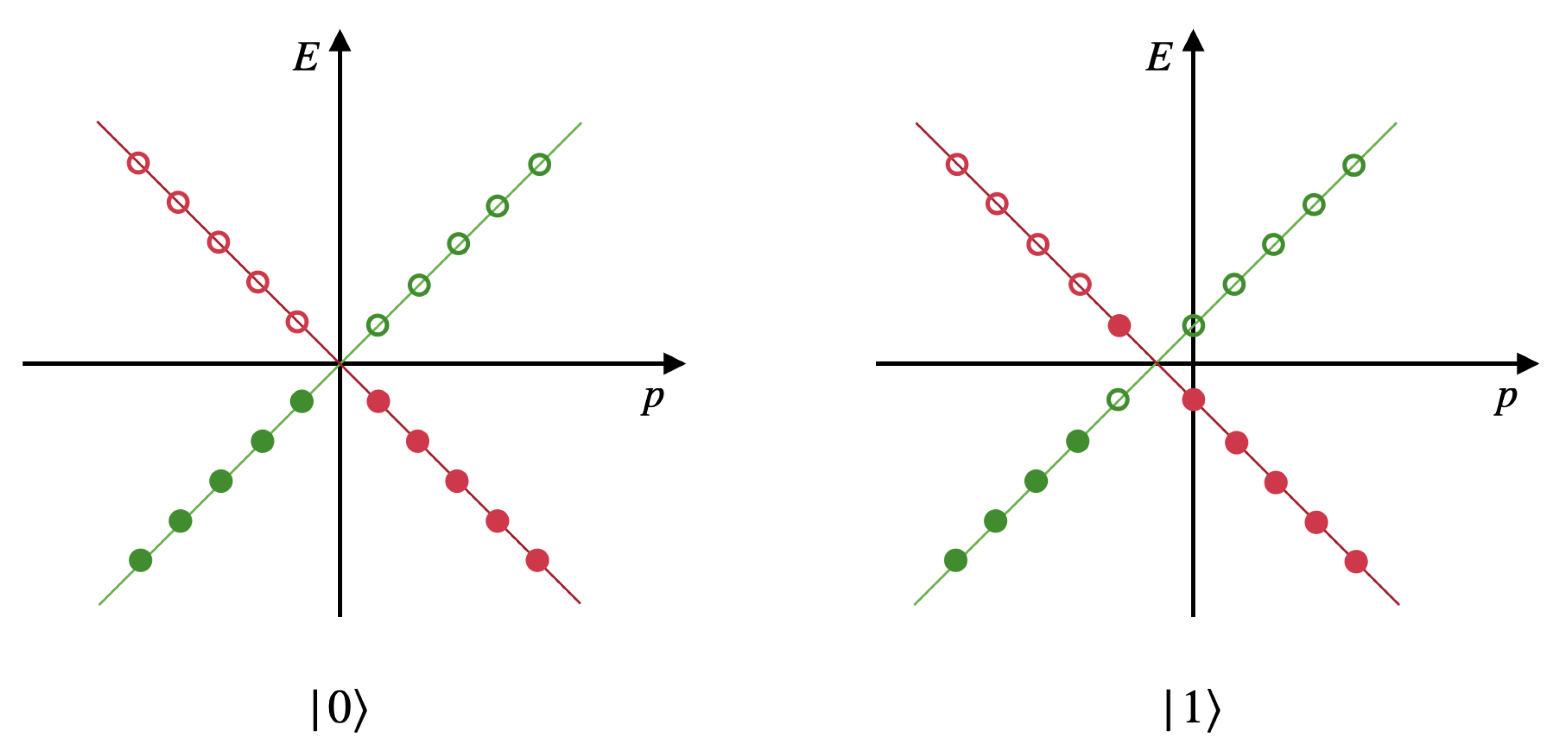
These two charges should be conserved, but in the presence of the potential , changes, so is not conserved. To prove it, let us consider the presence of a gauge field as an external and not a dynamical field; is fixed. We know that it corresponds to the substitution . Therefore, when increases, p decreases. Let us consider the transition from (from our vacuum ) to the vacuum corresponding to , which means a shift that corresponds to one quanta of energy. For right-handed particles the energy changes as , while for left-handed particles we have (because ).
We see from Figure 6 that we have the creation of a left-handed particle and the destruction of a right handed particle. So, we have ; therefore it is conserved while is not conserved.
Indeed, as we will see in the next subsection,
which implies
Using a toy model, we have seen that the number of left- and right-handed particles are not conserved. The axial charge is not conserved in the presence of the gauge field corresponding to another vacuum. In conclusion, the action of changing the vacuum because of the sphaleron changes the baryon number.
4.4. Fujikawa’s Method
A conserved classical charge which is not conserved in the quantum realm is known as an anomaly. Fujikawa has shown [12] that, using the path integral approach, the measure of the functional integral is not invariant. Let us as a first approximation eliminate the Higgs field and build our partition function,
Let us consider the infinitesimal change of variable
The action changes as
where we used that . If the measure in the definition of the partition function was invariant, we would get
Since we performed a change of variables, the partition function should remain the same and therefore we obtain the Ward identity , which is the analogue of the classical Noether conservation equation. However, the measure is not gauge-invariant which implies an anomalous Ward identity. In order to see how the measure transforms, we need to better define it. For that, we define a complete set of eigenfunctions of the operator
with the inner product
We can expand in these bases, and , which implies , where are Graßmann variables. Additionally, because , we obtain for the transformation (40)
and
which implies that the Jacobian of the transformation is
using the identity we obtain
where Tr’ represents the trace over spinor indices. Such an infinite sum is divergent. To regularize it, we redefine the summation as . The regulator could be any function such that and rapidly approaches 0 for large .
Therefore, because which implies
Because trace is invariant, we can express it in any basis and therefore in the momentum basis. We get:
However, we know that , therefore
Using that , we have:
where we defined on the second line. We can now perform a series expansion for . All terms without any gamma matrix, , will disappear after taking the trace over Dirac indices. Indeed, these elements will be multiplied by and . Similarly, the terms will vanish because in four dimensions. Therefore, the first non-zero term will be
higher order terns will be suppressed in the limit
To calculate the trace, we notice that, if two indices are equal, we are back to which is zero. Therefore all indices are different and, because in that case , we conclude that . Taking , we obtain where we used that
Let us remember that , therefore for the integral we perform a wick rotation
In order to obtain the Lorentzian version, we transform (because
In conclusion, we found that, under the transformation , we have
Finally, the partition function gives at first order:
which gives the Adler–Bell–Jackiw anomaly [14,15]:
Notice that, in two dimensions, the calculation would be similar:
Therefore, the first non-zero contribution is:
Taking the trace and using that in two dimensions, , we obtain or
giving
The chiral anomaly is at the origin of the non-conservation of baryon and lepton numbers.
5. Baryon and Lepton Number Conservation
In the Standard Model of particle physics, we have global symmetries for quark and lepton fields:
The factor 3 for quarks is included to have a unit baryon number for particles such as protons. These symmetries imply, classically, two conserved currents,
where implicitly we considered a summation over all quarks and all leptons. The associated charge numbers are and . These currents are vectorial, therefore we should not expect a violation of these numbers, contrary to axial currents. However, in the Standard Model, only left-handed particles couple to weak gauge bosons. This violates parity and therefore these numbers are not conserved, B and L are anomalous. Notice also that an additional anomaly comes from the coupling to the weak hypercharged boson but that will be almost irrelevant. Following the same previous strategy but defining the gauge covariant derivative as , we will have to replace e by and sum over the six types of quarks or six types of leptons, finally giving a factor ,
We have an additional trace for internal group indices because now we have a non-abelian gauge theory:
where are the gauge fields and the generators of . Notice that , so is conserved while B and L are not conserved, which is often summarised as is not conserved while is conserved.
Similarly to the previous case, where we introduced a current , we have:
Taking the trace, we obtain for the last term because is completely antisymmetric while the trace is cyclic. Finally, we also have: , which gives:
If we write this equation in components, we have , where are the generators of the Lie algebra . We use the normalisation , which implies symmetric part (obtained from and multiplying by ,
or equivalently 4
Integrating this relation over space and time, we obtain:
with . Defining the Chern–Simons number as:
we obtain . However, because 5 we have in such processes a group of three leptons and three baryons (or nine quarks) involved, such as (13). Notice that, because the group involved is , only left-handed particles and right-handed antiparticles are involved in such processes.
6. Limits of the Standard Model
In summary, to possibly solve the BAU we need to comply with the three Sakharov conditions.
- The non-equilibrium condition seems to be obviously reached because the universe is expanding.
- The baryon number violation exists in the SM because of the rich structure of the vacuum and transitions between them. We have constructed the sphaleron in the simple abelian theory; the sphaleron [16,17] can be derived using the minimax procedure [18]. Notice that we can also have a change of vacuum via quantum tunnelling, which is known as instanton, but that would be highly suppressed [19]. The probability of tunnelling can be calculated with the help of the euclidean partition function which is dominated by the saddle point configuration, giving a probability of order , where we used .
- Finally, to meet the three Sakharov conditions, we need C and violation. C and are violated in the standard model because of terms such as:where , are the left handed quarks, is the W boson, the weak gauge coupling and, finally, the Cabibbo–Kobayashi–Maskawa mixing matrix. The CP symmetry is violated if the phase angle in the CKM matrix is , which has been verified experimentally [7]. Therefore, we have violation processes in the SM. Notice that from neutrino mixing, the PMNS matrix (Pontecorvo–Maki–Nakagawa–Sakata) could also be complex and hence produce an additional CP violation.
Unfortunately, even if all conditions are met, the asymmetry produced would not be sufficient. Indeed, the sphaleron process plays against us at high temperatures. From lattice simulations [20], the sphaleron rate is found to be at high temperatures,
while this rate is exponentially suppressed at low temperatures,
These rates should be contrasted with the expansion rate, defined as the Hubble rate , during the radiation era. From the formulae defined in the Appendix A, we obtain at high temperature,
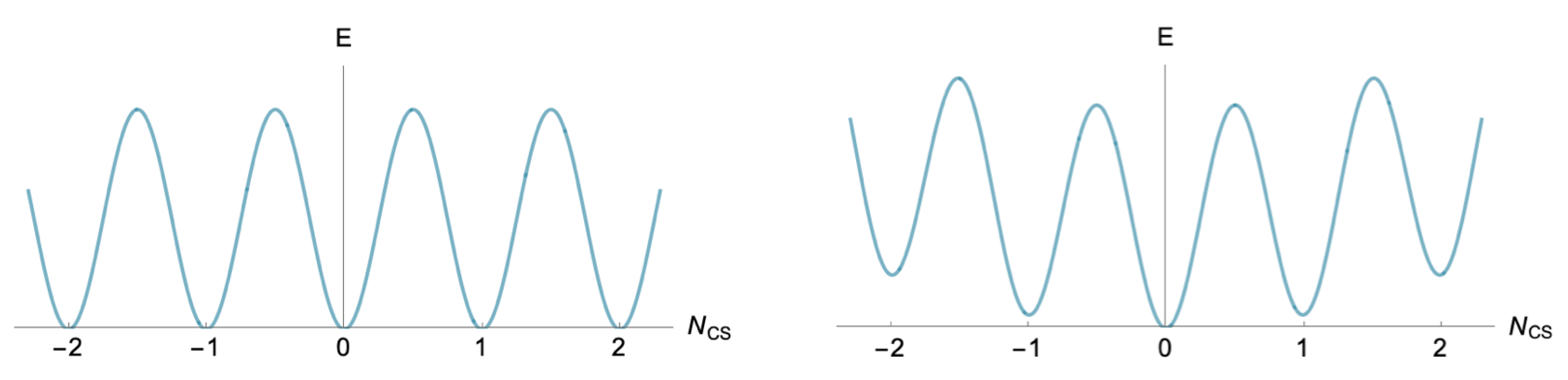
with , which gives the baryon freeze-out temperature 6 (by comparing both rates) as . Consequently, for , the sphaleron process is suppressed. Instead, at higher temperatures, the sphaleron rate can be large and therefore we have processes creating baryons and leptons; for example, the process (13), for which and . Unfortunately, this picture is a bit simplistic, because producing more and more fermions costs energy. In their presence, the vacuum previously shown is modified [21,22] as shown in Figure 7. So, the system tends to ; this is the washout process. Therefore, any asymmetry will be suppressed.
Another problem is related to CP violation in the Standard Model. It is too small [23] to generate the observed baryon asymmetry. Finally, we need a much more violent process than the expansion of the universe to go out of equilibrium. For that, and considering the freeze-out temperature, we see that electroweak phase transition could be such an out-of-equilibrium process. Unfortunately, this phase transition is not first order but a crossover in the SM [24,25].
In summary, a viable electroweak baryogenesis model needs physics beyond the Standard Model. We will not here detail the various possible extensions. We will assume that we added into our Lagrangian violating terms and made the phase transition first order 7.
7. Electroweak Baryogenesis
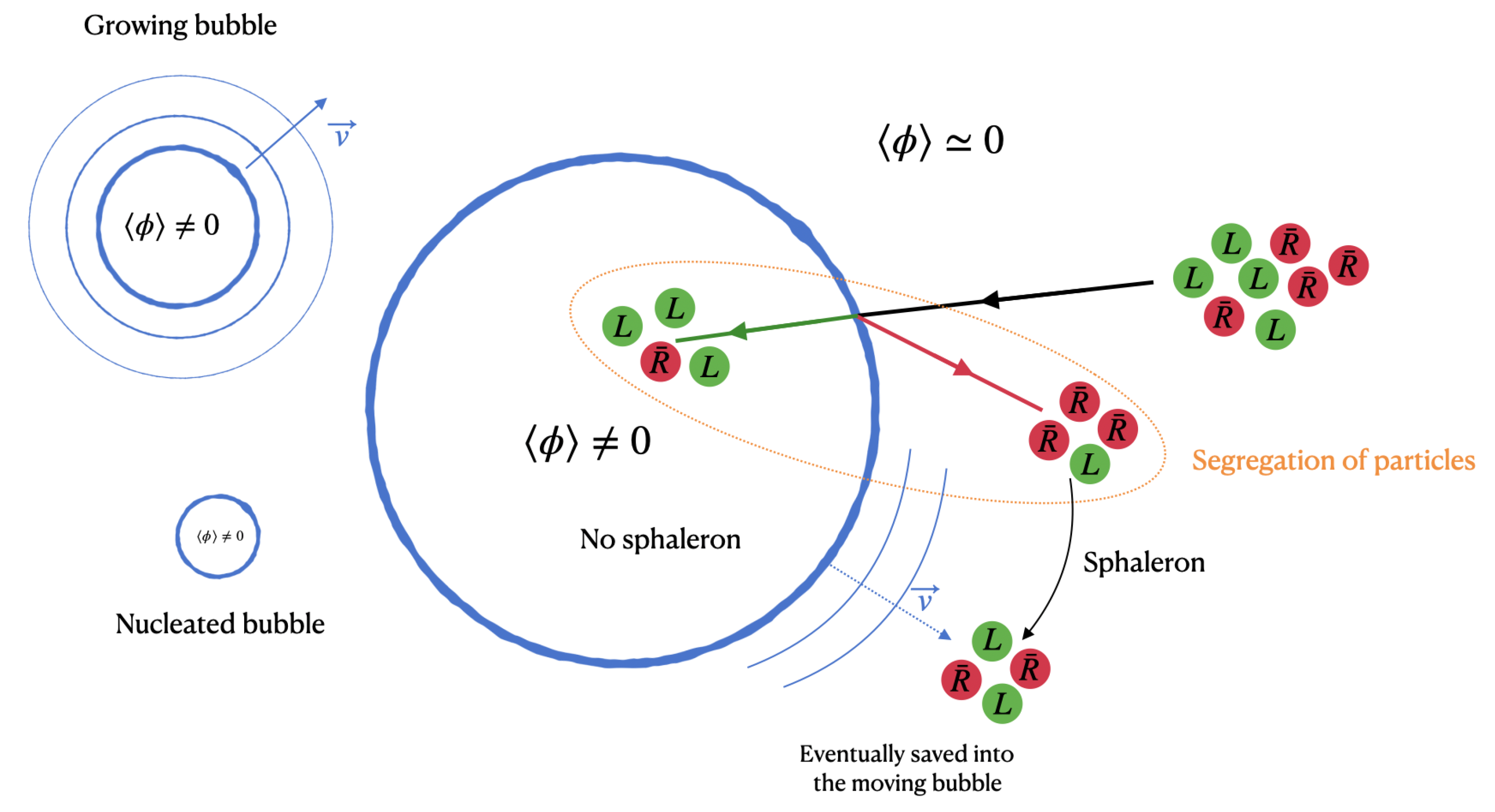
The Higgs field dynamics is guided by a potential which receives quantum and thermal contributions. Therefore, the potential changes with time which in return changes the VEV of the Higgs field. If initially the potential has a minimum at , it will take a different value of around . Of course this process cannot happen in the whole universe at the same time, therefore bubbles will nucleate, grow if they are large enough and collapse if they are too small, see e.g., [28] for more details of this process. Let us look at one bubble in particular. In the symmetric phase (as we have said, it is an abuse of language), particles are almost massless while they are massive in the broken phase (inside the bubble) because the Higgs field takes a large VEV. Let us consider a top quark which will be the most massive in the broken phase. If in the symmetric phase a top quark has an energy , it will bounce over the bubble wall; because top quarks are massive inside the bubble, it appears as a barrier. On the contrary, if the top quark has large energy, it will penetrate the bubble. In general, we will have some transmission and refection of these particles. These coefficients will depend on the extension of the SM that we built and in particular the C and CP violation introduced in the Lagrangian. Let us suppose that we tuned the parameters of our beyond Standard Model such that reflection and transmission coefficients are different between particles and antiparticles and also their helicity. For example, we could have an excess of right-handed antiparticles in the exterior because of the CP violating bubble interactions. For the moment, we have not built any asymmetry but only segregated particles, as we can see from Figure 8.
In general, we could have a sphaleron process producing an excess of baryons (growing ) or antisphaleron (decreasing ). However, because we have an excess of antibaryons, the sphaleron process will be more probable than the antisphaleron. Therefore, we are ending with antibaryons converted into baryons 8. This net baryon asymmetry could be easily washed out by an inverse process. This is why the speed of the growing bubble will be very relevant and therefore only processes occurring near the bubble are important. Sphalerons occurring far from the bubble wall will be washed out before the wall arrives in that region. The freshly produced particles will interact with the moving bubble and some will enter inside where the sphaleron process is suppressed and therefore the asymmetry conserved. Of course this mechanism, known as electroweak baryogenesis (EWBG), relies on various phenomena that we have not described. This short review tried to introduce the basic knowledge for a viable EWBG. In order to calculate an exact amount of baryon asymmetry, a specific model should be assumed, such as MSSM (Minimal Supersymmetric Standard Model) or 2HDM (Two Higgs Doublet Model). For a given model, the energy of the sphaleron can be calculated along with thermal corrections to the Higgs potential, which gives rise to the rate and the temperature of bubble nucleation. Of course, the model will rely strongly on the transmission and reflection coefficients which are guided by the quantum transport equations, see e.g., [29] for a nice review. Finally, the properties of the moving wall are very important, such as the width and speed in a complex plasma interacting with it [28].
8. Conclusions
The universe is mostly filled with matter while antimatter is missing. The observed antimatter is secondary origin. This is the problem of baryon asymmetry, which has led to a rich and complex field of research. One of the most popular models has been the electroweak baryogenesis because all the ingredients for its realisation exist in the Standard Model. Unfortunately, the asymmetry produced is not sufficient and therefore it calls for an extension of the Standard Model of particle physics. This review introduced a general overview of the mechanism focusing principally on aspects that are less detailed in other documents. Of course, many other mechanisms exist in the market and a recent state-of-the-art can be found in [30].
Funding
This work was supported by the grant Fondecyt n°1220965.
Institutional Review Board Statement
Not applicable.
Informed Consent Statement
Not applicable.
Acknowledgments
I would like to thank M. Sami for inviting me to write this review.
Conflicts of Interest
The author declares no conflict of interest.
Appendix A. Number of Photons
Particles can be described as a perfect Fermi or Bose gas with the help of the distribution function
where the ± sign correspond to Fermi-Dirac or Bose-Einstein statistics. The energy of the system is E, the chemical potential and T the temperature of the gas.
From the distribution function, we can define the different macroscopic variables such as the number of particles
where g is the degeneracy of the element, or internal degrees of freedom. The average energy is
the (scalar) pressure
and the entropy
for bosons and fermions respectively. Assuming that the different particles form a gas in equilibrium in a homogeneous and isotropic universe, we can simplify the expression because . Therefore we obtain
where we have used and defined , and . Similarly, we have
and
When and , we have
which implies
where we have used for all species [31] and the degeneracy factors are summarized in the following tables
| Fermions | Quarks Antiquarks | Leptons Antileptons | Neutrinos Antineutrinos |
| g |
| Bosons | Photon | Z | Gluons | Higgs boson | ||
| g | 2 | 3 | 3 | 3 | 1 |
Appendix B. Entropy
Let us consider that our system is described by the grand canonical ensemble, with J the grand potential and Z the partition function, which defines
where . If we consider that we have a fluid with short range interactions, each subsystem of the total system can be described by a grand potential, while the total grand potential is the sum of these potentials. Therefore J grows like the volume, i.e., it is an extensive variable. In that case, if ), we have but because which gives and therefore
which implies
where we reestablished the coefficient c in the last expression and neglected the chemical potential. We have
where it is implicitly assumed a summation over all species. The main contribution comes from relativistic particles such as photons at temperature and neutrinos with temperature , which gives and therefore
| 1 | CMB was discovered in 1965, 2 years before Sakharov’s conditions. |
| 2 | We defined . |
| 3 | At high temperatures, the chemical potential is very small, while it increases when particles become non-relativistic. Fortunately, the contribution to entropy of non-relativistic particles is exponentially suppressed. |
| 4 | The formulas are given with details because some confusion exists in the literature. |
| 5 | See e.g., [10] on why is an integer. |
| 6 | Temperature at which a process goes back to equilibrium, with only a dilution produced by the expansion of the universe. |
| 7 | A Higgs field in the fundamental representation coupled to has no gauge-invariant order parameter [26,27]. Therefore, it makes it difficult to speak of broken and symmetric phases. The Higgs field could have a non-zero VEV in the early universe and change to a larger value at later time instead of a phase transition as often abusively mentioned in the literature. |
| 8 | Of course, in each process, nine quarks/antiquarks and three leptons/antileptons are involved such that is conserved. Therefore, we have a production of baryons and leptons, as in the example (13). |
References
- Caprini, C.; Hindmarsh, M.; Huber, S.; Konstandin, T.; Kozaczuk, J.; Nardini, G.; No, J.M.; Petiteau, A.; Schwaller, P.; Servant, G.; et al. Science with the space-based interferometer eLISA. II: Gravitational waves from cosmological phase transitions. JCAP 2016, 4, 001. [Google Scholar] [CrossRef] [Green Version]
- Rubakov, V.A.; Shaposhnikov, M.E. Electroweak baryon number nonconservation in the early universe and in high-energy collisions. Usp. Fiz. Nauk 1996, 166, 493–537. [Google Scholar] [CrossRef] [Green Version]
- Trodden, M. Electroweak baryogenesis. Rev. Mod. Phys. 1999, 71, 1463–1500. [Google Scholar] [CrossRef] [Green Version]
- Riotto, A. Theories of baryogenesis. arXiv 1998, arXiv:hep-ph/9807454. [Google Scholar]
- Cline, J.M. Baryogenesis. arXiv 2006, arXiv:hep-ph/0609145. [Google Scholar]
- Morrissey, D.E.; Ramsey-Musolf, M.J. Electroweak baryogenesis. New J. Phys. 2012, 14, 125003. [Google Scholar] [CrossRef]
- [Particle Data Group]; Workman, R.L.; Burkert, V.D.; Crede, V.; Klempt, E.; Thoma, U.; Tiator, L.; Agashe, K.; Aielli, G.; Allanach, B.C.; et al. Review of Particle Physics. PTEP 2022, 2022, 083C01. [Google Scholar]
- Pitrou, C.; Coc, A.; Uzan, J.P.; Vangioni, E. Precision big bang nucleosynthesis with improved Helium-4 predictions. Phys. Rept. 2018, 754, 1–66. [Google Scholar] [CrossRef] [Green Version]
- Aghanim, N.; Akrami, Y.; Ashdown, M.; Aumont, J.; Baccigalupi, C.; Ballardini, M.; Banday, A.J.; Barreiro, R.B.; Bartolo, N.; Basak, S.; et al. Planck 2018 results. VI. Cosmological parameters. Astron. Astrophys. 2020, 641, A6, Erratum in Astron. Astrophys. 2021, 652, C4. [Google Scholar]
- Manton, N.S.; Sutcliffe, P. Topological Solitons; Cambridge University Press: Cambridge, UK, 2004. [Google Scholar]
- Nielsen, H.B.; Ninomiya, M. Adler-bell-jackiw anomaly and weyl fermions in crystal. Phys. Lett. B 1983, 130, 389–396. [Google Scholar] [CrossRef]
- Fujikawa, K. Path Integral Measure for Gauge Invariant Fermion Theories. Phys. Rev. Lett. 1979, 42, 1195–1198. [Google Scholar] [CrossRef]
- Fujikawa, K.; Suzuki, H. Path Integrals and Quantum Anomalies; Oxford University Press: Oxford, UK, 2004. [Google Scholar]
- Adler, S.L. Axial vector vertex in spinor electrodynamics. Phys. Rev. 1969, 177, 2426–2438. [Google Scholar] [CrossRef] [Green Version]
- Bell, J.S.; Jackiw, R. A PCAC puzzle: π0→γγ in the σ model. Nuovo Cim. A 1969, 60, 47–61. [Google Scholar] [CrossRef] [Green Version]
- Klinkhamer, F.R.; Manton, N.S. A Saddle Point Solution in the Weinberg-Salam Theory. Phys. Rev. D 1984, 30, 2212. [Google Scholar] [CrossRef]
- Manton, N.S. Topology in the Weinberg-Salam Theory. Phys. Rev. D 1983, 28, 2019. [Google Scholar] [CrossRef]
- Klinkhamer, F.R.; Rupp, C. Sphalerons, spectral flow, and anomalies. J. Math. Phys. 2003, 44, 3619–3639. [Google Scholar] [CrossRef]
- Hooft, G.T. Computation of the Quantum Effects Due to a Four-Dimensional Pseudoparticle. Phys. Rev. D 1976, 14, 3432–3450, Erratum in Phys. Rev. D 1978, 18, 2199. [Google Scholar] [CrossRef]
- D’Onofrio, M.; Rummukainen, K.; Tranberg, A. Sphaleron Rate in the Minimal Standard Model. Phys. Rev. Lett. 2014, 113, 141602. [Google Scholar] [CrossRef] [Green Version]
- Kuzmin, V.A.; Rubakov, V.A.; Shaposhnikov, M.E. On the Anomalous Electroweak Baryon Number Nonconservation in the Early Universe. Phys. Lett. B 1985, 155, 36. [Google Scholar] [CrossRef]
- Cohen, A.G.; Kaplan, D.B.; Nelson, A.E. Progress in electroweak baryogenesis. Ann. Rev. Nucl. Part. Sci. 1993, 43, 27–70. [Google Scholar] [CrossRef]
- Gavela, M.B.; Hernandez, P.; Orloff, J.; Pene, O. Standard model CP violation and baryon asymmetry. Mod. Phys. Lett. A 1994, 9, 795–810. [Google Scholar] [CrossRef] [Green Version]
- Kajantie, K.; Laine, M.; Rummukainen, K.; Shaposhnikov, M.E. Is there a hot electroweak phase transition at mH≳mW? Phys. Rev. Lett. 1996, 77, 2887–2890. [Google Scholar] [CrossRef] [PubMed] [Green Version]
- Rummukainen, K.; Tsypin, M.; Kajantie, K.; Laine, M.; Shaposhnikov, M.E. The Universality class of the electroweak theory. Nucl. Phys. B 1998, 532, 283–314. [Google Scholar] [CrossRef] [Green Version]
- Fradkin, E.H.; Shenker, S.H. Phase Diagrams of Lattice Gauge Theories with Higgs Fields. Phys. Rev. D 1979, 19, 3682–3697. [Google Scholar] [CrossRef]
- Fradkin, E.H. Field Theories of Condensed Matter Physics. Front. Phys. 2013, 82, 1–852. [Google Scholar]
- Hindmarsh, M.B.; Lüben, M.; Lumma, J.; Pauly, M. Phase transitions in the early universe. SciPost Phys. Lect. Notes 2021, 24, 1. [Google Scholar] [CrossRef]
- Konstandin, T. Quantum Transport and Electroweak Baryogenesis. Phys. Usp. 2013, 56, 747–771. [Google Scholar] [CrossRef] [Green Version]
- Elor, G.; Harz, J.; Ipek, S.; Shakya, B.; Blinov, N.; Co, R.T.; Cui, Y.; Dasgupta, A.; Davoudiasl, H.; Elahi, F.; et al. New Ideas in Baryogenesis: A Snowmass White Paper. arXiv 2022, arXiv:2203.05010. [Google Scholar]
- Fixsen, D.J. The Temperature of the Cosmic Microwave Background. Astrophys. J. 2009, 707, 916–920. [Google Scholar] [CrossRef]
Figure 1.
Because weak interactions do not conserve strangeness, we can have these types of box diagrams representing the transformation of a neutral kaon into its antiparticle.
Figure 1.
Because weak interactions do not conserve strangeness, we can have these types of box diagrams representing the transformation of a neutral kaon into its antiparticle.

Figure 2.
Complex kink solution, which corresponds to the mapping from to the scalar field space.

Figure 3.
Representation in the scalar field space of the two vacua solutions , and also the solution connecting them, known as the sphaleron, which has an unstable direction. The sphaleron and the vacua appear as a mapping between the real space and a circle in the field space. The homotopy class associated will be non trivial , where this number is often known as the winding number.

Figure 4.
Visualization of the sphaleron configuration between two degenerate vacua. It corresponds to an unstable structure of the half integer Chern–Simons number. If the temperature is large enough, the sphaleron can be created and its instability can make it decay into one of the two vacua with or in our particular case.

Figure 5.
Spectrum for the left-handed and right-handed fermions with all negative energies filled corresponding to the Dirac sea and therefore to our vacuum.
Figure 5.
Spectrum for the left-handed and right-handed fermions with all negative energies filled corresponding to the Dirac sea and therefore to our vacuum.

Figure 6.
Effect on the energy spectrum because of the presence of a non-zero gauge potential. We see that a left-handed particle (red) is created while a right-handed particle (green) is destroyed.
Figure 6.
Effect on the energy spectrum because of the presence of a non-zero gauge potential. We see that a left-handed particle (red) is created while a right-handed particle (green) is destroyed.

Figure 7.
In the left-hand side of the figure, the vacuum structure studied previously is shown, while in the right-hand figure, we have the vacuum structure in the presence of fermions,. We see that a particular vacuum will be preferred, which corresponds to . This is the washout process.
Figure 7.
In the left-hand side of the figure, the vacuum structure studied previously is shown, while in the right-hand figure, we have the vacuum structure in the presence of fermions,. We see that a particular vacuum will be preferred, which corresponds to . This is the washout process.

Figure 8.
Sketch of electroweak baryogenesis based on nucleated bubbles and their growth. In this sketch, an equal amount of left-handed particles and right-handed antiparticles are considered (the right-handed particles and left-handed antiparticles are not participating in a sphaleron process). After particles are segregated—this is the chiral asymmetry—they are converted into a baryon asymmetry before being swallowed by the fast moving bubble.

Publisher’s Note: MDPI stays neutral with regard to jurisdictional claims in published maps and institutional affiliations. |
© 2022 by the author. Licensee MDPI, Basel, Switzerland. This article is an open access article distributed under the terms and conditions of the Creative Commons Attribution (CC BY) license (https://creativecommons.org/licenses/by/4.0/).
Share and Cite
MDPI and ACS Style
Gannouji, R. Introduction to Electroweak Baryogenesis. Galaxies 2022, 10, 116. https://doi.org/10.3390/galaxies10060116
AMA Style
Gannouji R. Introduction to Electroweak Baryogenesis. Galaxies. 2022; 10(6):116. https://doi.org/10.3390/galaxies10060116
Chicago/Turabian StyleGannouji, Radouane. 2022. "Introduction to Electroweak Baryogenesis" Galaxies 10, no. 6: 116. https://doi.org/10.3390/galaxies10060116
Note that from the first issue of 2016, this journal uses article numbers instead of page numbers. See further details here.