

Data Analysis of Impaired Renal and Cardiac Function Using a Combination of Standard Classifiers
 , , , and
Abstract
:1. Introduction
2. Methods
2.1. Patient Selection
2.2. Laboratory Analysis and Data Collection
2.3. Equation Estimating GFR
2.4. Statistical Analysis
3. Computer-Based Classification Using Standard Classifiers
4. Stable and Unstable Predictors
5. Representativeness and Generalization
5.1. Representativeness of the Samples
5.2. Forecasting Ensembles
- (a)
- Creation of a set of models: Construction of different individual members of the ensemble.
- Combining different learning methods (heterogeneous ensembles) or combining the architecture and complexity of one learning method (homogeneous ensembles);
- Manipulation of the available training data set.
- (b)
- Reduction: Removing weak and redundant models:
- (c)
- Integration: combining selected models:
5.3. Bootstrap Aggregation
6. Applied Classifiers
6.1. Multilayer Perceptron
6.2. k-Nearest Neighbors Classifier
6.3. Naive Bayes Classifier
6.4. Decision Trees
6.5. Logistic Regression
7. Performance and Metrics of Classifiers
8. Feature Subset Selection
9. Results
9.1. Study Population
9.2. Training Data

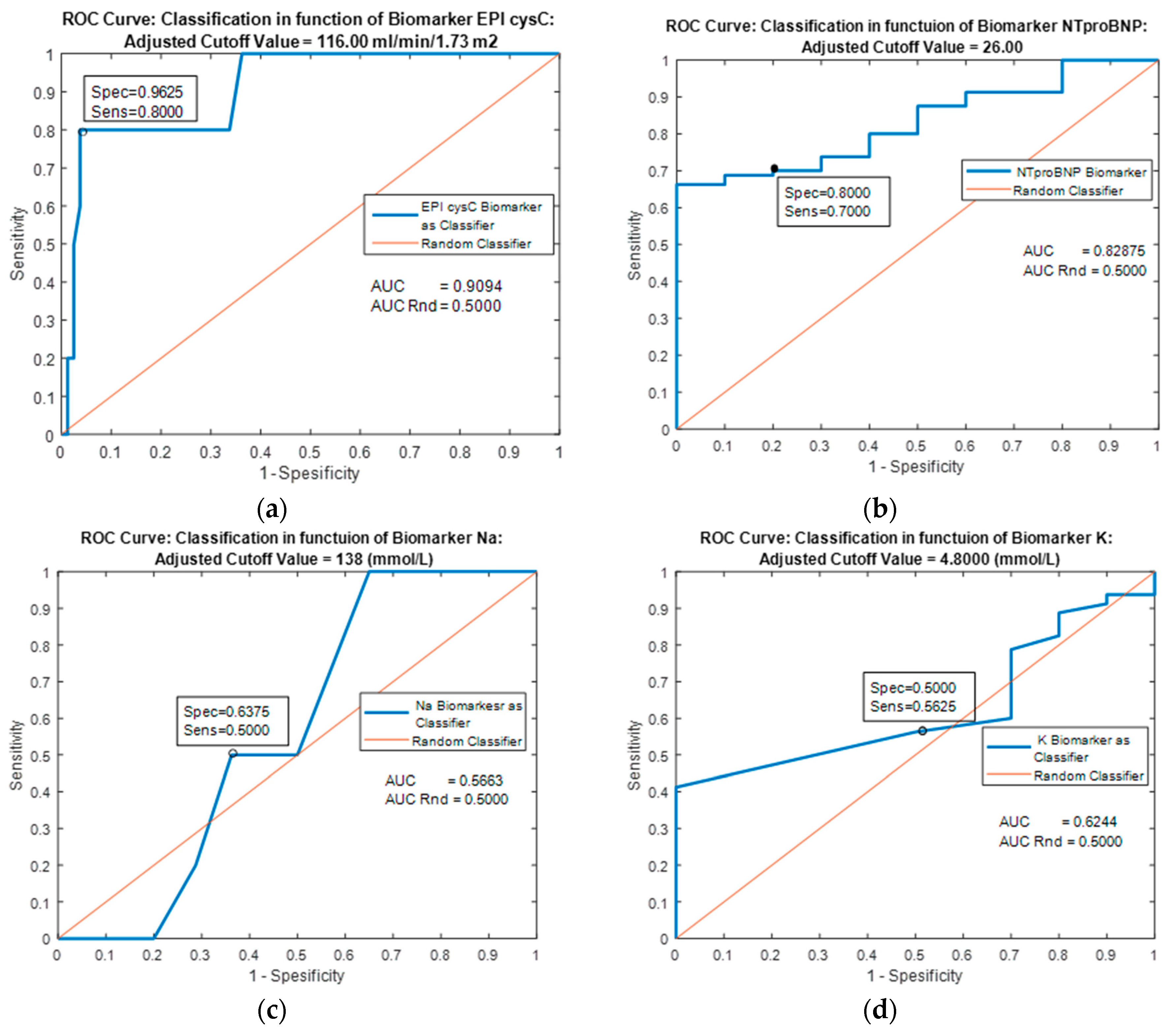
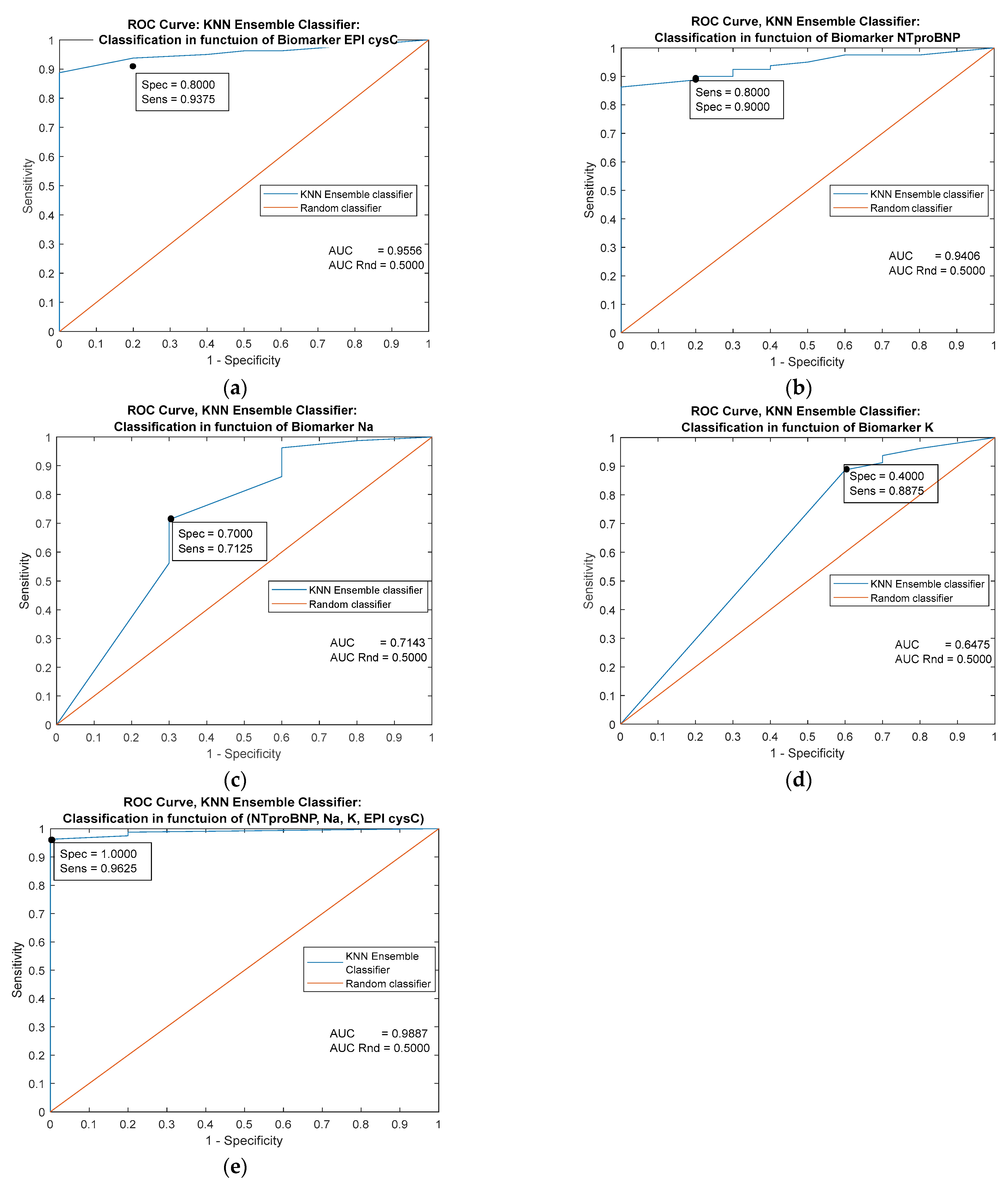
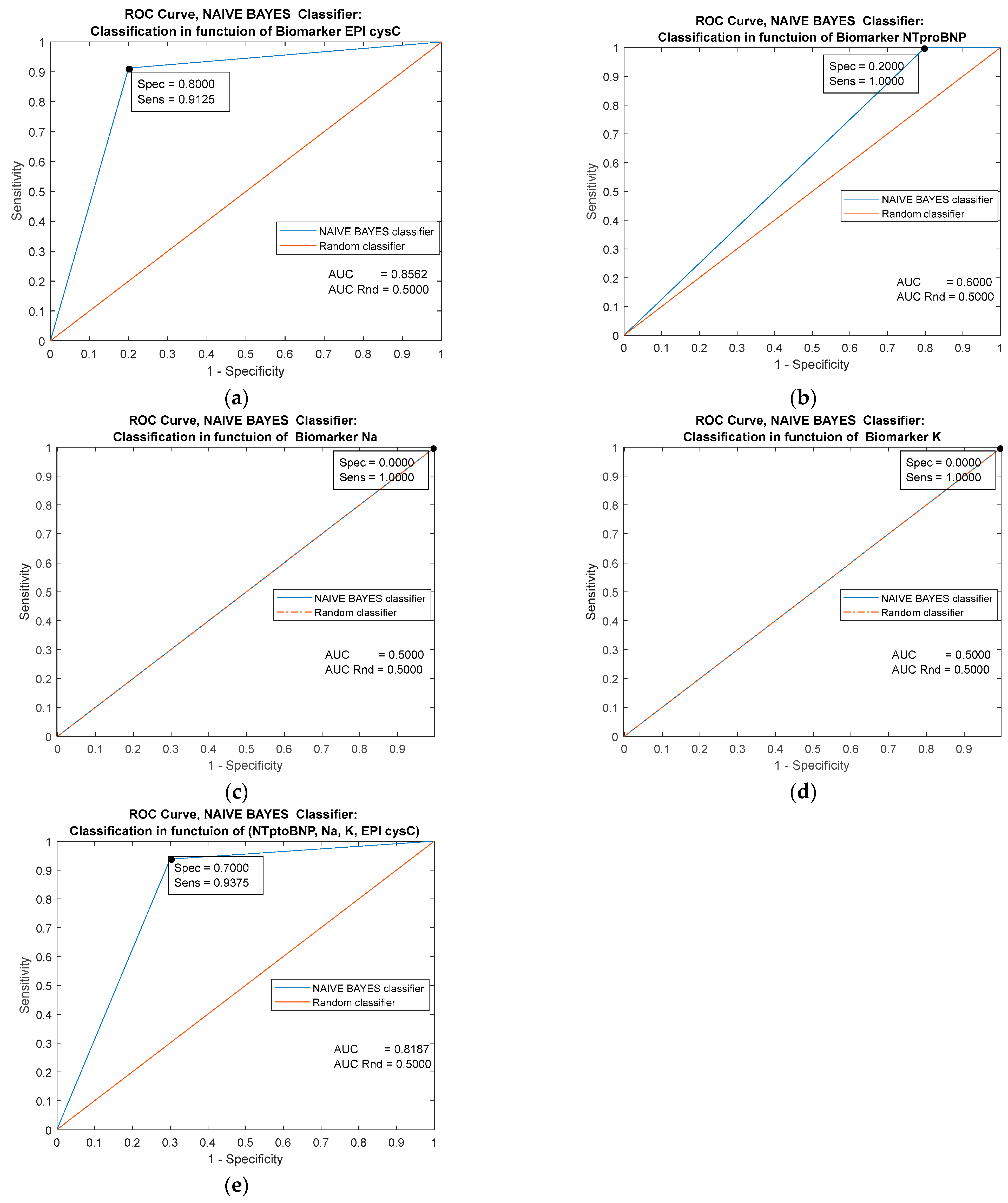
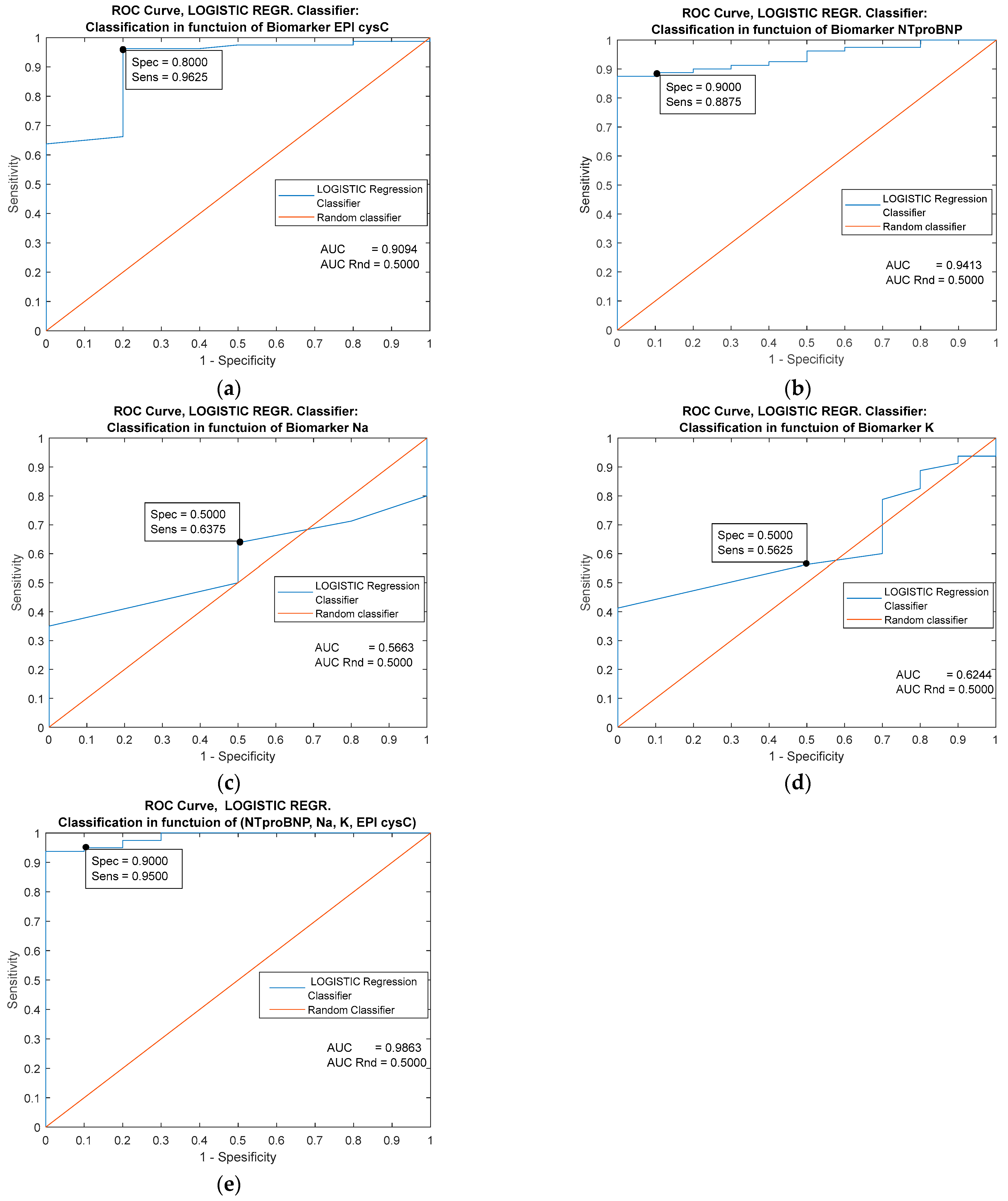
| Predictor | Single Biomarker: EPI cysC (mL/min/1.73 m2) | |||||
|---|---|---|---|---|---|---|
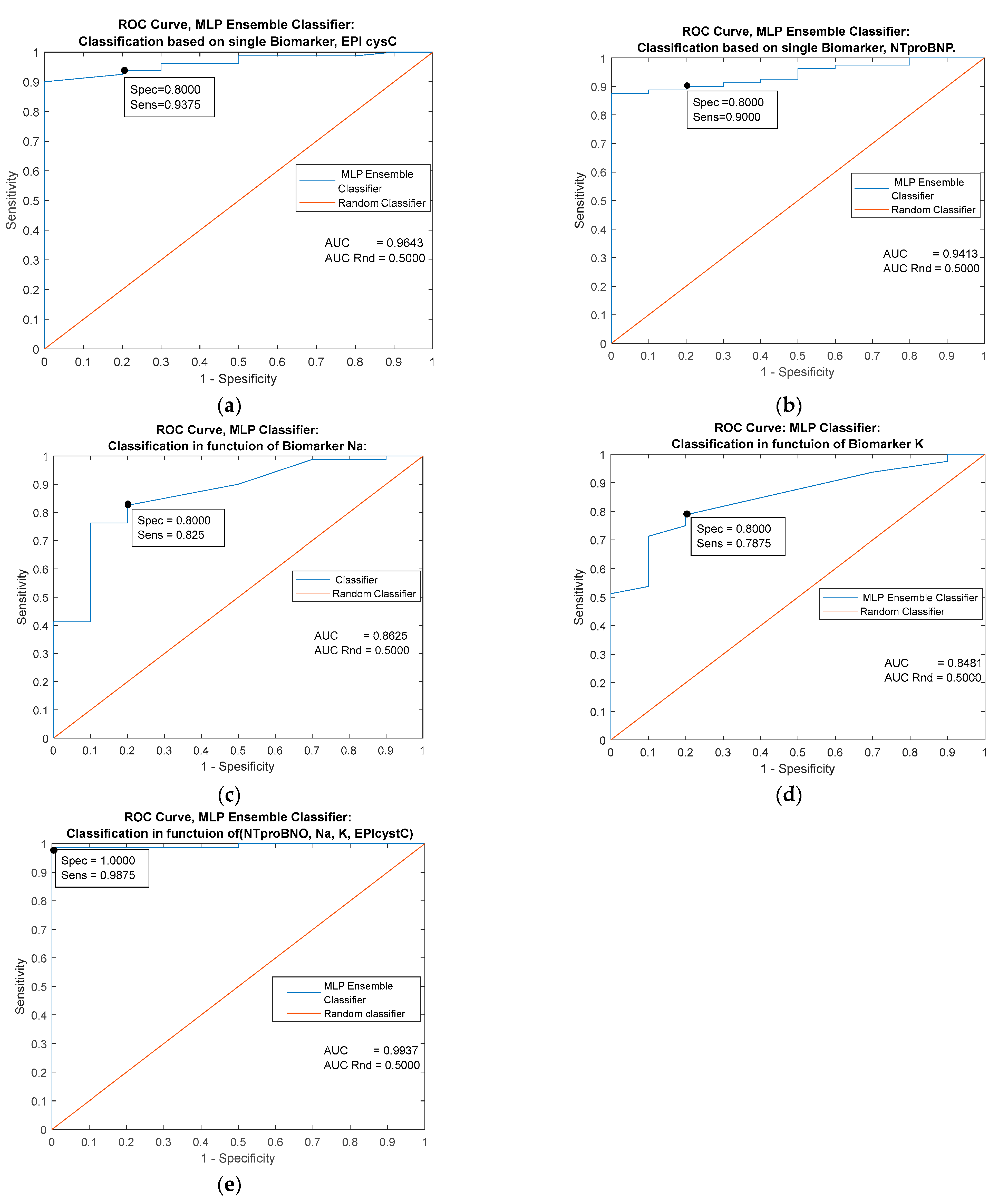
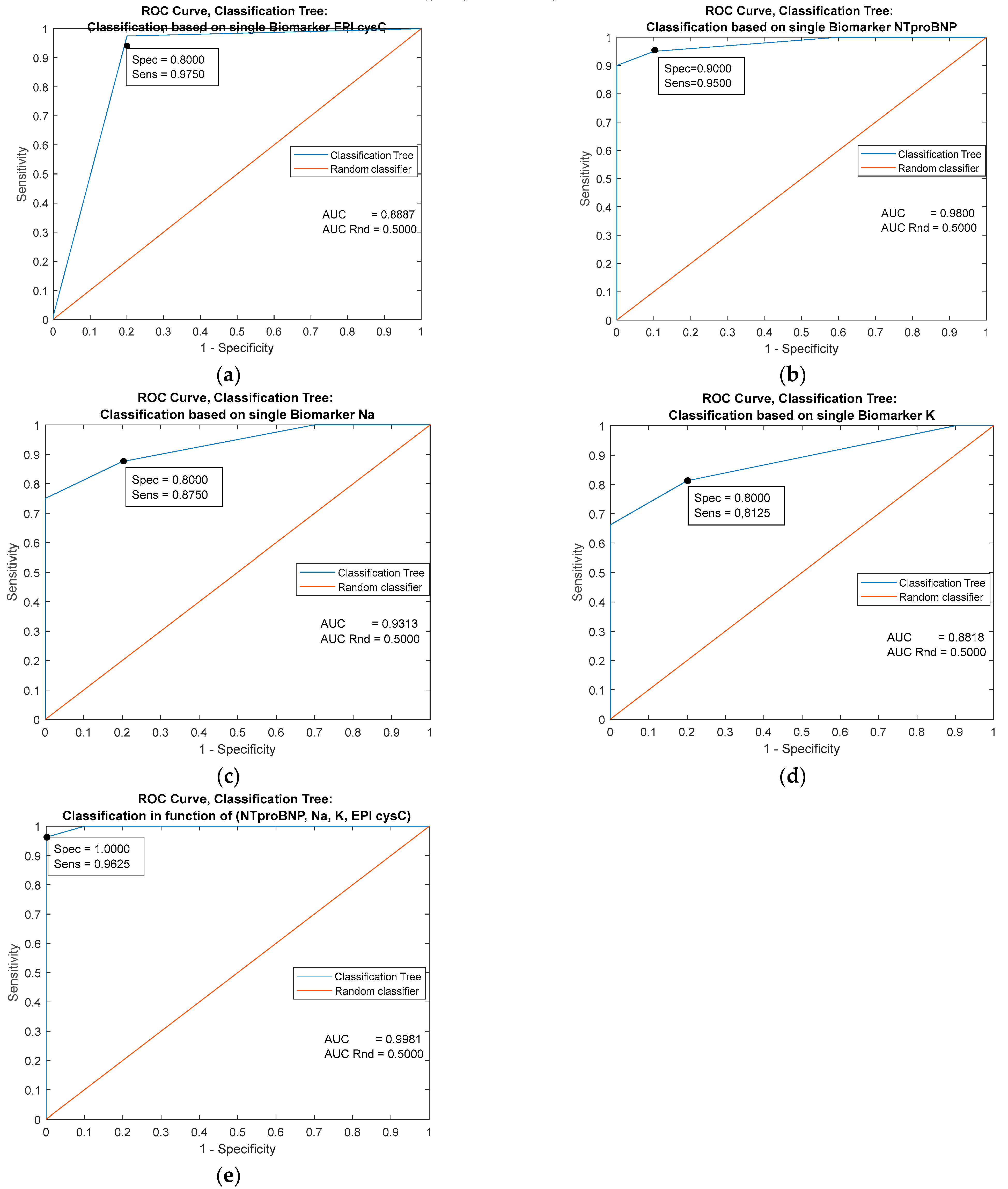
| Classifiers/ Metrics | Cutoff = 116.000 | MLP Ensemble | k-NN Ensemble | Naive Bayes | Logistic Regression | Decision trees |
| AUC | 0.9094 | 0.9643 | 0.9556 | 0.9556 | 0.9094 | 0.8887 |
| Specificity | 0.9625 | 0.9626 | 0.8000 | 0.8000 | 0.8000 | 0.9000 |
| Sensitivity | 0.8000 | 0.8000 | 0.9375 | 0.9375 | 09125 | 0.9750 |
| Youden’s index | 0.7625 | 0.7626 | 0.7375 | 0.7375 | 0.7125 | 0.8750 |
| Predictor | Single Biomarker: NTproBNP (pg/mL) | |||||
|---|---|---|---|---|---|---|
| Classifiers/ Metrics | Cutoff = 26.000 | MLP Ensemble | k-NN Ensemble | Naive Bayes | Logistic Regression | Decision trees |
| AUC | 0.9013 | 0.9413 | 0.9406 | 0.6000 | 0.9413 | 0.9800 |
| Specificity | 0.8000 | 0.8000 | 0.8000 | 0.2000 | 0.9000 | 0.9000 |
| Sensitivity | 0.7000 | 0.9000 | 0.9000 | 1.0000 | 0.8875 | 0.9500 |
| Youden’s index | 0.5000 | 0.7000 | 0.7000 | 0.2000 | 0.7875 | 0.8500 |
| Predictor | Single Biomarker: Na (mmol/L) | |||||
|---|---|---|---|---|---|---|
| Classifiers/ Metrics | Cutoff = 138.000 | MLP Ensemble | k-NN Ensemble | Naive Bayes | Logistic Regression | Decision trees |
| AUC | 0.5663 | 0.8625 | 0.7143 | 0.5000 | 0.5663 | 0.9313 |
| Specificity | 0.6375 | 0.8000 | 0.7000 | 0.0000 | 0.5000 | 0.8000 |
| Sensitivity | 0.5000 | 0.8250 | 0.7125 | 1.0000 | 0.6375 | 0.8750 |
| Youden’s index | 0.1375 | 0.6250 | 0.4125 | 0.0000 | 1375 | 0.6750 |
| Predictor | Single Biomarker: K (mmol/L) | |||||
|---|---|---|---|---|---|---|
| Classifiers/ Metrics | Cutoff = 4.8000 | MLP Ensemble | k-NN Ensemble | Naive Bayes | Logistic Regression | Decision trees |
| AUC | 0.6244 | 0.8481 | 0.6475 | 0.5000 | 0.6244 | 0.8818 |
| Specificity | 0.5000 | 0.8000 | 0.4000 | 0.0000 | 0.5000 | 0.8000 |
| Sensitivity | 0.5625 | 0.7875 | 0.8875 | 1.0000 | 0.5625 | 0.8125 |
| Youden’s index | 0.0625 | 0.5875 | 0.2875 | 0.0000 | 0.0625 | 0.6125 |
| Predictors | Combined Biomarkers: NTproBNP (pg/mL), EPI cysC (ml/min/1.73 m2), Na (mmol/L), K (mmol/L) | ||||
|---|---|---|---|---|---|
| Classifiers/ Metrics | MLP Ensemble | k-NN Ensemble | Naive Bayes | Logistic Regression | Decision trees |
| AUC | 0.9937 | 0.9887 | 0.8187 | 0.9863 | 0.9981 |
| Specificity | 1.0000 | 1.0000 | 0.7000 | 0.9000 | 1.0000 |
| Sensitivity | 0.9875 | 0.9625 | 0.9375 | 0.9500 | 0.9625 |
| Youden’s index | 0.9875 | 0.9625 | 0.6375 | 0.8500 | 0.9625 |
10. Graphic Representation of the Performance of the Applied Classifiers
11. Discussion
12. Conclusions
Author Contributions
Funding
Institutional Review Board Statement
Informed Consent Statement
Data Availability Statement
Acknowledgments
Conflicts of Interest
References
- Hadjiphilippou, S.; Kon, S.P. Cardiorenal syndrome: Review of our current understanding. J. R. Soc. Med. 2016, 109, 12–17. [Google Scholar] [CrossRef] [PubMed] [Green Version]
- Ronco, C.; Ronco, F.; McCullough, P.A. A Call to Action to Develop Integrated Curricula in Cardiorenal Medicine. Blood Purif. 2017, 44, 251–259. [Google Scholar] [CrossRef] [PubMed]
- Levey, A.S.; Coresh, J.; Tighiouart, H.; Greene, T.; Inker, L.A. Strengths and limitations of estimated and measured GFR. Nat. Rev. Nephrol. 2019, 15, 784. [Google Scholar] [CrossRef] [PubMed] [Green Version]
- Van der Laan, S.W.; Fall, T.; Soumaré, A.; Teumer, A.; Sedaghat, S.; Baumert, J.; Zabaneh, D.; van Setten, J.; Isgum, I.; Galesloot, T.E.; et al. Cystatin C and Cardiovascular Disease: A Mendelian Randomization Study. J. Am. Coll. Cardiol. 2016, 68, 934–945. [Google Scholar] [CrossRef] [Green Version]
- Inker, L.A.; Eneanya, N.D.; Coresh, J.; Tighiouart, H.; Wang, D.; Sang, Y.; Crews, D.C.; Doria, A.; Estrella, M.M.; Froissart, M.; et al. New Creatinine- and Cystatin C–Based Equations to Estimate GFR without Race. N. Engl. J. Med. 2021, 385, 1737–1749. [Google Scholar] [CrossRef] [PubMed]
- Jonsson, A.; Viklund, I.; Jonsson, A.; Valham, F.; Bergdahl, E.; Lindmark, K.; Norberg, H. Comparison of creatinine-based methods for estimating glomerular filtration rate in patients with heart failure. ESC Heart Fail. 2020, 7, 1150–1160. [Google Scholar] [CrossRef] [PubMed]
- Rizk, D.V.; Meier, D.; Sandoval, R.M.; Chacana, T.; Reilly, E.S.; Seegmiller, J.C.; DeNoia, E.; Strickland, J.S.; Muldoon, J.; Molitoris, B.A. A Novel Method for Rapid Bedside Measurement of GFR. J. Am. Soc. Nephrol. 2018, 29, 1609–1613. [Google Scholar] [CrossRef] [Green Version]
- Molitoris, B.A.; Reilly, E.S. Quantifying Glomerular Filtration Rates in Acute Kidney Injury: A Requirement for Translational Success. Semin. Nephrol. 2016, 36, 31–41. [Google Scholar] [CrossRef] [Green Version]
- Inker, L.A.; Eckfeldt, J.; Levey, A.S.; Leiendecker-Foster, C.; Rynders, G.; Manzi, J.; Waheed, S.; Coresh, J. Expressing the CKD-EPI (Chronic Kidney Disease Epidemiology Collaboration) Cystatin C Equations for Estimating GFR With Standardized Serum Cystatin C Values. Am. J. Kidney Dis. 2011, 58, 682–684. [Google Scholar] [CrossRef] [Green Version]
- Inker, L.A.; Schmid, C.H.; Tighiouart, H.; Eckfeldt, J.H.; Feldman, H.I.; Greene, T.; Kusek, J.W.; Manzi, J.; Van Lente, F.; Zhang, Y.L.; et al. Estimating glomerular filtration rate from serum creatinine and cystatin C. N. Engl. J. Med. 2012, 367, 20–29. [Google Scholar] [CrossRef] [Green Version]
- Kervella, D.; Lemoine, S.; Sens, F.; Dubourg, L.; Sebbag, L.; Guebre-Egziabher, F.; Bonnefoy, E.; Juillard, L. Cystatin C Versus Creatinine for GFR Estimation in CKD Due to Heart Failure. Am. J. Kidney Dis. 2017, 69, 321–323. [Google Scholar] [CrossRef] [Green Version]
- Ishigo, T.; Katano, S.; Yano, T.; Kouzu, H.; Ohori, K.; Nakata, H.; Nonoyama, M.; Inoue, T.; Takamura, Y.; Nagaoka, R.; et al. Overestimation of glomerular filtration rate by creatinine-based equation in heart failure patients is predicted by a novel scoring system. Geriatr. Gerontol. Int. 2020, 20, 752–758. [Google Scholar] [CrossRef] [PubMed]
- Helmersson-Karlqvist, J.; Ärnlöv, J.; Larsson, A. Cystatin C-based glomerular filtration rate associates more closely with mortality than creatinine-based or combined glomerular filtration rate equations in unselected patients. Eur. J. Prev. Cardiol. 2016, 23, 1649–1657. [Google Scholar] [CrossRef]
- National Kidney Foundation. KDOQI Clinical Practice Guideline for Diabetes and CKD: 2012 Update. Am. J. Kidney Dis. 2012, 60, 850–886. [Google Scholar] [CrossRef]
- Szummer, K.; Evans, M.; Carrero, J.J.; Alehagen, U.; Dahlstrom, U.; Benson, L.; Lund, H.L. Comparison of the Chronic Kidney Disease Epidemiology Collaboration, the Modification of Diet in Renal Disease study and the Cockcroft-Gault equation in patients with heart failure. Open Heart 2017, 4, 1–9. [Google Scholar] [CrossRef]
- Breidthardt, T.; Sabti, Z.; Ziller, R.; Rassouli, F.; Twerenbold, R.; Kozhuharov, N.; Gayat, E.; Shrestha, S.; Barata, S.; Badertscher, P.; et al. Diagnostic and prognostic value of cystatin C in acute heart failure. Clin. Biochem. 2017, 50, 1007–1013. [Google Scholar] [CrossRef]
- Di Lullo, L.; Bellasi, A.; Barbera, V.; Russo, D.; Russo, L.; Di Iorio, B.; Cozzolino, M.; Ronco, C. Pathophysiology of the cardio-renal syndromes types 1–5: An uptodate. Indian Heart J. 2017, 69, 255–265. [Google Scholar] [CrossRef]
- Taylor, C.J.; Lay-Flurrie, S.L.; Ordóñez-Mena, J.M.; Goyder, C.R.; Jones, N.R.; Roalfe, A.K.; Hobbs, F.R. Natriuretic peptide level at heart failure diagnosis and risk of hospitalisation and death in England 2004–2018. Heart 2021, 108, 543–549. [Google Scholar] [CrossRef]
- Thind, G.S.; Loehrke, M.; Wilt, J.L. Acute cardiorenal syndrome: Mechanisms and clinical implications. Clevel. Clin. J. Med. 2018, 85, 231–239. [Google Scholar] [CrossRef] [PubMed] [Green Version]
- Fan, P.-C.; Chang, C.-H.; Chen, Y.-C. Biomarkers for acute cardiorenal syndrome. Nephrology 2018, 23, 68–71. [Google Scholar] [CrossRef] [PubMed] [Green Version]
- Ruocco, G.; Palazzuoli, A.; ter Maaten, M.J. The role of the kidney in acute and chronic heart failure. Heart Fail Rev. 2019, 25, 107–118. [Google Scholar] [CrossRef]
- Herzog, C.A. Congestive Heart Failure and Chronic Kidney Disease. J. Am. Coll. Cardiol. 2019, 73, 2701–2704. [Google Scholar] [CrossRef] [PubMed]
- Rangaswami, J.; Bhalla, V.; Blair, J.E.; Chang, T.I.; Costa, S.; Lentine, K.L.; Lerma, E.V.; Mezue, K.; Molitch, M.; Mullens, W.; et al. Cardiorenal Syndrome: Classification, Pathophysiology, Diagnosis, and Treatment Strategies: A Scientific Statement From the American Heart Association. Circulation 2019, 139, e840–e878. [Google Scholar] [CrossRef]
- Naumovic, R.; Furuncic, D.; Jovanovic, D.; Stosovic, M.; Basta-Jovanovic, G.; Lezaic, V. Application of artificial neural networks in estimating predictive factors and therapeutic efficacy in idiopathic membranous nephropathy. Biomed. Pharmacother. 2010, 64, 633–638. [Google Scholar] [CrossRef] [PubMed]
- Keller, T.; Bitterlich, N.; Hilfenhaus, S.; Bigl, H.; Löser, T.; Leonhardt, P. Tumour markers in the diagnosis of bronchial carcinoma: New options using fuzzy logic-based tumour marker profiles. J. Cancer Res. Clin. Oncol. 1998, 124, 565–574. [Google Scholar] [CrossRef] [PubMed]
- Sanchez, E. Solutions in composite fuzzy relation equations: Application to medical diagnosis in brouwerian logic. In Readings in Fuzzy Sets for Intelligent Systems; Didier, D., Henri, P., Ronald, R.Y., Eds.; Morgan Kaufmann: Burlington, MA, USA, 1993; Volume 9781483214504, pp. 159–165. [Google Scholar] [CrossRef]
- Sanchez, E. Fuzzy logic and inflammatory protein variations. Clin. Chim. Acta 1998, 270, 31–42. [Google Scholar] [CrossRef] [PubMed]
- Furundzic, D.; Stankovic, S.; Jovicic, S.; Punisic, S.; Subotic, M. Distance based resampling of imbalanced classes: With an application example of speech quality assessment. Eng. Appl. Artif. Intell. 2017, 64, 440–461. [Google Scholar] [CrossRef]
- Zadeh, L.A. Fuzzy sets. Inf. Control 1965, 8, 338–353. [Google Scholar] [CrossRef] [Green Version]
- Available online: http://archive.ics.uci.edu/ml/index.php (accessed on 24 September 2022).
- Available online: http://www.kidney.org/professionals/KDOQI/gfr_calculator (accessed on 24 September 2022).
- Lippmann, R. Pattern classification using neural networks. IEEE Commun. Mag. 1989, 11, 47–64. [Google Scholar] [CrossRef]
- Guo, H.; Viktor, H.L. Learning from imbalanced data sets with boosting and data generation: The DataBoost-IM Approach. ACM SIGKDD Explor. Newsl. 2004, 6, 30–39. [Google Scholar] [CrossRef]
- Kubat, M.; Holte, R.C.; Matwin, S. Machine Learning for the Detection of Oil Spills in Satellite Radar Images. Mach. Learn. 1998, 30, 195–215. [Google Scholar] [CrossRef] [Green Version]
- Fawcett, T. An Introduction to ROC analysis. Pattern Recogn. Lett. 2006, 27, 861–874. [Google Scholar] [CrossRef]
- Provost, F.; Fawcett, T. Analysis and Visualization of Classifier Performance: Comparison Under Imprecise Class and Cost Distributions. In Proceedings of the 3rd International Conference on Knowledge Representation and Data Mining, (KDD97) Cambridge, Newport Beach, CA, USA, 14–17 August 1997; AAAI Press: Menlo Park, CA, USA, 1997; pp. 43–48. [Google Scholar]
- Maloof, M. Learning when data sets are imbalanced and when costs are unequal and unknown. In Workshop on Learning from Imbalanced Data Sets II; ICML: Washington, DC, USA, 2003; Available online: http://www.site.uottawa.ca/~nat/Workshop2003/workshop2003.html (accessed on 16 February 2023).
- Rumelhart, D.E.; Hinton, G.E.; Williams, R.J. Learning representations by back-propagating errors. Nature 1986, 323, 533–536. [Google Scholar] [CrossRef]
- Mavrakanas, T.A.; Khattak, A.; Singh, K.; Charytan, D.M. Epidemiology and Natural History of the Cardiorenal Syndromes in a Cohort with Echocardiography. Clin. J. Am. Soc. Nephrol. 2017, 12, 1624–1633. [Google Scholar] [CrossRef] [Green Version]
- Ahmad, T.; Jackson, K.; Rao, V.S.; Tang, W.W.; Brisco-Bacik, M.A.; Chen, H.H.; Felker, G.M.; Hernandez, A.F.; O’Connor, C.M.; Sabbisetti, V.S.; et al. Worsening Renal Function in Patients With Acute Heart Failure Undergoing Aggressive Diuresis Is Not Associated With Tubular Injury. Circulation 2018, 137, 2016–2028. [Google Scholar] [CrossRef]
- Wang, K.; Kestenbaum, B. Proximal Tubular Secretory Clearance. Clin. J. Am. Soc. Nephrol. 2018, 13, 1291–1296. [Google Scholar] [CrossRef] [PubMed] [Green Version]
- Kanjanahattakij, N.; Sirinvaravong, N.; Aguilar, F.; Agrawal, A.; Krishnamoorthy, P.; Gupta, S. High Right Ventricular Stroke Work Index Is Associated with Worse Kidney Function in Patients with Heart Failure with Preserved Ejection Fraction. Cardiorenal Med. 2018, 8, 123–129. [Google Scholar] [CrossRef]
- Kalmanson, D.; Stegall, H. Cardiovascular investigations and fuzzy sets theory. Am. J. Cardiol. 1975, 35, 80–84. [Google Scholar] [CrossRef]
- Pastural-Thaunat, M.; Ecochard, R.; Boumendjel, N.; Abdullah, E.; Cardozo, C.; Lenz, A.; M’Pio, I.; Szelag, J.; Fouque, D.; Walid, A.; et al. Relative Change in NT-proBNP Level: An Important Risk Predictor of Cardiovascular Congestion in Haemodialysis Patients. Nephron Extra 2012, 2, 311–318. [Google Scholar] [CrossRef]
- Rau, G.; Becker, K.; Kaufmann, R.; Zimmermann, H.-J. Fuzzy Logic and Control: Principal Approach and Potential Applications in Medicine. Artif. Organs 1995, 19, 105–112. [Google Scholar] [CrossRef]
- Levey, A.S.; Coresh, J.; Tighiouart, H.; Greene, T.; Inker, L.A. Measured and estimated glomerular filtration rate: Current status and future directions. Nat. Rev. Nephrol. 2020, 16, 51–64. [Google Scholar] [CrossRef]
- Agah, A. Introduction to Medical Applications of Artificial intelligence. In Medical Applications of Artificial Intelligence; CRC Press: Boca Raton, FL, USA; Taylor & Francis: Boca Raton, FL, USA, 2013; Chapter 1. [Google Scholar] [CrossRef]
- Tomašev, N.; Glorot, X.; Rae, J.W.; Zielinski, M.; Askham, H.; Saraiva, A.; Mottram, A.; Meyer, C.; Ravuri, S.; Protsyuk, I.; et al. A clinically applicable approach to continuous prediction of future acute kidney injury. Nature 2019, 572, 116–119. [Google Scholar] [CrossRef] [PubMed]
- Mohamadlou, H.; Lynn-Palevsky, A.; Barton, C.; Chettipally, U.; Shieh, L.; Calvert, J.; Saber, N.R.; Das, R. Prediction of Acute Kidney Injury With a Machine Learning Algorithm Using Electronic Health Record Data. Can. J. Kidney Health Dis. 2018, 5, 2054358118776326. [Google Scholar] [CrossRef] [PubMed] [Green Version]
- Zhang, Z.; Ho, K.M.; Hong, Y. Machine learning for the prediction of volume responsiveness in patients with oliguric acute kidney injury in critical care. Crit. Care 2019, 23, 1–10. [Google Scholar] [CrossRef] [Green Version]
- Griffin, M.; Rao, V.S.; Fleming, J.; Raghavendra, P.; Turner, J.; Mahoney, D.; Wettersten, N.; Maisel, A.; Ivey-Miranda, J.B.; Inker, L.; et al. Effect on Survival of Concurrent Hemoconcentration and Increase in Creatinine During Treatment of Acute Decompensated Heart Failure. Am. J. Cardiol. 2019, 124, 1707–1711. [Google Scholar] [CrossRef] [PubMed]
- May, M. Eight ways machine learning is assisting medicine. Nat. Med. 2021, 27, 2–3. [Google Scholar] [CrossRef]
- Sidey-Gibbons, A.M.J.; Sidey-Gibbons, C.J. Machine learning in medicine:a practical introduction. BMC Med. Res. Methodol. 2019, 19, 64. [Google Scholar] [CrossRef] [Green Version]
- Jordan, M.I.; Mitchell, T.M. Machine learning: Trends, perspectives, and prospects. Science 2015, 349, 255–260. [Google Scholar] [CrossRef]
- Ong, M.-S.; Magrabi, F.; Coiera, E. Automated identification of extreme-risk events in clinical incident reports. J. Am. Med. Inform. Assoc. 2012, 19, e110–e118. [Google Scholar] [CrossRef] [Green Version]
- Darcy, A.M.; Louie, A.K.; Roberts, L.W. Machine Learning and the Profession of Medicine. J. Am. Med. Assoc. 2016, 315, 551–552. [Google Scholar] [CrossRef]
- Geman, S.; Bienenstock, E.; Doursat, R. Neural Networks and the Bias/Variance Dilemma. Neural Comput. 1992, 4, 1–58. [Google Scholar] [CrossRef]
- Antoniou, T.; Mamdani, M. Evaluation of machine learning solutions in medicine. CMAJ 2021, 193, E1425–E1429. [Google Scholar] [CrossRef] [PubMed]
- Valentini, G.; Dietterich, T.G. Bias-variance analysis of support vector machines for the development of SVM-based ensemble methods. J. Machine Learning Res. 2004, 5, 725–775. [Google Scholar]
- Liu, Y.; Chen, P.-H.C.; Krause, J.; Peng, L. How to Read Articles That Use Machine Learning: Users’ guides to the medical literature. JAMA 2019, 322, 1806–1816. [Google Scholar] [CrossRef]
- Ma, B.; Wei, Q.; Chen, G. A combined measure for representative information retrieval in enterprise information systems. J. Enterp. Inf. Manag. 2011, 24, 310–321. [Google Scholar] [CrossRef]
- Bertino, S. A Measure of Representativeness of a Sample for Inferential Purposes. Int. Stat. Rev. 2006, 74, 149–159. [Google Scholar] [CrossRef]
- Kuncheva, L.; Whitaker, C.J. Measures of Diversity in Classifier Ensembles and Their Relationship with the Ensemble Accuracy. Mach. Learn. 2003, 51, 181–207. [Google Scholar] [CrossRef]
- Bian, Y.; Chen, H. When Does Diversity Help Generalization in Classification Ensembles? IEEE Trans. Cybern. 2021, 52, 9059–9075. [Google Scholar] [CrossRef]
- Etchells, E.; Ho, M.; Shojania, K.G. Value of small sample sizes in rapid-cycle quality improvement projects. BMJ Qual. Saf. 2016, 25, 202–206. [Google Scholar] [CrossRef]
- Weiskopf, N.G.; Weng, C. Methods and dimensions of electronic health record data quality assessment: Enabling reuse for clinical research. J. Am. Med. Inform. Assoc. 2013, 20, 144–151. [Google Scholar] [CrossRef] [Green Version]
- Topol, E.J. High-performance medicine: The convergence of human and artificial intelligence. Nat. Med. 2019, 25, 44–56. [Google Scholar] [CrossRef] [PubMed]
- Damman, K.; Tesani, J.M. The kidney in heart failure:an update. Eur. Heart J. 2015, 36, 1437–1444. [Google Scholar] [CrossRef] [PubMed] [Green Version]
- Ronco, C.; Di Lullo, L. Cardiorenal Syndrome in Western Countries: Epidemiology, Diagnosis and Management Approaches. Kidney Dis. 2016, 2, 151–163. [Google Scholar] [CrossRef]
- Damman, K.; Tang, W.W.; Testani, J.M.; Mcmurray, J. Terminology and definition of changes renal function in heart failure. Eur. Heart J. 2014, 35, 3413–3416. [Google Scholar] [CrossRef] [Green Version]
- Brisco, M.A.; Zile, M.; Hanberg, J.S.; Wilson, F.; Parikh, C.; Coca, S.; Tang, W.W.; Testani, J.M. Relevance of Changes in Serum Creatinine During a Heart Failure Trial of Decongestive Strategies: Insights From the DOSE Trial. J. Card. Fail. 2016, 22, 753–760. [Google Scholar] [CrossRef] [PubMed] [Green Version]
- Testani, J.M.; Kimmel, S.E.; Dries, D.L.; Coca, S.G. Prognostic Importance of Early Worsening Renal Function After Initiation of Angiotensin-Converting Enzyme Inhibitor Therapy in Patients With Cardiac Dysfunction. Circ. Heart Fail. 2011, 4, 685–691. [Google Scholar] [CrossRef] [Green Version]
- Beldhuis, I.E.; Streng, K.W.; Ter Maaten, J.M.; Voors, A.A.; van der Meer, P.; Rossignol, P.; Mcmurray, J.; Damman, K. Renin–Angiotensin System Inhibition, Worsening Renal Function, and Outcome in Heart Failure Patients With Reduced and Preserved Ejection Fraction: A meta-analysis of published study data. Circ. Heart Fail. 2017, 10, 003588. [Google Scholar] [CrossRef]
- Pfeffer, M.A.; Claggett, B.; Assmann, S.F.; Boineau, R.; Anand, I.; Clausell, N.; Desai, A.S.; Diaz, R.; Fleg, J.L.; Gordeev, I.; et al. Regional Variation in Patients and Outcomes in the Treatment of Preserved Cardiac Function Heart Failure With an Aldosterone Antagonist (TOPCAT) Trial. Circulation 2015, 131, 34–42. [Google Scholar] [CrossRef] [Green Version]
- Bärfacker, L.; Kuhl, A.; Hillisch, A.; Grosser, R.; Figueroa-Pérez, S.; Heckroth, H.; Nitsche, A.; Ergüden, J.-K.; Gielen-Haertwig, H.; Schlemmer, K.-H.; et al. Discovery of BAY 94-8862: A Nonsteroidal Antagonist of the Mineralocorticoid Receptor for the Treatment of Cardiorenal Diseases. Chemmedchem 2012, 7, 1385–1403. [Google Scholar] [CrossRef]
- Rossignol, P.; Girerd, N.; Bakris, G.; Vardeny, O.; Claggett, B.; McMurray, J.J.; Swedberg, K.; Krum, H.; van Veldhuisen, D.J.; Shi, H.; et al. Impact of eplerenone on cardiovascular outcomes in heart failure patients with hypokalaemia. Eur. J. Heart Fail. 2016, 19, 792–799. [Google Scholar] [CrossRef] [Green Version]
- Brisco, M.A.; Testani, J.M.; Cook, J.L. Renal dysfunction and chronic mechanical circulatory support: From ptient selection to long-term management and prognosis. Curr. Opin. Cardiol. 2016, 31, 277–286. [Google Scholar] [CrossRef]
- Feldman, D.; Pamboukian, S.V.; Teuteberg, J.J.; Birks, E.; Lietz, K.; Moore, S.A.; Morgan, J.A.; Arabia, F.; Bauman, M.E.; Buchholz, H.W.; et al. The 2013 International Society for Heart and Lung Transplantation Guidelines for mechanical circulatory support: Executive summary. J. Heart Lung Transplant. 2013, 32, 157–187. [Google Scholar] [CrossRef]


| Real Class | |||
|---|---|---|---|
| p | n | ||
| Predicted class | Y | TP (true positive) | FN (false negative) |
| N | FP (false positive) | TN (true negative) | |
| Parameters | Clinical Group | Control Group | p/Z | p |
|---|---|---|---|---|
| Age (year) | 70.72 ± 9.26 | 69.55 ± 32.01 | 1.079 | 0.286 |
| Na (mmol/L) | 137.75 ± 4.77 | 139.67 ± 0.82 | 1.513 | 0.130 |
| K (mmol/L) | 4.89 ± 0.99 | 4.27 ± 0.45 | 1.870 | 0.061 |
| EPI cystatin C (mL/min/1.73 m2) | 40.43 ± 25.15 | 105.5 ± 14.32 | 10.332 | <0.001 |
| BNP(pg/mL) | 1451.23 ± 1591.39 | 19.43 ± 9.18 | 4.890 | <0.001 |
| Cystatin C (mg/L) | 1.91 ± 0.73 | 0.50 ± 0.15 | 5.141 | <0.001 |
Disclaimer/Publisher’s Note: The statements, opinions and data contained in all publications are solely those of the individual author(s) and contributor(s) and not of MDPI and/or the editor(s). MDPI and/or the editor(s) disclaim responsibility for any injury to people or property resulting from any ideas, methods, instructions or products referred to in the content. |
© 2023 by the authors. Licensee MDPI, Basel, Switzerland. This article is an open access article distributed under the terms and conditions of the Creative Commons Attribution (CC BY) license (https://creativecommons.org/licenses/by/4.0/).
Share and Cite
Tasic, D.; Furundzic, D.; Djordjevic, K.; Galovic, S.; Dimitrijevic, Z.; Radenkovic, S. Data Analysis of Impaired Renal and Cardiac Function Using a Combination of Standard Classifiers. J. Pers. Med. 2023, 13, 437. https://doi.org/10.3390/jpm13030437
Tasic D, Furundzic D, Djordjevic K, Galovic S, Dimitrijevic Z, Radenkovic S. Data Analysis of Impaired Renal and Cardiac Function Using a Combination of Standard Classifiers. Journal of Personalized Medicine. 2023; 13(3):437. https://doi.org/10.3390/jpm13030437
Chicago/Turabian StyleTasic, Danijela, Drasko Furundzic, Katarina Djordjevic, Slobodanka Galovic, Zorica Dimitrijevic, and Sonja Radenkovic. 2023. "Data Analysis of Impaired Renal and Cardiac Function Using a Combination of Standard Classifiers" Journal of Personalized Medicine 13, no. 3: 437. https://doi.org/10.3390/jpm13030437