
Numerical Assessment of the Risk of Abnormal Endothelialization for Diverter Devices: Clinical Data Driven Numerical Study

 , ,
, ,
Abstract
:
1. Introduction
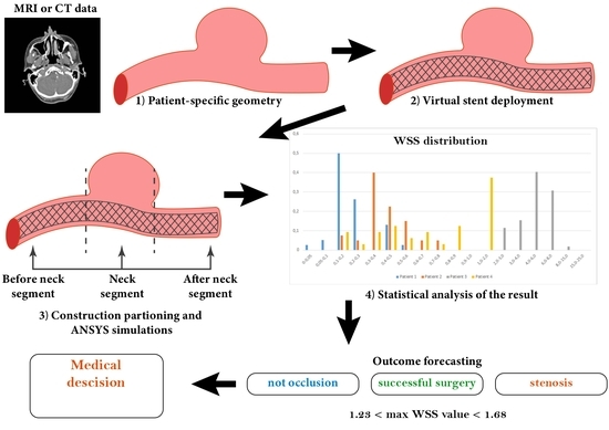
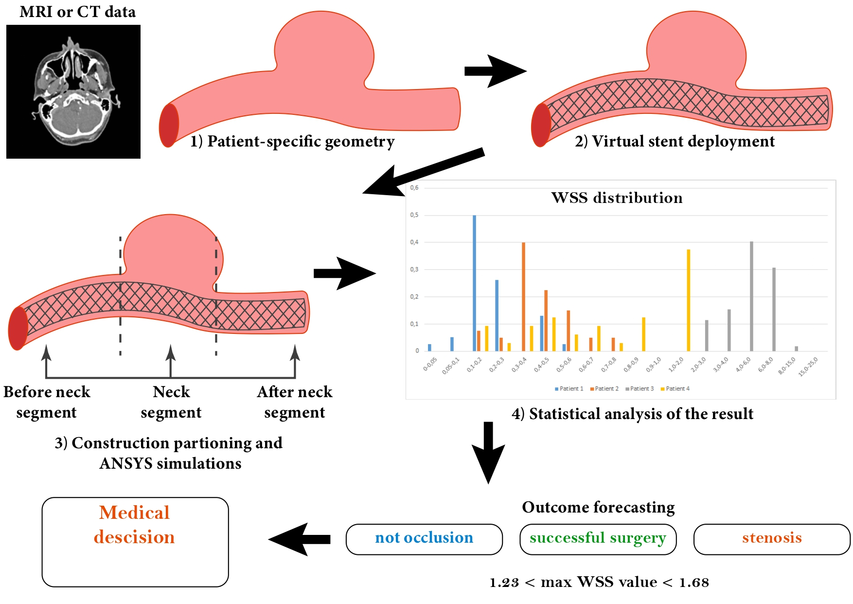
2. Materials and Methods
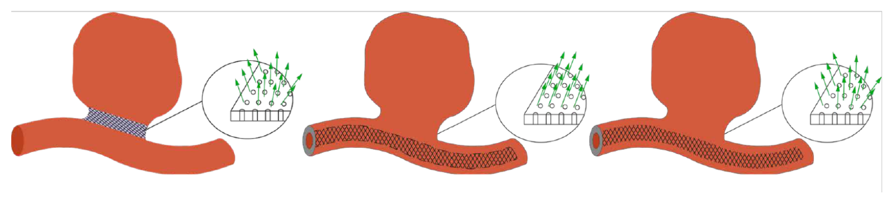
- Scenario A. The stent appears to be maximally apposed inside the vessel in such a way that its struds are pressed into the walls of the artery. In this setting, the stent interacts with the blood flow only at the orifice of the aneurysm. Thus, in this scenario, the stent looks like a layer of porous medium between the vessel body and the dome of the aneurysm;
- Scenario B. The stent is partially pressed into the vessel wall, it looks like a tube running along the center line of the vessel with a thickness of 0.8 mm [37] for patient 2 and 0.5 mm for patient 4. In this case, the tensor that determines the direction of the energy dissipation of the blood flow passing through the stent area is non-isotropic. This means that the direction is marked along the normal vector to the tube surface inside the aneurysm. This setting adequately simulates a small cell stent;
- Scenario C. This scenario is similar to scenario B without choosing the direction of energy dissipation. In this case, the tensor, which determines the direction of dissipation of the energy of the blood flow passing through the area of the stent, is isotropic. This setting corresponds to the wide-mesh stent model.
- Scenario 3.
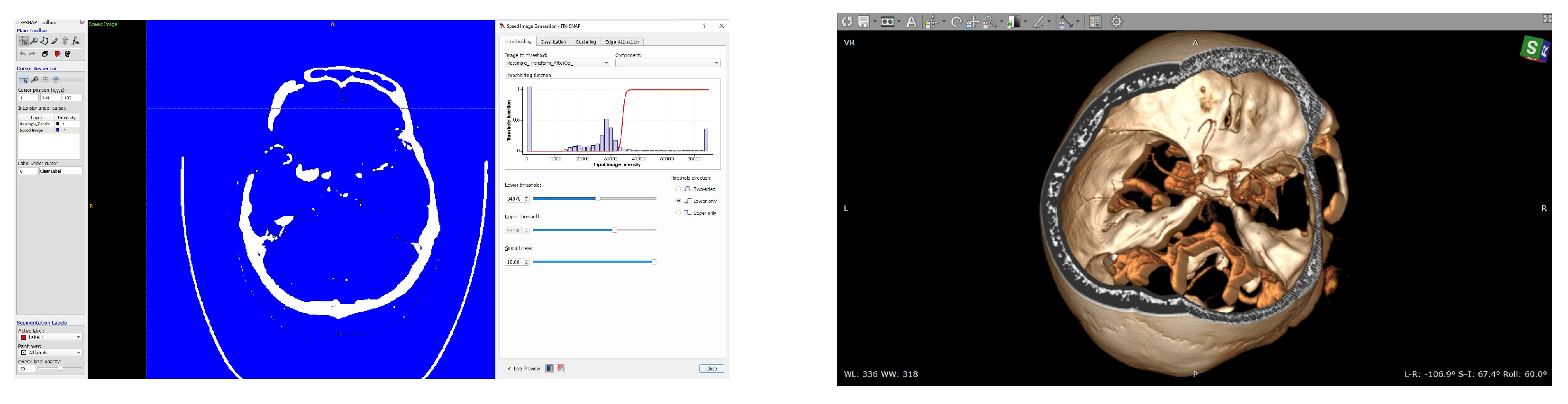
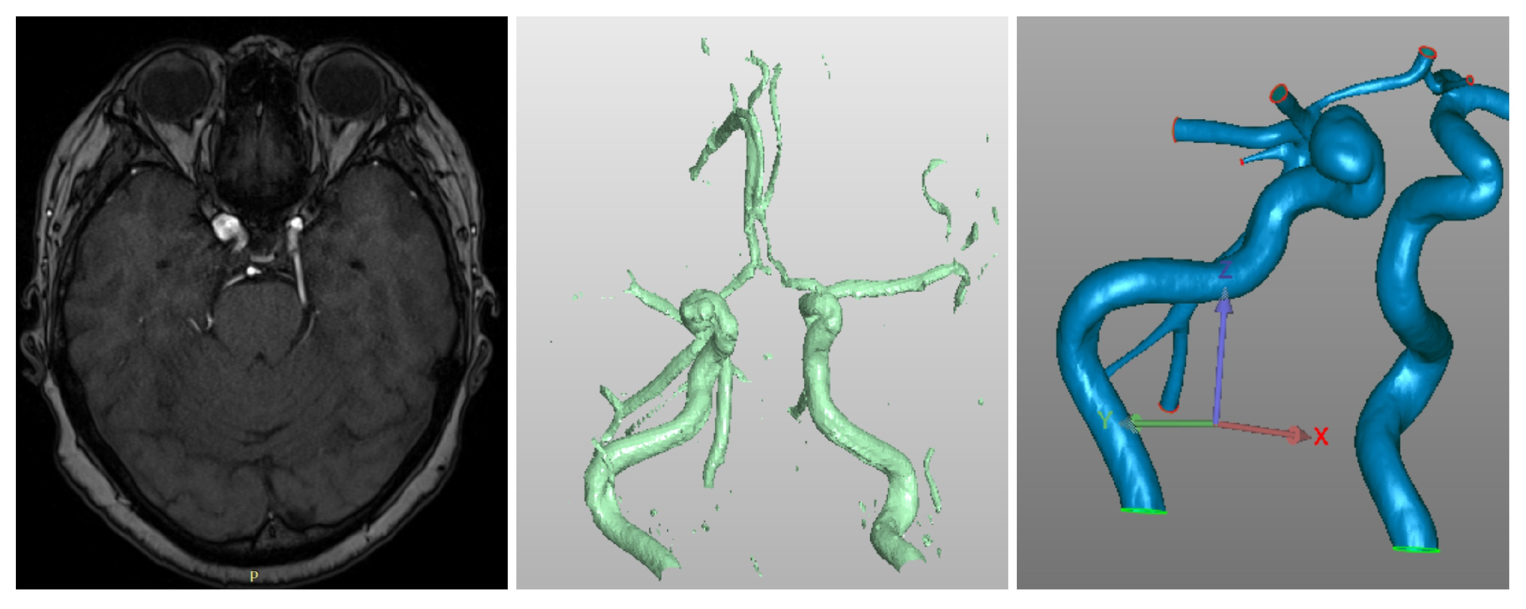
2.1. Receiving the Data
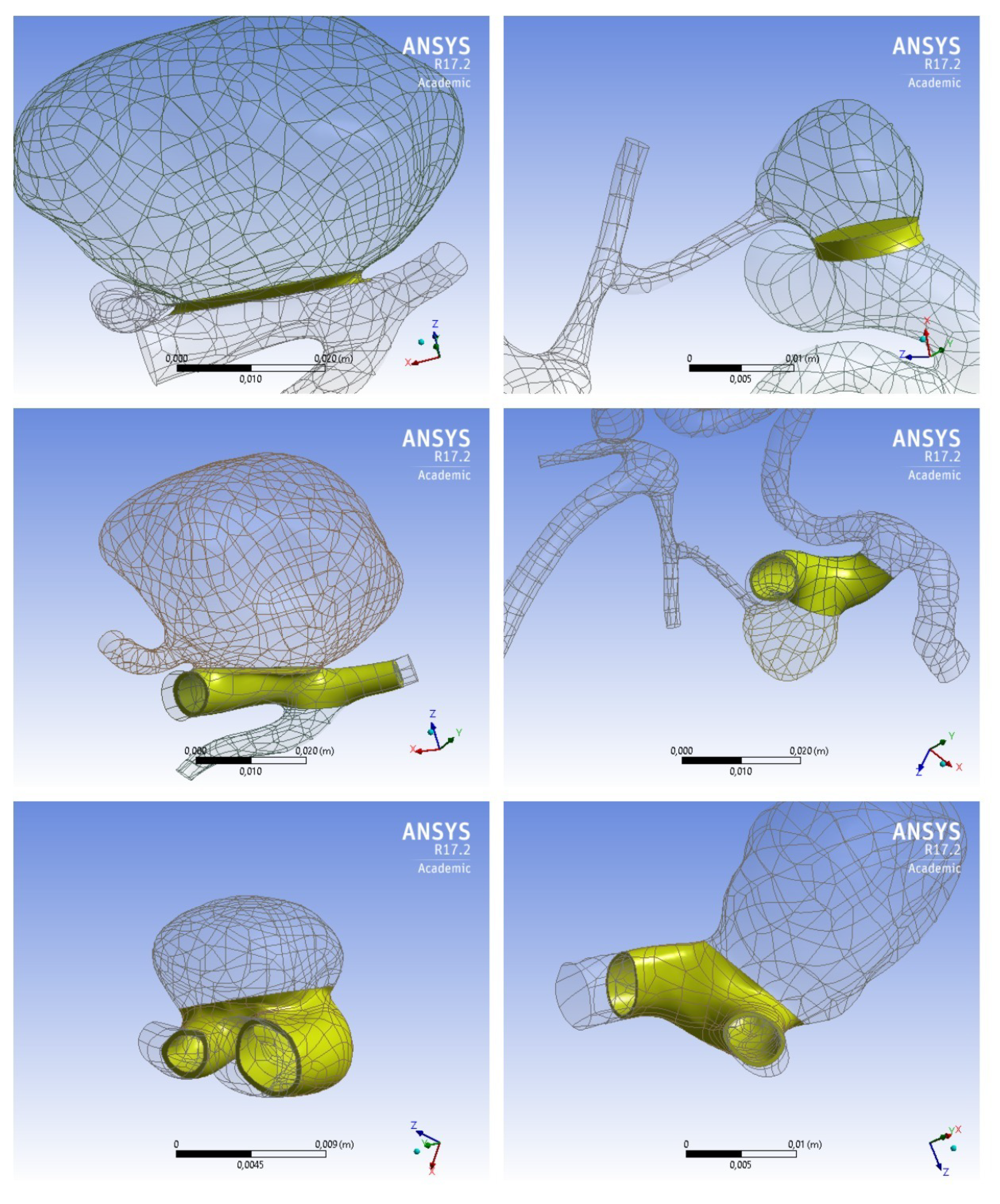
2.2. Reconstruction of Blood Vessels
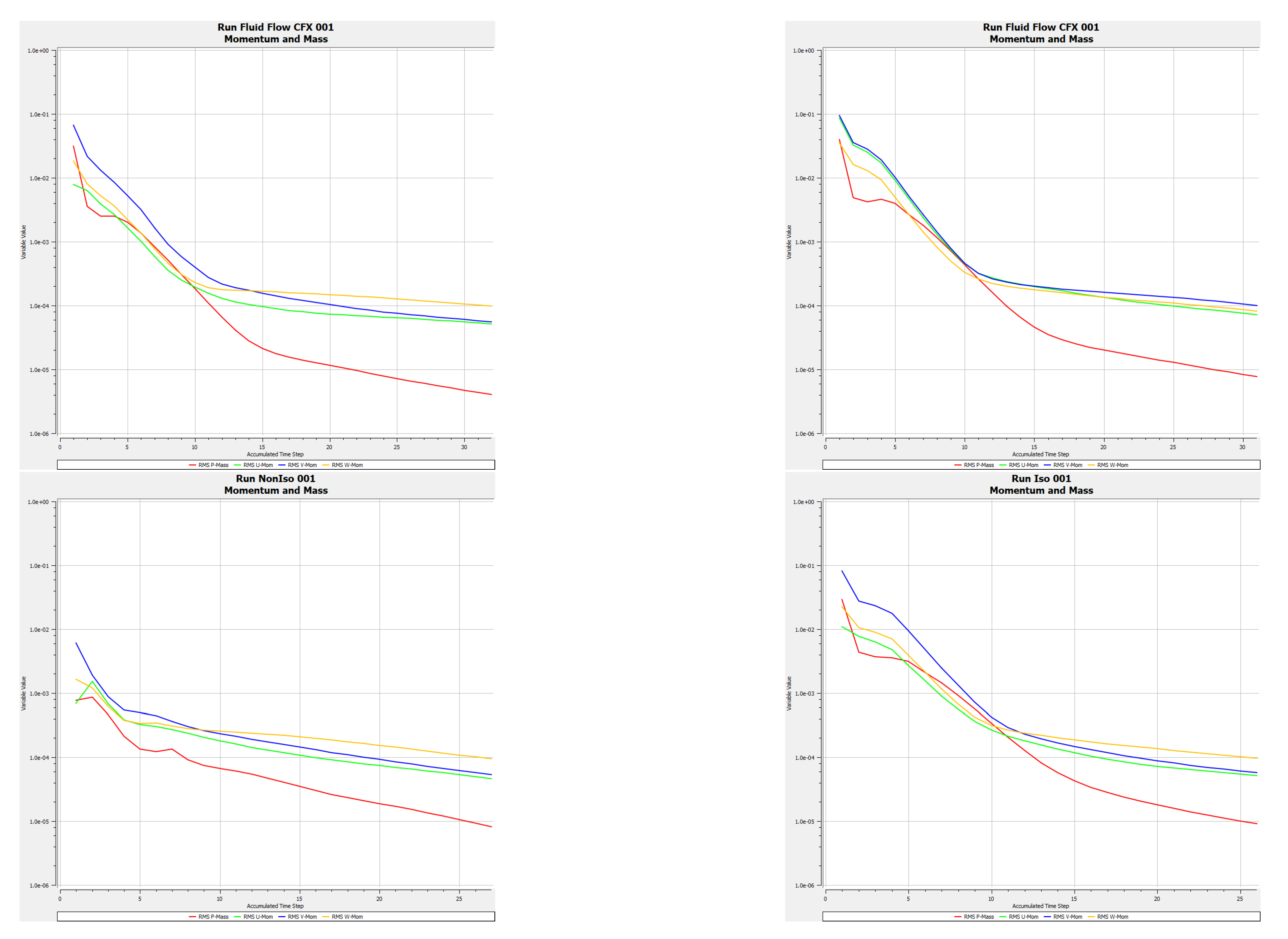
2.3. Numerical Calculations
2.4. Statistical Analysis
3. Results
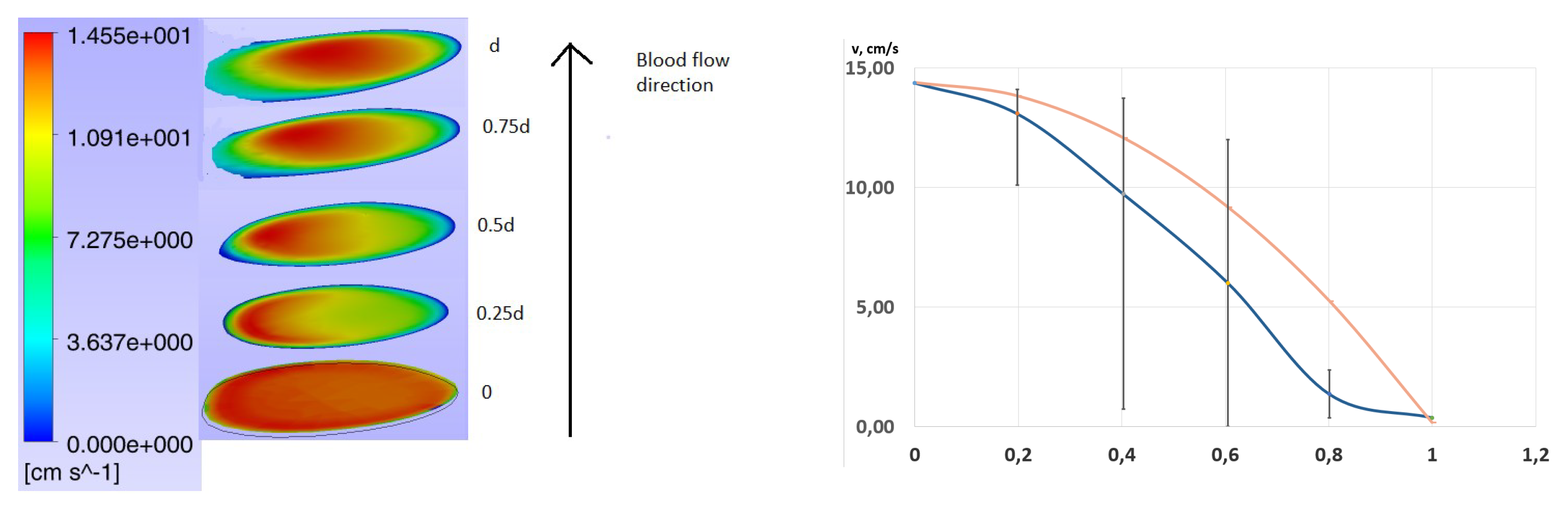
3.1. Steady Simulations
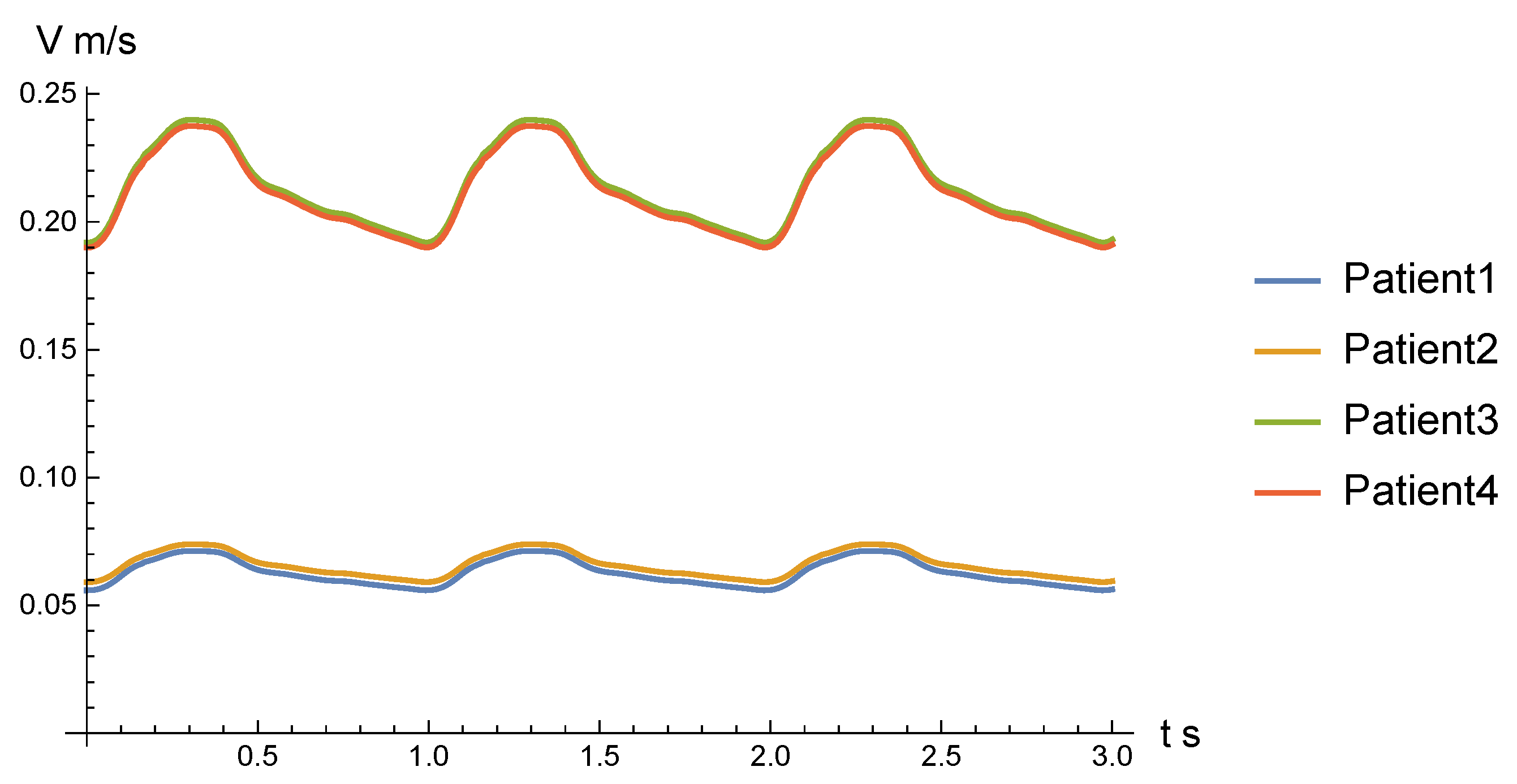
3.2. Unsteady Simulations
4. Discussion
4.1. General
4.2. Boundary Conditions
4.3. Flow-Divertion Device Design
4.4. Limitations
5. Conclusions
Supplementary Materials
Author Contributions
Funding
Institutional Review Board Statement
Informed Consent Statement
Data Availability Statement
Acknowledgments
Conflicts of Interest
Abbreviations
| WSS | Wall shear stress |
| MaxWSS | maximum value of wall shear stress in the region |
| FDD | flow diverter device |
| ICA | internal carotid artery |
| CT | computed tomography |
| MCA | middle cerebral artery |
| RSI | relative share index |
| CFD | Computational fluid dynamics |
| FSI | Fluid-structure interactions |
| LIF | Laser induced fluorescence |
Appendix A
Appendix B


Appendix C


Appendix D
References
- International Study of Unruptured Intracranial Aneurysms Investigators. Unruptured intracranial Aneurysms Risk of Rupture and Risk of surgical intervention. N. Engl. J. Med. 1998, 339, 1725–1733. [Google Scholar] [CrossRef] [PubMed]
- Rinkel, G.; Djibuti, M.; Algra, A. Prevalence and risk of rupture of intracranial aneurysms: A systematic review. Stroke 1998, 29, 251–256. [Google Scholar] [CrossRef] [PubMed] [Green Version]
- Bouhrira, N. Establishing a Mechanistic Link between Disturbed Flow and Aneurysm Formation in a 3D Cerebral Bifurcation Model. Ph.D. Thesis, Rowan University, Glassboro, NJ, USA, 2021. [Google Scholar]
- Neyazi, B.; Swiatek, V. Rupture risk assessment for multiple intracranial aneurysms: Why there is no need for dozens of clinical, morphological and hemodynamic parameters. Ther. Adv. Neurol. Disord. 2020, 13, 1756286420966159. [Google Scholar] [CrossRef] [PubMed]
- Dhar, S.; Tremmel, M.; Mocco, J.; Kim, M.; Yamamoto, J.; Siddiqui, A.; Hopkins, L.; Meng, H. Morphology parameters for intracranial aneurysm rupture risk assessment. Neurosurgery 2008, 63, 185–197. [Google Scholar] [CrossRef] [Green Version]
- Khe, A.; Chupakhin, A.; Cherevko, A.; Eliava, S.; Pilipenko, Y. Viscous dissipation energy as a risk factor in multiple cerebral aneurysms. Russ. J. Numer. Anal. Math. Model. 2015, 30, 277–287. [Google Scholar] [CrossRef]
- Ogilvy, C.; Chua, M.; Fusco, M.; Reddy, A.; Thomas, A. Stratification of recanalization for patients with endovascular treatment of intracranial aneurysms. Neurosurgery 2015, 76, 390–395. [Google Scholar] [CrossRef] [Green Version]
- van Rooij, W.; Sluzewski, M. Opinion: Imaging follow-up after coiling of intracranial aneurysms. Am. J. Neuroradiol. 2009, 30, 1646–1648. [Google Scholar] [CrossRef] [Green Version]
- Orlov, K.; Kislitsin, D.; Strelnikov, N.; Berestov, V.; Gorbatykh, A.; Shayakhmetov, T.; Seleznev, P.; Tasenko, A. Experience using pipeline embolization device with Shield Technology in a patient lacking a full postoperative dual antiplatelet therapy regimen. Intervent. Neuroradiol. 2018, 24, 270–273. [Google Scholar] [CrossRef]
- Pierot, L.; Wakhloo, A. Endovascular treatment of intracranial aneurysms. Stroke 2013, 44, 2046–2054. [Google Scholar] [CrossRef]
- Weinkauf, C.; George, E.; Zhou, W. Open versus endovascular aneurysm repair trial review. Surgery 2017, 162, 974–978. [Google Scholar] [CrossRef] [PubMed]
- Caimi, A.; Sturla, F.; Pluchinotta, F.; Giugno, L.; Secchi, F.; Votta, E.; Carminati, M.; Redaelli, A. Prediction of stenting related adverse events through patient-specific finite element modelling. J. Biomech. 2018, 79, 135–146. [Google Scholar] [CrossRef] [PubMed]
- Cebral, J.; Mut, F.; Sforza, D.; Lohner, R.; Scrivano, E.; Lylyk, P.; Putman, C. Clinical application of image-based CFD for cerebral aneurysms. Int. J. Numer. Methods Biomed. Eng. 2011, 27, 977–992. [Google Scholar] [CrossRef] [PubMed] [Green Version]
- Lv, N.; Cao, W.; Larrabide, I.; Karmonik, C.; Zhu, D.; Liu, J.; Huang, Q.; Fang, Y. Hemodynamic changes caused by multiple stenting in vertebral artery fusiform aneurysms: A patient-specific computational fluid dynamics study. Am. J. Neuroradiol. 2018, 39, 118–122. [Google Scholar] [CrossRef] [PubMed] [Green Version]
- Tanemura, H.; Ishida, F.; Miura, Y.; Umeda, Y.; Fukazawa, K.; Suzuki, H.; Sakaida, H.; Matsushima, S.; Shimosaka, S.; Taki, W. Changes in hemodynamics after placing intracranial stents. Neurol. Med. Chir. 2013, 53, 171–178. [Google Scholar] [CrossRef] [Green Version]
- Vorobtsova, N.; Yanchenko, A.; Cherevko, A.; Chupakhin, A.; Krivoshapkin, A.; Orlov, K.; Panarin, V. Modelling of cerebral aneurysm parameters under stent installation. Russ. J. Numer. Anal. Math. Model. 2013, 28, 505–516. [Google Scholar] [CrossRef]
- Tsang, A.C.; Lai, S.; Chung, W.; Tang, A.; Leung, G.; Poon, A.; Yu, A.; Chow, K. Blood flow in intracranial aneurysms treated with Pipeline embolization devices: Computational simulation and verification with Doppler ultrasonography on phantom models. Ultrasonography 2015, 34, 98–108. [Google Scholar] [CrossRef] [Green Version]
- Goubergrits, L.; Schaller, J.; Kertzscher, U.; Woelken, T.; Ringelstein, M.; Spuler, A. Hemodynamic impact of cerebral aneurysm endovascular treatment devices: Coils and flow diverters. Expert Rev. Med. Devices 2014, 11, 361–373. [Google Scholar] [CrossRef]
- Lin, N.; Brouillard, A.; Krishna, C.; Mokin, M.; Natarajan, S.; Sonig, A.; Snyder, K.; Levy, E.; Siddiqui, A. Use of coils in conjunction with the pipeline embolization device for treatment of intracranial aneurysms. Neurosurgery 2015, 76, 142–149. [Google Scholar] [CrossRef]
- Lin, N.; Brouillard, A.; Keigher, K.; Lopes, D. Utilization of pipeline embolization device for treatment of ruptured intracranial aneurysms: US multicenter experience. J. Neurointerv. Surg. 2015, 7, 808–815. [Google Scholar] [CrossRef]
- Wang, Y.; Song, S.; Zhou, G.; Liu, D.; Xia, X. Strategy of endovascular treatment for renal artery aneurysms. Clinic. Radiol. 2018, 73, 414.e1–414.e5. [Google Scholar] [CrossRef] [PubMed]
- Wang, C.; Tian, Z.; Liu, J.; Jing, L.; Paliwal, N. Hemodynamic alterations after stent implantation in 15 cases of intracranial aneurysm. Acta Neurochir. 2016, 158, 811–819. [Google Scholar] [CrossRef] [PubMed]
- Yuan, J.; Huang, C.; Li, Z. Hemodynamic Characteristics Associated with Recurrence of Middle Cerebral Artery Bifurcation Aneurysms After Total Embolization. Clin. Interv. Aging 2021, 2021, 2023–2032. [Google Scholar] [CrossRef] [PubMed]
- Frolov, S.; Sindeev, S.; Kirschke, J.; Arnold, P.; Prothmann, S. CFD and MRI studies of hemodynamic changes after flow diverter implantation in a patient-specific model of the cerebral artery. Exp. Fluids 2018, 59, 176. [Google Scholar] [CrossRef]
- Seshadhri, S.; Janiga, G. Impact of stents and flow diverters on hemodynamics in idealized aneurysm models. J. Biomech. Eng. 2011, 133, 071005. [Google Scholar] [CrossRef]
- Friesen, J.; Bergner, J.; Triess, S. Comparison of existing aneurysm models and their path forward. Comput. Methods Programs Biomed. Updat. 2021, 1, 100019. [Google Scholar] [CrossRef]
- Liu, Q.; Zhang, Y.; Yang, J.; Yang, Y.; Li, M.; Chen, S.; Jiang, P.; Wang, N.; Zhang, Y.; Liu, J.; et al. The Relationship of Morphological-Hemodynamic Characteristics, Inflammation, and Remodeling of Aneurysm Wall in Unruptured Intracranial Aneurysms. Transl. Stroke Res. 2022, 13, 88–99. [Google Scholar] [CrossRef]
- Etminan, N.; Rinkel, G. Unruptured intracranial aneurysms: Development, rupture and preventive management. Nat. Rev. Neurol. 2016, 12, 699–713. [Google Scholar] [CrossRef]
- Frosen, J.; Cebral, J. Flow-induced, inflammation-mediated arterial wall remodeling in the formation and progression of intracranial aneurysms. Neurosurg. Focus 2019, 47, E21. [Google Scholar] [CrossRef] [Green Version]
- Mach, G.; Sherif, C.; Windberger, U.; Gruber, A. A non-Newtonian model for blood flow behind a flow diverting stent. In Proceedings of the COMSOL Conference, Munich, Germany, 12–14 October 2016. [Google Scholar]
- Peach, T.; Ngoepe, M.; Spranger, K.; Zajarias-Fainsod, D.; Ventikos, Y. Personalizing flow-diverter intervention for cerebral aneurysms: From computational hemodynamics to biochemical modeling. Int. J. Numer. Methods Biomed. Eng. 2014, 30, 1387–1407. [Google Scholar] [CrossRef]
- Spranger, K.; Ventikos, Y. Which Spring is the Best? Comparison of Methods for Virtual Stenting. J. Biomed. Eng. 2014, 61, 1998–2010. [Google Scholar] [CrossRef] [PubMed]
- Chodzyǹski, K.; Uzureau, P.; Nuyens, V. The impact of arterial flow complexity on flow diverter outcomes in aneurysms. Sci. Rep. 2020, 10, 10337. [Google Scholar] [CrossRef] [PubMed]
- Li, Y.; Zhang, M.; Verrelli, D.; Chong, W.; Ohta, M.; Qian, Y. Numerical simulation of aneurysmal haemodynamics with calibrated porous-medium models of flow-diverting stents. J. Biomech. 2018, 80, 88–94. [Google Scholar] [CrossRef] [PubMed]
- Raschi, M.; Mut, F.; Lohner, R.; Cebral, J. Strategy for modeling flow diverters in cerebral aneurysms as a porous medium. Int. J. Numer. Methods Biomed. Eng. 2014, 30, 909–925. [Google Scholar] [CrossRef]
- Ren, Y.; Chen, G.; Liu, Z.; Cai, Y.; Lu, G.; Li, Z. Reproducibility of image based computational models of intracranial aneurysm: A comparison between 3D rotational angiography, CT angiography and MR angiography. Biomed. Eng. 2016, 15, 50. [Google Scholar] [CrossRef] [Green Version]
- Tang, L.; Wang, L.; Li, C.; Hu, P.; Jia, Y.; Wang, G.; Li, Y. Treatment of basilar artery stenosis with an Apollo balloon-expandable stent: A single-centre experience with 61 consecutive cases. Acta Neurol. Belg. 2020, 121, 1423–1427. [Google Scholar] [CrossRef]
- Yushkevich, P.; Piven, J.; Hazlett, H.; Smith, R.; Ho, S.; Gee, J.; Gerig, G. User-guided 3D active contour segmentation of anatomical structures: Significantly improved efficiency and reliability. Neuroimage 2006, 31, 1116–1128. [Google Scholar] [CrossRef] [Green Version]
- ANSYS. ANSYS Documentation, ANSYS CFX-Solver Theory Guide. Available online: http://www.ansys.com/ (accessed on 6 February 2022).
- Parshin, D.; Kuyanova, Y.; Kislitsin, D.; Windberger, U.; Chupakhin, A. On the Impact of Flow-Diverters on the Hemodynamics of Human Cerebral Aneurysms. J. Appl. Mech. Tech. Phys. 2018, 59, 963–970. [Google Scholar] [CrossRef]
- Oliveira, I.; Santos, G. Non-Newtonian Blood Modeling in Intracranial Aneurysm Hemodynamics: Impact on the Wall Shear Stress and Oscillatory Shear Index Metrics for Ruptured and Unruptured Cases. J. Biomech. Eng. 2021, 143, 071006. [Google Scholar] [CrossRef]
- Skiadopoulos, A.; Neofytou, P.; Housiadas, C. Comparison of blood rheological models in patient specific cardiovascular system simulations. J. Hydrodyn. 2017, 29, 293–304. [Google Scholar] [CrossRef]
- Baskurt, O.; Hardeman, M.; Rampling, M.; Meiselman, H. Handbook of Hemorheology and Hemodynamics Biomedical and Health Research; IOS Press: Amsterdam, The Netherlands, 2007. [Google Scholar]
- Khe, A.; Cherevko, A.; Chupakhin, A.; Krivoshapkin, A.; Orlov, K.; Panarin, V. Hemodynamic monitoring of cerebral vessels. J. Appl. Math Tech. Phys. 2017, 58, 7–16. (In Russian) [Google Scholar]
- Orlov, K.; Panarin, V.; Krivoshapkin, A.; Kislitsin, D.; Berestov, V.; Shayakhmetov, T. Assessment of periprocedural hemodynamic changes in arteriovenous malformation vessels by endovascular dual-sensor guidewire. Interv. Neuroradiol. 2015, 21, 101–107. [Google Scholar] [CrossRef] [PubMed] [Green Version]
- Zarrinkoob, L.; Ambarki, K.; Wåhlin, A.; Birgander, R.; Eklund, A.; Malm, J. Blood flow distribution in cerebral arteries. J. Cereb. Blood Flow Metab. 2015, 35, 648–654. [Google Scholar] [CrossRef] [Green Version]
- Nornadiah, M.; Yap, B. Power comparisons of Shapiro-Wilk, Kolmogorov-Smirnov, Lilliefors and Anderson-Darling tests. J. Stat. Model. Anal. 2011, 2, 21–33. [Google Scholar]
- Spurk, J.; Aksel, N. Fluid Mechanics; Springer: Berlin/Heidelberg, Germany, 2008. [Google Scholar]
- Ravindran, K.; Casabella, A.; Cebral, J. Mechanism of Action and Biology of Flow Diverters in the Treatment of Intracranial Aneurysms. Neurosurgery 2019, 86, S13–S19. [Google Scholar] [CrossRef] [PubMed]
- Kim, J. Hemodinamic features of microsurgically identified, thin-walled regions of unruptured middle cerebral artery aneurism characterized using computational fluid dynamics. Neurosurgery 2019, 86, 851–859. [Google Scholar] [CrossRef]
- Cebral, J.R.; Mut, F.; Weir, J.; Putman, C.M. Association of Hemodynamic Characteristics and Cerebral Aneurysm Rupture. Am. J. Neuroradiol. 2011, 32, 264–270. [Google Scholar] [CrossRef]
- Sha, L.; Chopard, B. Continuum model for flow diverting stents in 3D patient-specific simulation of intracranial aneurysms. J. Comput. Sci. 2019, 38, 101045. [Google Scholar]
- Alkhalili, K.; Hanallah, J.; Cobb, M. The Effect of Stents in Cerebral Aneurysms: A Review. Asian J. Neurosurg. 2018, 13, 201–211. [Google Scholar] [CrossRef]
- Augsburger, L.; Reymond, P. Intracranial Stents Being Modeled as a Porous Medium: Flow Simulation in Stented Cerebral Aneurysms. Ann. Biomed. Eng. 2011, 39, 850–863. [Google Scholar] [CrossRef]
- Boiko, A.; Akulov, A.; Chupahin, A. Measurement of viscous flow velocity and flow visualization using two magnetic resonance imagers. J. Appl. Mech. Tech. Phys. 2017, 58, 209–213. [Google Scholar] [CrossRef]
- Ranftl, S.; Müller, T.; Windberger, U. A Bayesian approach to blood rheological uncertaintiesin aortic hemodynamics. Int. J. Numer. Methods Biomed. Eng. 2022, e3576. [Google Scholar]
- Denner, F.; Evrad, F.; Serfaty, R. Artificial viscosity model to mitigate numerical artefacts at fluid interfaces with surface tension. Comput. Fluids 2017, 143, 59–72. [Google Scholar] [CrossRef] [Green Version]
- Cebral, J.; Mut, F.; Weir, J. Quantitative Characterization of the Hemodynamic Environment in Ruptured and Unruptured Brain Aneurysms. Am. J. Neuroradiol. 2011, 32, 145–151. [Google Scholar] [CrossRef] [PubMed] [Green Version]
- Metaxa, E.; Tremmel, M. Characterization of Critical Hemodynamics Contributing to Aneurysmal Remodeling at the Basilar Terminus in a Rabbit Model. Stroke 2010, 41, 1774–1782. [Google Scholar] [CrossRef] [PubMed] [Green Version]
- Castro, M.; Putman, C. Hemodynamic Patterns of Anterior Communicating Artery Aneurysms: A Possible Association with Rupture. Am. J. Neuroradiol. 2009, 30, 297–302. [Google Scholar] [CrossRef] [PubMed] [Green Version]
- Boussel, L.; Rayz, V.; McCulloch, C.; Martin, A.; Acevedo-Bolton, G.; Lawton, M.; Higashida, R.; Smith, W.S.; Young, W.L.; Saloner, D. Aneurysm Growth Occurs at Region of Low Wall Shear Stress: Patient-Specific Correlation of Hemodynamics and Growth in a Longitudinal Study. Stroke 2008, 39, 2997–3002. [Google Scholar] [CrossRef] [Green Version]
- Fu, F.; Wei, J.; Zhang, M.; Yu, F.; Xiao, Y.; Rong, D.; Shan, Y.; Li, Y.; Zhao, C.; Liao, F.; et al. Rapid vessel segmentation and reconstruction of head and neck angiograms using 3D convolutional neural network. Nat. Commun. 2020, 11, 4829. [Google Scholar] [CrossRef]
- Meijs, M.; Patel, A.; Prokop, M. Robust Segmentation of the Full Cerebral Vasculature in 4D CT of Suspected Stroke Patients. Sci. Rep. 2017, 7, 15622. [Google Scholar] [CrossRef] [Green Version]
- Lozovskiy, A.; Olshanskii, M.; Vassilevski, Y. Analysis and assessment of a monolithic FSI finite element method. Comput. Fluids 2019, 179, 277–288. [Google Scholar] [CrossRef]
- Tsibulskaya, E.; Lipovka, A.; Chupahin, A.; Dubovoy, A.; Parshin, D. The Relationship between the Strength Characteristics of Cerebral Aneurysm Walls with Their Status and Laser-Induced Fluorescence Data. Biomedicines 2021, 9, 537. [Google Scholar] [CrossRef] [PubMed]
- Yasuno, K.; Bakırcıoğlu, M.; Low, S.; Gaál, E.; Ruigrok, Y. Common variant near the endothelin receptor type A (EDNRA) gene is associated with intracranial aneurysm risk. Proc. Natl. Acad. Sci. USA 2011, 108, 19707–19712. [Google Scholar] [CrossRef] [PubMed] [Green Version]
- Lindgren, A.; Kurki, M.; Riihinen, A.; Koivisto, T.; Ronkainen, A. Type 2 diabetes and risk of rupture of saccular intracranial aneurysm in Eastern Finland. Diabetes Care 2013, 36, 2020–2026. [Google Scholar] [CrossRef] [PubMed] [Green Version]
- Rumbaut, R. Platelet-Vessel wall interactions in hemostasis and thrombosis. Life Sci. San Rafael 2010, 2, 1–75. [Google Scholar] [CrossRef]


| Patient 1 | Patient 2 | Patient 3 | Patient 4 | |
|---|---|---|---|---|
| Sex | w | w | w | w |
| Age | 73 | 65 | 64 | 58 |
| Aneurysm location | M1 ICA | M1 ICA | ICA | ICA |
| Status after the treatment | Success | Occlusion did not occur | In stent stenosis | In stent stenosis |
| Patients | ||||
|---|---|---|---|---|
| Patient 1 | 0.057 m/s | 0.071 m/s | 0.071 m/s | 0.06 m/s |
| Patient 2 | 0.06 m/s | 0.074 m/s | 0.074 m/s | 0.063 m/s |
| Patient 3 | 0.196 m/s | 0.239 m/s | 0.239 m/s | 0.204 m/s |
| Patient 4 | 0.191 m/s | 0.235 m/s | 0.237 m/s | 0.202 m/s |
| Modeling Scenarios | Initial Configuration without Stent | Scenario A Plug | Scenario B FDD-Tube (Non-Isotropic) | Scenario C, FDD-Tube (Isotropic) |
|---|---|---|---|---|
| Flow to the aneurysm | 1.62 | 1.34 | 1.17 | 1.18 |
| g/s | 0.39 | 0.17 | 0.13 | 0.32 |
| 4.1 | 3.6 | 3.12 | 3.13 | |
| 3.72 | 2.81 | 2.58 | 2.55 | |
| WSS | 2.37 | 3.59 | 5.34 | 5.36 |
| maximum value, Pa | 0.28 | 0.38 | 0.38 | 0.94 |
| 38.57 | 34.48 | 25.45 | 25.26 | |
| 5.23 | 2.97 | 2.13 | 2.7 | |
| Number of iterations | 7,358,495 | +200%, −8% | +200%, +33% | +200%, +33% |
| number of nodes | 5,487,579 | +700%, −1% | +200%, +53% | +200%, +53% |
| 6,366,709 | +100%, +0% | +200%, +173% | +200%, +173% | |
| 8,416,665 | +200%, +0% | +200%, +115% | +200%, +115% |
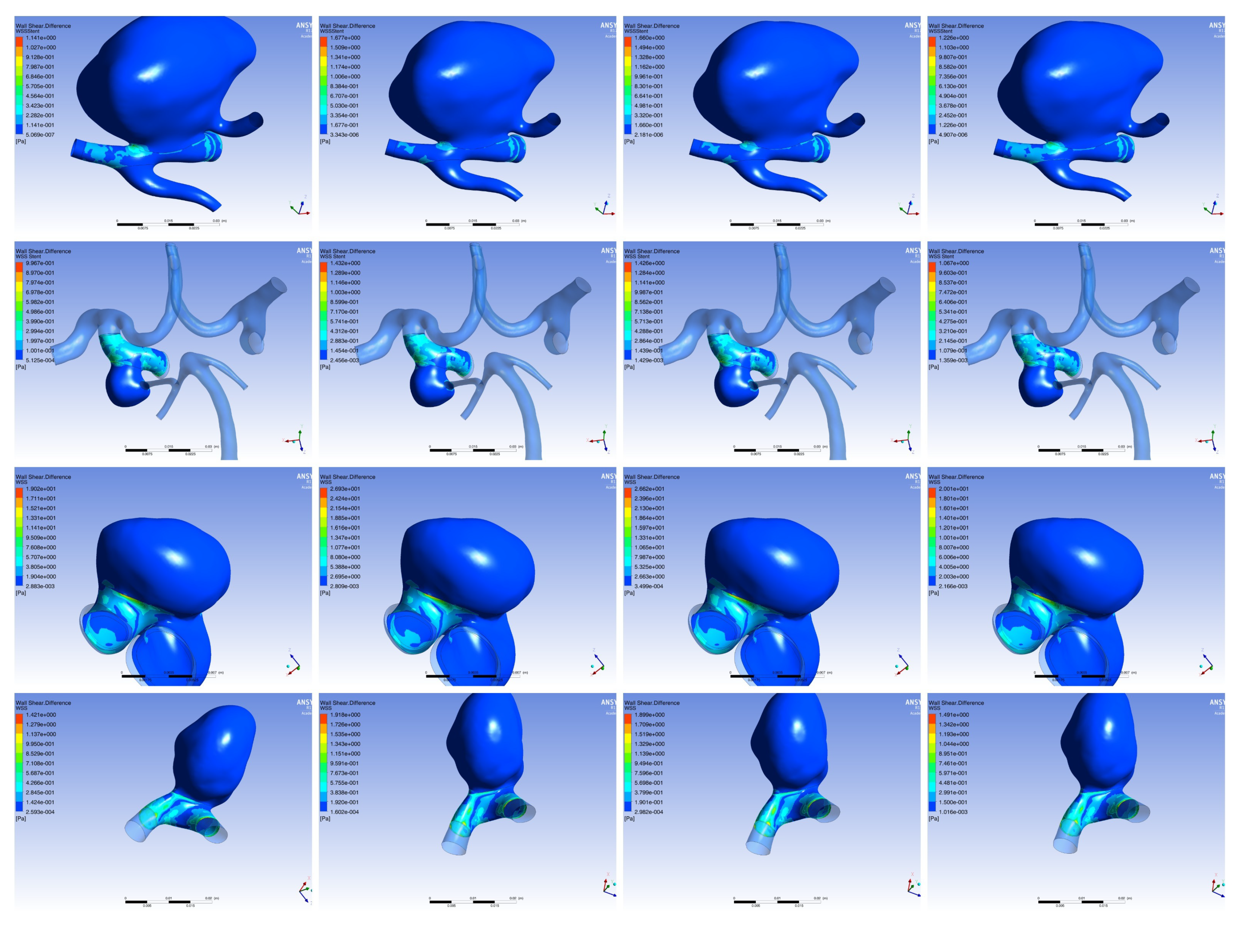
| Patients | Clinical Outcome | ||||
|---|---|---|---|---|---|
| Patient 3 | 19.02 Pa | 26.93 Pa | 26.62 Pa | 20.01 Pa | In stent stenosis |
| Patient 4 | 1.421 Pa | 1.918 Pa | 1.899 Pa | 1.491 Pa | In stent stenosis |
| Patient 1 | 1.141 Pa | 1.677 Pa | 1.660 Pa | 1.226 Pa | Norm |
| Patient 2 | 0.997 Pa | 1.432 Pa | 1.426 Pa | 1.067 Pa | No occlusion |
| Patients | Total Shear Force, N | Area, m2 | RSI, Pa | Result |
|---|---|---|---|---|
| Patient 1 | 0.00006 | 0.00071 | 0.09 | Norm |
| 0.00008 | 0.00071 | 0.109 | ||
| 0.00008 | 0.00071 | 0.113 | ||
| 0.00007 | 0.00071 | 0.098 | ||
| Patient 2 | 0.00009 | 0.00053 | 0.172 | No occlusion |
| 0.00012 | 0.00053 | 0.234 | ||
| 0.00012 | 0.00053 | 0.23 | ||
| 0.00008 | 0.00053 | 0.158 | ||
| Patient 3 | 0.00019 | 0.00018 | 1.029 | In stent stenosis |
| 0.00025 | 0.00018 | 1.385 | ||
| 0.00027 | 0.00018 | 1.466 | ||
| 0.00021 | 0.00018 | 1.146 | ||
| Patient 4 | 0.00012 | 0.00038 | 0.306 | In stent stenosis |
| 0.00015 | 0.00038 | 0.407 | ||
| 0.00016 | 0.00038 | 0.419 | ||
| 0.00013 | 0.00038 | 0.332 |
Publisher’s Note: MDPI stays neutral with regard to jurisdictional claims in published maps and institutional affiliations. |
© 2022 by the authors. Licensee MDPI, Basel, Switzerland. This article is an open access article distributed under the terms and conditions of the Creative Commons Attribution (CC BY) license (https://creativecommons.org/licenses/by/4.0/).
Share and Cite
Tikhvinskii, D.; Kuianova, J.; Kislitsin, D.; Orlov, K.; Gorbatykh, A.; Parshin, D. Numerical Assessment of the Risk of Abnormal Endothelialization for Diverter Devices: Clinical Data Driven Numerical Study. J. Pers. Med. 2022, 12, 652. https://doi.org/10.3390/jpm12040652
Tikhvinskii D, Kuianova J, Kislitsin D, Orlov K, Gorbatykh A, Parshin D. Numerical Assessment of the Risk of Abnormal Endothelialization for Diverter Devices: Clinical Data Driven Numerical Study. Journal of Personalized Medicine. 2022; 12(4):652. https://doi.org/10.3390/jpm12040652
Chicago/Turabian StyleTikhvinskii, Denis, Julia Kuianova, Dmitrii Kislitsin, Kirill Orlov, Anton Gorbatykh, and Daniil Parshin. 2022. "Numerical Assessment of the Risk of Abnormal Endothelialization for Diverter Devices: Clinical Data Driven Numerical Study" Journal of Personalized Medicine 12, no. 4: 652. https://doi.org/10.3390/jpm12040652