
Variation of the Three-Dimensional Femoral J-Curve in the Native Knee


Abstract
:1. Introduction
2. Materials and Methods
2.1. Patient Datasets
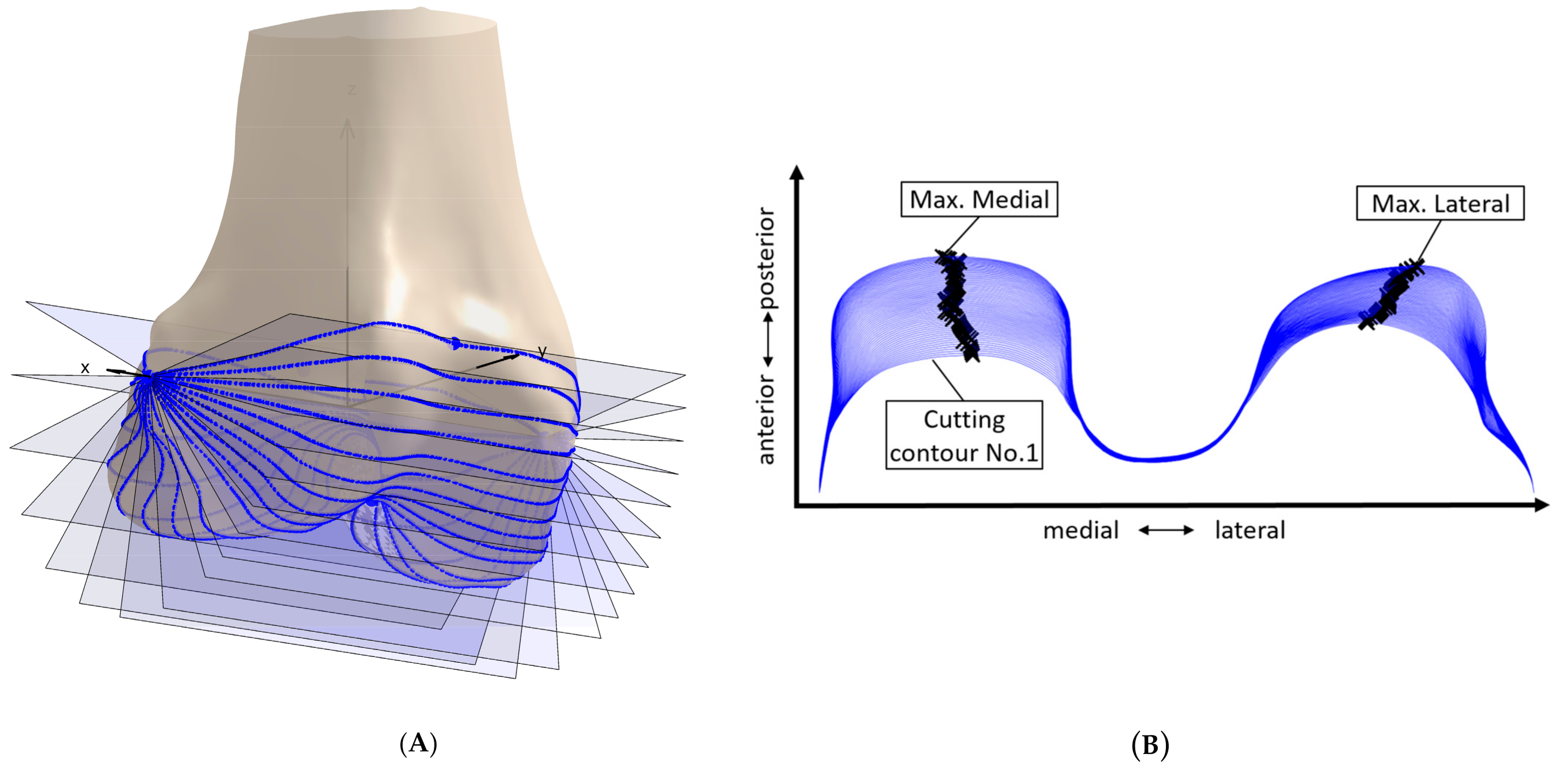
2.2. Contour Derivation
2.3. Principal Component Analysis
2.4. Geometric Parameter Analysis
3. Results
4. Discussion
Limitations
5. Conclusions
Author Contributions
Funding
Institutional Review Board Statement
Informed Consent Statement
Conflicts of Interest
References
- Klein, P.; Sommerfeld, P. Biomechanik der Menschlichen Gelenke—Biomechanik der Wirbelsäule; Nachdr. d. Aufl von 2004 in 1 Bd; Urban & Fischer in Elsevier: München, Germany, 2012; ISBN 3437552031. [Google Scholar]
- Kessler, O.; Dürselen, L.; Banks, S.; Mannel, H.; Marin, F. Sagittal curvature of total knee replacements predicts in vivo kinematics. Clin. Biomech. (Bristol Avon) 2007, 22, 52–58. [Google Scholar] [CrossRef] [PubMed]
- Freeman, M.A.R.; Pinskerova, V. The movement of the normal tibio-femoral joint. J. Biomech. 2005, 38, 197–208. [Google Scholar] [CrossRef] [PubMed]
- Pfitzner, T.; Moewis, P.; Stein, P.; Boeth, H.; Trepczynski, A.; von Roth, P.; Duda, G.N. Modifications of femoral component design in multi-radius total knee arthroplasty lead to higher lateral posterior femoro-tibial translation. Knee Surg. Sports Traumatol. Arthrosc. 2018, 26, 1645–1655. [Google Scholar] [CrossRef] [PubMed]
- Fantozzi, S.; Catani, F.; Ensini, A.; Leardini, A.; Giannini, S. Femoral rollback of cruciate-retaining and posterior-stabilized total knee replacements: In vivo fluoroscopic analysis during activities of daily living. J. Orthop. Res. 2006, 24, 2222–2229. [Google Scholar] [CrossRef]
- Völlner, F.; Weber, T.; Weber, M.; Renkawitz, T.; Dendorfer, S.; Grifka, J.; Craiovan, B. A simple method for determining ligament stiffness during total knee arthroplasty in vivo. Sci. Rep. 2019, 9, 5261. [Google Scholar] [CrossRef] [Green Version]
- Wilson, W.T.; Deakin, A.H.; Payne, A.P.; Picard, F.; Wearing, S.C. Comparative analysis of the structural properties of the collateral ligaments of the human knee. J. Orthop. Sports Phys. Ther. 2012, 42, 345–351. [Google Scholar] [CrossRef]
- Provenzano, P.P.; Heisey, D.; Hayashi, K.; Lakes, R.; Vanderby, R. Subfailure damage in ligament: A structural and cellular evaluation. J. Appl. Physiol. (1985) 2002, 92, 362–371. [Google Scholar] [CrossRef] [Green Version]
- Delport, H.; Labey, L.; de Corte, R.; Innocenti, B.; Vander Sloten, J.; Bellemans, J. Collateral ligament strains during knee joint laxity evaluation before and after TKA. Clin. Biomech. (Bristol Avon) 2013, 28, 777–782. [Google Scholar] [CrossRef] [Green Version]
- Biscević, M.; Hebibović, M.; Smrke, D. Variations of femoral condyle shape. Coll. Antropol. 2005, 29, 409–414. [Google Scholar]
- Howell, S.M.; Howell, S.J.; Hull, M.L. Assessment of the radii of the medial and lateral femoral condyles in varus and valgus knees with osteoarthritis. J. Bone Jt. Surg. Am. 2010, 92, 98–104. [Google Scholar] [CrossRef] [Green Version]
- Li, K.; Langdale, E.; Tashman, S.; Harner, C.; Zhang, X. Gender and condylar differences in distal femur morphometry clarified by automated computer analyses. J. Orthop. Res. 2012, 30, 686–692. [Google Scholar] [CrossRef] [Green Version]
- Li, K.; Tashman, S.; Fu, F.; Harner, C.; Zhang, X. Automating analyses of the distal femur articular geometry based on three-dimensional surface data. Ann. Biomed. Eng. 2010, 38, 2928–2936. [Google Scholar] [CrossRef]
- Martelli, S.; Pinskerova, V. The shapes of the tibial and femoral articular surfaces in relation to tibiofemoral movement. J. Bone Jt. Surg. Br. 2002, 84, 607–613. [Google Scholar] [CrossRef]
- Nuño, N.; Ahmed, A.M. Sagittal profile of the femoral condyles and its application to femorotibial contact analysis. J. Biomech. Eng. 2001, 123, 18–26. [Google Scholar] [CrossRef]
- Grothues, S.A.G.A.; Asseln, M.; Radermacher, K. Variation of the femoral J-Curve in the native knee. In Proceedings of the 20th Annual Meeting of the International Society for Computer Assisted Orthopaedic Surgery (CAOS 2020), Brest, France, 10–13 June 2020; pp. 86–91. [Google Scholar]
- Hiss, E.; Schwerbrock, B. Untersuchungen zur räumlichen Form der Femurkondylen. Z. Orthop. Ihre Grenzgeb. 1980, 118, 396–404. [Google Scholar] [CrossRef]
- Gu, W.; Pandy, M. Direct Validation of Human Knee-Joint Contact Mechanics Derived from Subject-Specific Finite-Element Models of the Tibiofemoral and Patellofemoral Joints. J. Biomech. Eng. 2019. [Google Scholar] [CrossRef]
- Asseln, M. Morphological and Functional Analysis of the Knee Joint for Implant Design Optimization; [1. Auflage]; Shaker Verlag: Düren, Germany, 2019; ISBN 978-3-8440-7047-7. [Google Scholar]
- Asseln, M.; Hänisch, C.; Alhares, G.; Eschweiler, J.; Radermacher, K. Automatic Parameterisation of the Distal Femur Based on 3D Surface Data: A Novel Approach for Systematic Morphological Analysis and Optimisation. In Proceedings of the 15th Annual Meeting of the International Society for Computer Assisted Orthopaedic Surgery (CAOS 2015), Vancouver, BC, Canada, 17–20 June 2015; p. 68. [Google Scholar]
- Ringnér, M. What is principal component analysis? Nat. Biotechnol. 2008, 26, 303–304. [Google Scholar] [CrossRef]
- Shlens, J. A Tutorial on Principal Component Analysis. 2005. Available online: https://www.cs.cmu.edu/~elaw/papers/pca.pdf (accessed on 14 January 2020).
- Stegmann, M.B.; Gomez, D.D. A Brief Introduction to Statistical Shape Analysis. 2002. Available online: http://www2.imm.dtu.dk/pubdb/edoc/imm403.pdf (accessed on 31 May 2021).
- Walker, P.S. Bearing Surfaces for Motion Control in Total Knee Arthroplasty. In Total Knee Arthroplasty; Bellemans, J., Ries, M.D., Victor, J.M.K., Eds.; Springer: Berlin/Heidelberg, Germany, 2005; pp. 295–302. ISBN 3-540-20242-0. [Google Scholar]
- Mahfouz, M.; Abdel Fatah, E.E.; Bowers, L.S.; Scuderi, G. Three-dimensional morphology of the knee reveals ethnic differences. Clin. Orthop. Relat. Res. 2012, 470, 172–185. [Google Scholar] [CrossRef] [Green Version]
- Asseln, M.; Fischer, M.C.M.; Chan, H.Y.; Meere, P.; Walker, P.; Radermacher, K. Automatic standardized shape analysis of the sagittal profiles (J-Curves) of the femoral condyles based on three-dimensional (3D) surface data. In Proceedings of the 19th Annual Meeting of the International Society for Computer Assisted Orthopaedic Surgery (CAOS 2019), New York, NY, USA, 19–22 June 2019; pp. 21–25. [Google Scholar]
- Asseln, M.; Hänisch, C.; Schick, F.; Radermacher, K. Gender differences in knee morphology and the prospects for implant design in total knee replacement. Knee 2018, 25, 545–558. [Google Scholar] [CrossRef]
- Asseln, M.; Grothues, S.A.G.A.; Radermacher, K. Relationship between the form and function of implant design in total knee replacement. J. Biomech. 2021, 119, 110296. [Google Scholar] [CrossRef] [PubMed]
- Menschik, A. Biometrie: Das Konstruktionsprinzip des Kniegelenks, des Hüftgelenks, der Beinlänge und der Körpergröße; Springer: Berlin/Heisenberg, Germany, 1987; ISBN 3-540-17737-X. [Google Scholar]
- Mihalko, W.M.; Saleh, K.J.; Krackow, K.A.; Whiteside, L.A. Soft-tissue balancing during total knee arthroplasty in the varus knee. J. Am. Acad. Orthop. Surg. 2009, 17, 766–774. [Google Scholar] [CrossRef] [PubMed]


| Parameter Name | Overall/Medial and Lateral | Unit | Description |
|---|---|---|---|
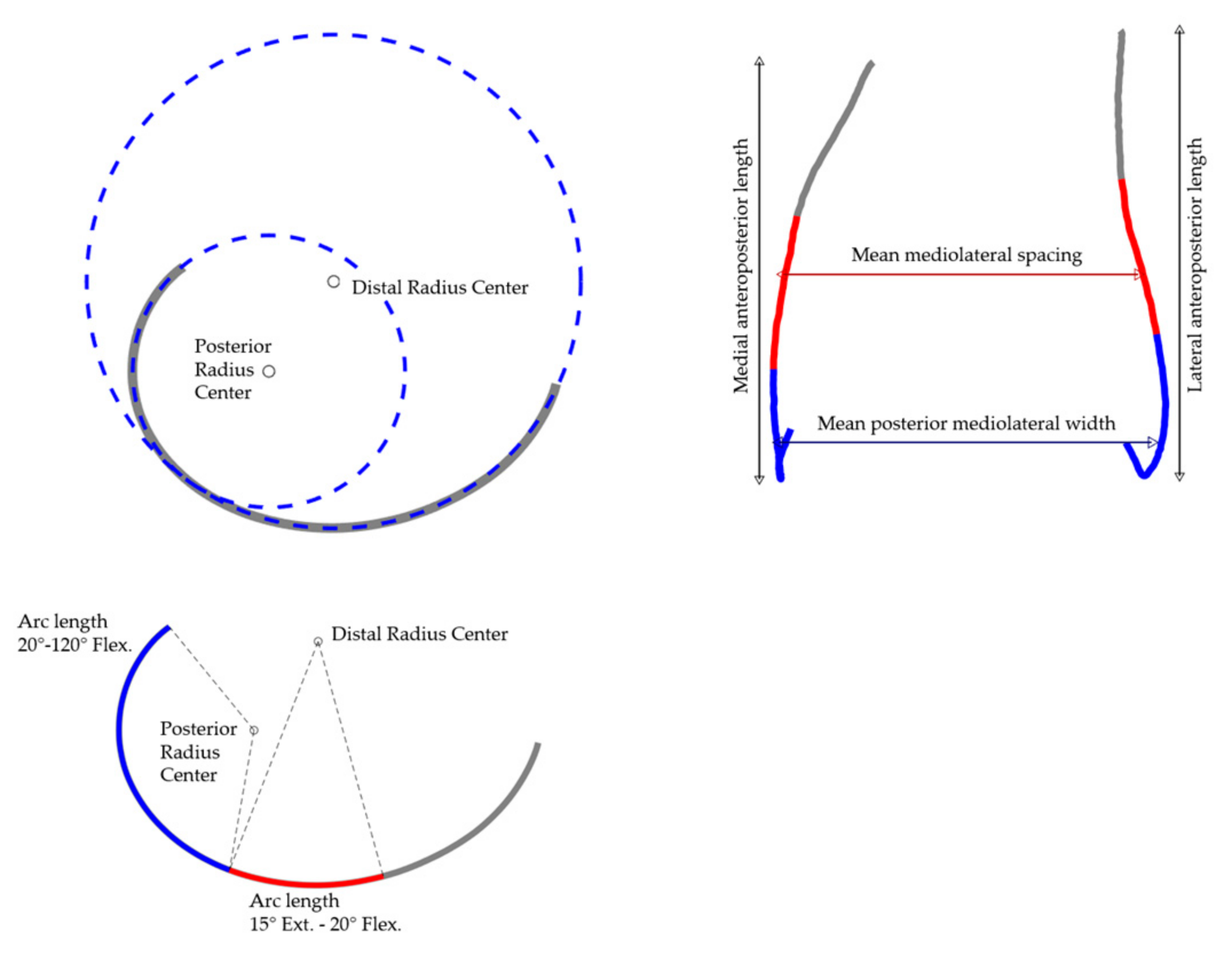
| Mean distal ML spacing | Overall | mm | Mean mediolateral distance of the distal points of the lateral/medial 3D J-Curve (15° of extension to 20° of flexion, reference: radius of the circle fitted to the distal portion of the condyles). Inspired by Walker [24]. |
| Mean posterior ML width | Overall | mm | Mean mediolateral distance of the posterior points of the lateral/medial 3D J-Curve (20°–120° of flexion, reference: radius of the circle fitted to the posterior portion of the condyles). Inspired by Mahfouz [25]. |
| AP length | Medial and lateral | mm | Anteroposterior length of the medial/lateral 3D J-Curve. |
| Distal radius | Medial and lateral | mm | Radius of the circle fitted to the distal portion of the medial/lateral 3D J-Curve. The calculation was performed according to Nuno and Ahmed [15] and is described in more detail in Asseln et al. [26]. |
| Posterior radius | Medial and lateral | mm | Radius of the circle fitted to the posterior portion of the medial/lateral 3D J-Curve. The calculation was performed according to Nuno and Ahmed [15] and is described in more detail in Asseln et al. [26]. |
| Functional arc length | Medial and lateral | mm | Arc length of the medial/lateral 3D J-Curve between 15° of extension until 120° of flexion (reference: center of the circle fitted to the distal/posterior portion of the condyles). |
| Arc length 15° Ext.–20° Flex. | Medial and lateral | mm | Arc length of the medial/lateral 3D J-Curve between 15° of extension until 20° of flexion (reference: center of the circle fitted to the distal portion of the condyles). |
| Arc length 20°–120° Flex. | Medial and lateral | mm | Arc length of the medial/lateral 3D J-Curve between 20° until 120° of flexion (reference: center of the circle fitted to the distal/ posterior portion of the condyles). |
| Mean abs. deviation | Medial and lateral | mm | Mean absolute deviation (mean condylar offset) regarding anteroposterior and proximodistal direction. |
| Max abs. deviation | Medial and lateral | mm | Maximum absolute deviation (maximum condylar offset) regarding anteroposterior and proximodistal direction. |
| Parameter (Normalized by ML/AP) | Mean ML Spacing | Mean Posterior ML Width | AP Length | Distal Radius | Posterior Radius | Funct. Arc Length | Arc Length 15°Ext.–20° Flex. | Arc Length 20°–120° Flex. | |
|---|---|---|---|---|---|---|---|---|---|
| Mean shape (combined) | 51.2 mm (0.95) | 53.7 mm | Lateral | 64.2 mm (0.99) | 48.8 mm (0.75) | 20.3 mm (0.31) | 67.4 mm (1.04) | 32.5 mm (0.50) | 34.9 mm (0.54) |
| Medial | 60.1 mm (0.93) | 35.1 mm (0.54) | 19.3 mm (0.30) | 67.5 mm (1.04) | 22.8 mm (0.35) | 44.7 mm (0.69) | |||
| Mean shape (Male) | 53.7 mm (0.96) | 56.1 mm | Lateral | 66.9 mm (0.99) | 50.5 mm (0.75) | 21.4 mm (0.32) | 69.7 mm (1.03) | 33.7 mm (0.50) | 35.9 mm (0.53) |
| Medial | 62.8 mm (0.93) | 36.9 mm (0.55) | 20.2 mm (0.30) | 70.1 mm (1.04) | 23.9 mm (0.36) | 46.2 mm (0.69) | |||
| Mean shape (Female) | 46.2 mm (0.94) | 49.1 mm | Lateral | 60.5 mm (0.99) | 46.9 mm (0.77) | 18.6 mm (0.31) | 64.0 mm (1.05) | 30.9 mm (0.51) | 33.2 mm (0.54) |
| Medial | 55.2 mm (0.91) | 31.5 mm (0.52) | 17.7 mm (0.29) | 62.9 mm (1.03) | 20.4 mm (0.33) | 42.5 mm (0.70) |
| Parameter | Mean ML Spacing | Mean Posterior ML Width | AP Length | Distal Radius | Posterior Radius | Funct. Arc Length | Arc Length 15°Ext.–20° Flex. | Arc Length 20°–120° Flex. | Mean Abs. Deviation | ||
|---|---|---|---|---|---|---|---|---|---|---|---|
| Mode | 1 | 11.79 mm (23.0%) | 10.96 mm (20.4%) | Lateral | 12.15 mm (18.9%) | 7.31 mm (15%) | 4.85 mm (23.9%) | 12.3 mm (18.3%) | 5.42 mm (16.7%) | 6.88 mm (19.7%) | 5.34 mm |
| Medial | 16.84 mm (28%) | 8.31 mm (23.7%) | 5.26 mm (27.2%) | 13.35 mm (19.8%) | 6.01 mm (26.4%) | 7.35 mm (16.4%) | 8.81 mm | ||||
| 2 | 3.71 mm (7.2%) | −0.3 mm (−0.6%) | Lateral | −7.11 mm (−11.1%) | 2.33 mm (4.8%) | 0.54 mm (2.7%) | 10.85 mm (16.1%) | 1.56 mm (4.8%) | 9.29 mm (26.6%) | 9.36 mm | |
| Medial | 3.4 mm (5.7%) | 1.99 mm (5.7%) | 0.87 mm (4.5%) | 6.84 mm (10.1%) | 1.72 mm (7.6%) | 5.12 mm (11.4%) | 4.56 mm | ||||
| 3 | 4.72 mm (9.2%) | 7.7 mm (14.3%) | Lateral | 6.59 mm (10.3%) | 9 mm (18.4%) | 3.44 mm (16.9%) | 16.2 mm (24%) | 7.76 mm (23.9%) | 8.44 mm (24.2%) | 4.37 mm | |
| Medial | 3.32 mm (5.5%) | 4.08 mm (11.6%) | 2.53 mm (13.1%) | 11.75 mm (17.4%) | 2.82 mm (12.4%) | 8.93 mm (20%) | 7.08 mm | ||||
| 4 | −4.72 mm (−9.2%) | −6.31 mm (−11.7%) | Lateral | 6.49 mm (10.1%) | 7.97 mm (16.3%) | 1.75 mm (8.6%) | 12.93 mm (19.2%) | 6.17 mm (19%) | 6.76 mm (19.4%) | 3.86 mm | |
| Medial | 2.63 mm (4.4%) | −0.24 mm (−0.7%) | 0.29 mm (1.5%) | 3.45 mm (5.1%) | −0.07 mm (−0.3%) | 3.52 mm (7.9%) | 2.09 mm | ||||
| 5 | −0.56 mm (−1.1%) | −0.72 mm (−1.3%) | Lateral | −0.49 mm (−0.8%) | −3.33 mm (−6.8%) | −0.17 mm (−0.8%) | −4.02 mm (−6%) | −1.61 mm (−4.9%) | −2.4 mm (−6.9%) | 2.97 mm | |
| Medial | 4.48 mm (7.4%) | 3.28 mm (9.3%) | 0.76 mm (3.9%) | 6.22 mm (9.2%) | 2.39 mm (10.5%) | 3.83 mm (8.6%) | 3.66 mm | ||||
Publisher’s Note: MDPI stays neutral with regard to jurisdictional claims in published maps and institutional affiliations. |
© 2021 by the authors. Licensee MDPI, Basel, Switzerland. This article is an open access article distributed under the terms and conditions of the Creative Commons Attribution (CC BY) license (https://creativecommons.org/licenses/by/4.0/).
Share and Cite
Grothues, S.A.G.A.; Radermacher, K. Variation of the Three-Dimensional Femoral J-Curve in the Native Knee. J. Pers. Med. 2021, 11, 592. https://doi.org/10.3390/jpm11070592
Grothues SAGA, Radermacher K. Variation of the Three-Dimensional Femoral J-Curve in the Native Knee. Journal of Personalized Medicine. 2021; 11(7):592. https://doi.org/10.3390/jpm11070592
Chicago/Turabian StyleGrothues, Sonja A. G. A., and Klaus Radermacher. 2021. "Variation of the Three-Dimensional Femoral J-Curve in the Native Knee" Journal of Personalized Medicine 11, no. 7: 592. https://doi.org/10.3390/jpm11070592