Article

Histopathological Image Diagnosis for Breast Cancer Diagnosis Based on Deep Mutual Learning

by
Amandeep Kaur
1,
Chetna Kaushal
1,
Jasjeet Kaur Sandhu
1,
Robertas Damaševičius
2,* and
Neetika Thakur
3
1
Chitkara University Institute of Engineering and Technology, Chitkara University, Rajpura 140401, India
2
Department of Applied Informatics, Vytautas Magnus University, 53361 Akademija, Lithuania
3
Junior Laboratory Technician, Postgraduate Institute of Medical Education and Research, Chandigarh 160012, India
*
Author to whom correspondence should be addressed.
Diagnostics 2024, 14(1), 95; https://doi.org/10.3390/diagnostics14010095
Submission received: 12 November 2023 / Revised: 26 December 2023 / Accepted: 28 December 2023 / Published: 31 December 2023

Abstract

:
Every year, millions of women across the globe are diagnosed with breast cancer (BC), an illness that is both common and potentially fatal. To provide effective therapy and enhance patient outcomes, it is essential to make an accurate diagnosis as soon as possible. In recent years, deep-learning (DL) approaches have shown great effectiveness in a variety of medical imaging applications, including the processing of histopathological images. Using DL techniques, the objective of this study is to recover the detection of BC by merging qualitative and quantitative data. Using deep mutual learning (DML), the emphasis of this research was on BC. In addition, a wide variety of breast cancer imaging modalities were investigated to assess the distinction between aggressive and benign BC. Based on this, deep convolutional neural networks (DCNNs) have been established to assess histopathological images of BC. In terms of the Break His-200×, BACH, and PUIH datasets, the results of the trials indicate that the level of accuracy achieved by the DML model is 98.97%, 96.78, and 96.34, respectively. This indicates that the DML model outperforms and has the greatest value among the other methodologies. To be more specific, it improves the results of localization without compromising the performance of the classification, which is an indication of its increased utility. We intend to proceed with the development of the diagnostic model to make it more applicable to clinical settings.

1. Introduction

Breast cancer (BC) is the most common kind of cancer in women, accounting for around 30% of all new cancer diagnoses; it is also the second most fatal malignancy after lung and bronchial cancers [1]. According to the most recent data from the International Agency for Research on Cancer, which is part of the World Health Organization, breast cancer has exceeded lung cancer as the most frequent cancer, with 2.26 million new cases in 2020, overtaking lung cancer. It presents a major threat to the lives and health of women. Early diagnosis is crucial in the fight against cancer, and this can only be achieved with a reliable detection system. Two techniques that have been developed to aid in the diagnosis of breast cancer are medical image processing and digital pathology, respectively [2,3,4]. BC has two particularly alarming features among the many forms of cancer: being the most frequent disease in women across the globe and having a much higher fatality rate than additional kinds of cancer, because the histopathological examination is the most often utilized approach for the diagnosis of breast cancer. In many cases, pathologists still use the visual evaluation of histological samples beneath the microscope to make a diagnosis. Automated histopathological image classification is a study area that might speed up and reduce the risk of mistakes in BC diagnosis [5]. Histopathology uses a biopsy to obtain images of the diseased tissue [6,7]. Early identification is significant for illness treatment and a safer prognosis [8]. Noninvasive BC screening procedures include clinical breast assessment and tomography tests, such as magnetic resonance, ultrasound, and mammography. However, the requirement for verifying the identification of BC is the pathological study of a slice of the suspicious region by a diagnostician. Glass slides tarnished with hematoxylin and eosin are used to examine the microscopic details of the questionable tissue [9]. There are various analytical modes used for BC detection. Some of the general modes are mammography, magnetic resonance imaging (MRI), positron emission tomography (PET), breast ultrasound, surgery, or fine-needle aspiration to target the nerve of the alleged area (histopathological images), etc., as shown in Figure 1 [10,11].
Different methods, such as rule-based and machine-learning approaches, are used to evaluate breast cancer digital pathology images [12]. Recently, it has been shown that deep-learning-based approaches, which automate the whole processing, outperform classical machine-learning techniques in numerous image-assessment tasks [13]. Successful applications of convolutional neural networks (CNNs) in medical imaging have allowed for the early diagnosis of diabetic retinopathy, the prediction of bone disease and age, and other problems. Earlier deep-learning-based functions in histological microscopic image processing have demonstrated their capacity to be effective in the detection of breast cancer. Machine learning has played an increasingly important role in breast cancer detection over the last several decades. Several probabilistic, statistical, and optimization strategies could be used in the machine-learning approach to derive a classification model from a dataset [14].
Breast carcinoma is a commonly classified histopathology established on the selection of morphological aspects of the cancers, with 20 main cancer categories and 18 lesser subtypes. Invasive ductal carcinoma (IDC) and invasive lobular carcinoma (ILC) are the two primary histological groups of breast cancer, with approximately 70–80% of all cases falling into one of these categories [15,16]. Deep-learning (DL) methods are capable of autonomously extracting features, retrieving information from data, and learning sophisticated abstract interpretations of the data. DL techniques are powerful. They can resolve typical feature-extraction issues and have found use in a selection of sectors, including computer vision and biomedicine.
Centered on deep convolutional neural networks, a new BC histopathological image category blind inpainting convolutional neural network (BiCNN) model has been developed. It was developed to cope with the two-class categorization of BC on the diagnostic image. The BiCNN model uses previous knowledge of the BC class and subclass labels to constrain the distance between the characteristics of distinct BC pathology images [17]. A data-augmented technique is provided to suit the acceptance of whole-slide image identification [18]. The transfer-fine-tuning training approach is employed as an appropriate training approach [19] to increase the accuracy of BC histological image categorization. Figure 2 and Figure 3 demonstrate some of the finer characteristics of the pathological images of BC. Samples (a) through (e) in Figure 2 are all ductal carcinomas (DCs). The phyllodes tumor is sample (f). The colors and forms of the cells in samples (a)–(e) all belong to DCs, even though they are all DC samples. Samples (e) and (f) have a striking resemblance in terms of color and cell shape; however, they are classified as distinct classes. Figure 3 depicts abnormal images at various magnification levels. There is a substantial variance in the visual features across the various magnifications, even though they are all from the same subject [20].

2. Literature Review

The National Institute of Oncology in Rabat, Morocco, received 116 surgical breast specimens with invasive cancer of an unknown nature, resulting in 328 digital slides. These photos were properly classified into one of three types: normal tissue–benign lesions, in situ cancer, or aggressive carcinoma. It was shown that, despite the small size of the dataset, the classification model developed in this research was able to accurately predict the likelihood of a BC diagnosis [21]. To compare the performance of chronic myelogenous leukemia (CML)- and DL-based techniques, the author also provided a visual analysis of the histological results to categorize breast cancer. CML-based approaches utilize three feature extractors to extract hand-crafted features and combine them to build an image representation for five traditional classifiers. The DL-based techniques utilized the well-known VGG-19 DL design, which was fine-tuned using histopathological images. The data showed that the DL methods outperformed the CML methods, with an accuracy range of 94.05 to 98.13% for the binary classification and 76.77 to 88.95% for the eighth-class classification [22]. The DCNN-based heterogeneous ensemble method for mitotic nuclei identification was used for breast histopathology images using the DHE-Mit-Classifier. Histopathological biopsy samples were examined for the presence of mitotic patches, and the DHE-Mit-Classifier was used to sort them into mitotic and nonmitotic nuclei. A heterogeneous ensemble was constructed using five independent DCNNs. the mitotic nuclei’s structural, textural, and morphological characteristics remain captured by these DCNNs, which included a variety of architectural styles. The recommended ensemble had an F-score of 0.77, a recall of 0.71, a precision of 0.83, and an area under the curve (AUC) accuracy–recall of 0.83, which surpassed the test set of 0.80. The F-score and accuracy indicated that this ensemble might be utilized to build a pathologist’s helper [23]. The BC patients benefited from the enhanced and multiclass whole-slide imaging (WSI) segmentation uses of the CNN. These components organize information collected from CNNs into pathologists’ predictions. Pathologists need instruments that can speed up the time to perform histological analyses, provide a second opinion, or even point out areas of concern during routine screening. This yielded a sensitivity of 90.77%, a precision of 91.27%, an F1 score of 84.17%, and a specificity of 94.03%. The area subdivision module acquired a sensitivity of 71.83%, an IOU of 88.23%, an intersection over union (IOU) of 93.43%, a precision of 96.10%, an F1 score of 82.94%, a specificity of 96.19%, and an AUC of 0.88 for the improved WSI segmentation [24]. A hybrid model based on DCNNs and pulse-coupled neural networks (PCNNs) was developed. Transfer learning (TL) was used in this study due to the necessity for huge datasets to train and tune the CNNs, which were not accessible for medical images. TL can be an efficient method when dealing with tiny datasets. The document’s application was assessed using three public standard datasets, DDMS, INbreast, and BCDR, for the instruction and analysis, and MIAS for testing alone. The findings demonstrated the benefit of combining the PCNN with the CNN over other approaches for the same public datasets. The hybrid model accurately predicted DDMS (98.72%), BCDR (96.94%), and breast cancer (97.5%). The proposed hybrid model was tested on a previously unreported MIAS dataset and showed an accuracy of 98.7%. In the Results section, further assessment measures can be found [25]. There are a variety of digital pathology image-evaluation techniques for breast cancer, including rule-based and machine-learning approaches [26]. Lately, DL-based processes have been proven to outpace traditional machine-learning techniques in several image-evaluation tasks, computerizing the whole-processing process [27]. Convolution neural networks (CNNs) have been utilized effectively in the medical imaging field to detect diabetic retinopathy, forecast bone disease and age, and other issues. Earlier DL-based functions in histological microscopic image processing have shown their ability to be useful in the diagnosis of breast cancer. The detection of BC has become more dependent on machine learning over the last several decades. The machine-learning method includes a variety of probabilistic, statistical, and optimization techniques for deriving a classification model from a dataset [28].

3. Research Methodology

This section explains the suggested methodology of the research work. In this methodology, the procedure is categorized into four categories: visual synonyms, image segmentation, similarity, and model training. DML and label propagation are two techniques that are employed in this approach for explainable BC histopathological image diagnosis. This process includes a draught for visual synonyms with a fuzzy set of criteria, as well as the generation of real synonyms and the expansion of the keyword list. An image dataset is used, which was generated, that contains the following elements: image preprocessing, revision and normalization of the input image, image segmentation, and the segment difference score using label propagation. After completing the image segmentation and visual synonym processes, it generates the similarity between them; finally, it performs model training with the aid of the DML approach.
The techniques used in the proposed methodology are discussed below.

3.1. Training Based on DML

The actual process used to autonomously train the proposed model is described as the subsequent multiclass cross-entropy loss:
L C = ( y C · l o g C 1 y C · l o g 1 C )
where C is the possibility that a bag is expected as a positive classification and y C 0, 1 suggests that a histopathological image is expected to be malignant or benign.
The analysis model is accomplished separately in typical circumstances, which does not allow for the diagnostic model’s full potential to be tapped. The goal is to train two models in a cohort using the DML schema as shown in Figure 4. [29]. As illustrated in Figure 5, θ 1 and θ 2 are two indistinguishable entities (networks) of the model. Two same bags are input into the DML structure at a similar moment; P 1 , P 2 R 2 × 1 are the outputs of every individual network.
Let P 1 1 and P 1 1 signify the possibility that θ 1 forecasts that a bag goes to the positive and negative classes, separately. The KL distance from P 1 to P 2 is calculated as
D K L = P 2 0 l o g P 2 0 P 1 0 + P 2 1 l o g P 2 1 P 1 1
The total loss functions L θ 1 and L θ 2 for the θ1 and θ2 networks are thus achieved, correspondingly, as follows:
L θ 1 = L C 1 + D K L ( P 2 ǁ P 1 )
L θ 2 = L C 2 + D K L ( P 1 ǁ P 2 )
The loss LC and the KL mimicry loss teach every network to forecast the correct description of the input bag and to match the possible value of its peer network. They can convert the initial DML schema from supervised to inadequately supervised learning in this way. Furthermore, the DML architecture allows for bidirectional information transfer via collective training in a cohort, as well as the ability to tap into the model’s capacity for the accurate categorization of the histopathology images [30].
BreakHis, BACH, and PUIH are all publicly accessible BC histopathology image datasets used to validate the proposed DML model. There are 7909 histopathological images in the BreakHis dataset, each with three channels and four magnifications. PUIH has 4020 three-channel images, while BACH contains 400. The magnification of the images in these two datasets is not specified. BACH and PUIH include 2048 × 1536 pixel images, while BreakHis has images that are 700 × 460 pixels in size. An in-depth look at the three datasets is provided in Table 1. Figure 5 shows a selection of these photos.

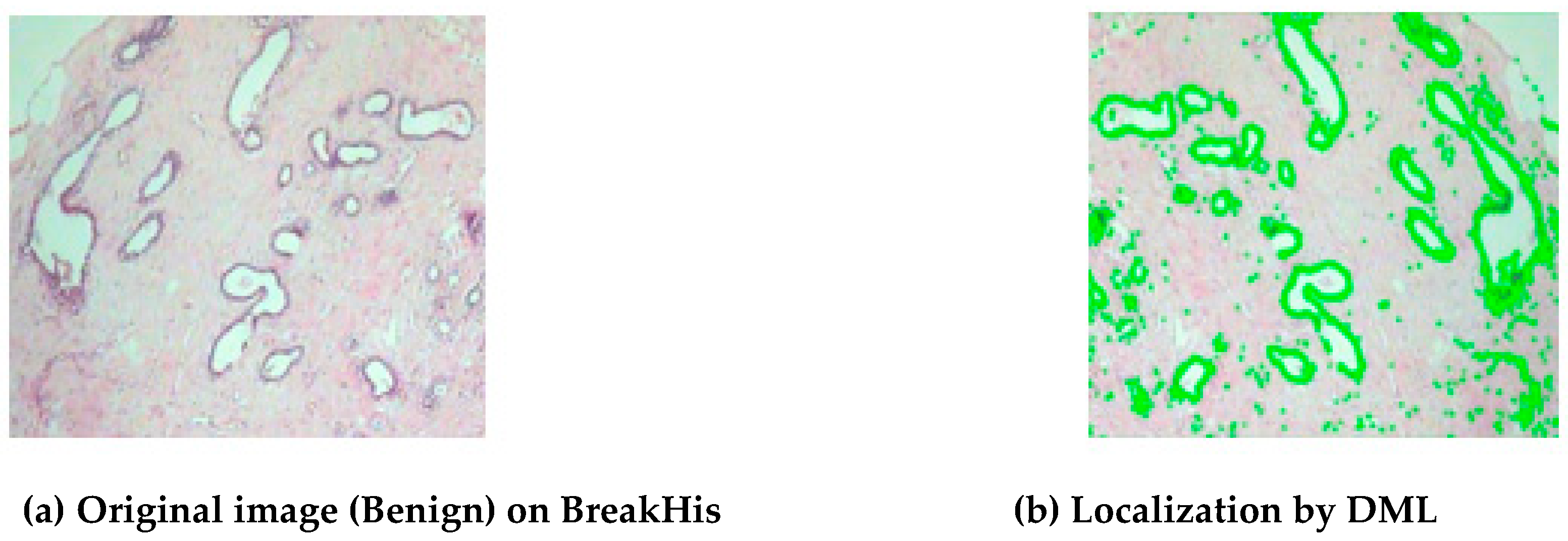
3.2. Label Propagation for Image Segmentation

Label propagation is a semisupervised machine-learning method that adds labels to data points that were previously unlabeled. Image segmentation is an essential component of various image-processing systems. Few computerized image-analysis approaches can be used autonomously with good results in most circumstances [31].
The term interactive segmentation comes from the fact that semiautomated segmentation algorithms enable users to engage in the segmentation process and provide some direction for the description of the required material to be retrieved [32]. An interactive segmentation algorithm that works in practice must have four qualities: quick calculation, quick editing, the capacity to create arbitrary segmentation given enough interactions, and understandable segmentation. Active-contour- or level-set-based approaches, as well as graph-cut-based methods, have been presented in the recent several decades for image segmentation.
Although these algorithms have been successful in many circumstances, there are still a few issues with their use. It is difficult to execute the level-set-based or active-contour solutions; subsequently, the user must input the many free factors. The graph-cut-based systems only replace the tiniest cut that separates the seeds (i.e., the labeled pixels), and they typically provide the tiny reductions that simply divide the seeds from the remaining pixels when the number of seeds is extremely small.

3.3. Proposed Methodology

This section provides the in-depth detail of the proposed methodology. The proposed methodology block diagram is shown in Figure 6 below:
Step 1: Input Image Dataset
This is the collection of images with which the analysis will be performed.
Step 2: Image Preprocessing
The initial step involves revising and normalizing the input images. This could include tasks like resizing, cropping, or adjusting the color levels to prepare the images for further analysis.
Step 3: Image Segmentation
Image segmentation involves dividing an image into different segments to identify and analyze different regions. This can be useful for tasks like object recognition or scene understanding.
Step 4: Segment Difference Score using Label Propagation
This step suggests assigning scores to the segmented regions, possibly using a label-propagation technique. Label propagation is a semisupervised learning method that can be used to propagate labels from a small set of labeled data to unlabeled data.
Step 5: Draft Keyword for Better Interpretability with a Fuzzy Set of Rules
This step involves generating keywords that help in interpreting the results. Fuzzy set theory might be employed here to handle uncertainty in the data.
Step 6: Generate Actual Synonyms and Expand the Keyword List
This step implies creating synonyms for the drafted keywords and expanding the keyword list to capture a broader range of concepts related to the analysis.
Step 7: Generate Similarity for Visual Synonyms and Image Segmentation
This involves assessing the similarity between visual synonyms (possibly the segmented regions) and the results of the image segmentation.
Step 8: Model Training Using the Same Deep Mutual Learning
Deep mutual learning usually refers to training models collaboratively. In this context, it suggests training a model using the information gained from the image segmentation and the fuzzy set of rules.
Step 9: Output
Based on the training, the output of the model is generated in this step, which is associated with the state-of-the-art technique based on various parameters (AUC, precision, recall).
These steps are summarized as Algorithm 1.
Algorithm 1 Deep Mutual Learning for Breast Cancer Histopathology Image Diagnosis
Require: Image datasets (BreakHis, BACH, PUIH)
Ensure: Trained model for breast cancer histopathology image diagnosis
1: Initialize two identical neural network models θ1; and θ2
2: for each batch of input images do
3:   Preprocess images (revision, normalization)
4:   Perform image segmentation
5:   Calculate segment difference score using label propagation
6:   Compute multi-class cross-entropy loss LC for each model
7:   LC = −(yC · logC) + (1 − yC) · log(1 − ΦC))
8:   Calculate KL divergence DkL, between the two models
9:   DKL = P20 · log(P20/P10) + P21 · log(P21/P11)
10:    Update total loss functions for each model
11:    Lθ1 = LC1 + DKL(P2 || P1)
12:    Lθ2 = LC2 + DKL(P1 || P2)
13:    Train both models using the computed losses
14: end for
15: Repeat steps 2–11 until convergence
16: Evaluate the trained model on test datasets

4. Results

In this part of the study, the implementation that was carried out utilizing the technique that was suggested is presented. MATLAB 2020 (Mathworks India Private Limited, Bangalore, India) was used as a functional tool.
The BreakHis, BACH, and PUIH BC histopathology image datasets were used to test the suggested DML. A receiver operating characteristic (ROC) curve was used to assess the suggested model’s accuracy objectively and fully, among other evaluation criteria, i.e., the AUC.
Figure 7, Figure 8 and Figure 9 demonstrate the parallel ROC curve and AUC value on every dataset. The results that are shown in Figure 8 illustrate the ROC curves and the AUC values for the BreakHis-200× dataset. The MA-MIDN-Ind model and the MA-MIDN-DML model lag behind the DML model. Considering all of them, it seems that DML performs a role that is energetic. In addition to enhancing the accuracy of the final organization, it could additionally validate the potential of the model to simplify complex situations by using the BreakHis dataset.
The ROC curve and the area under the curve (AUC) value for the BACH dataset are shown in Figure 8, which describes the outcome. It is of the greatest significance that the DML on the BACH dataset be accurate when it comes to the MA-MIDN model (both the MA-MIDN-DML model and the MA-MIDN-Ind model simultaneously). These data can be made use of in order to demonstrate and enhance the generalization capabilities of the model.
Figure 9 displays the ROC curve and AUC value for the PUH dataset. The AUC of the DML using the PUIH dataset is critical in the MA-MIDN model’s performance (the MA-MIDN-DML model and MA-MIDN-Ind model). It has the potential to demonstrate the correctness of the model while also increasing the generalization capacity of the model.
Table 2 illustrates the comparison of the current methodologies with the proposed methodology. Table 2 and Figure 10 show that the proposed DML model beats the MA-MIDN-DML model and the MA-MIDN-Ind model by a large margin on the BreakHis, BACH, and PUIH datasets.
Figure 11 displays the findings for all datasets in terms of localization. The objective and complete evaluation of the obtained localization findings is based on both benign and malignant images with varying morphologies. Figure 11a shows the original image on BreakHis dataset and Figure 11b shows the localization outcome by DML on BreaKHis dataset. Figure 12 shows different attention processes’ localization outcomes on the BACH dataset. Figure 12a shows the original image of BACH dataset and Figure 12b shows the Localization outcome by DML on BACH dataset.
A variety of current methodologies are examined on each dataset to see how well the suggested model performs. On the BreakHis dataset, we first evaluated our model compared to the following baseline styles: Res Hist-Aug, FCN + Bi LSTM, MI-SVM, Deep MIL, and the MA-MIDN model. Table 3 shows the results of the accuracy comparisons.
Table 4 shows the differences of UC, precision, recall and F1 on Breakhis dataset. As compared to BreakHis, BACH, and PUIH (the most recent dataset to be published in 2020), the images have a greater resolution. So, the DML model has a major hurdle in classifying the two datasets. The Patch + Vote, B + FA + GuSA, Hybrid-DNN, and MA-MIDN are the baseline models against which we compared our model on the BACH and PUIH datasets. The comparisons of the performances are shown in Table 5.
The Grad-CAM approach was used in conjunction with the ResNet50 model, which was trained on the BACH dataset. Figure 13a,b shows the breast glands from the original image of BACH dataset. Figure 13a’,b’ shows the GRAD-CAM patch based localization findings with ResNet50 model.
The DML was compared to the other popular pooling approaches. It directly performs max and means pooling on instance-level features to achieve the test results. Figure 14 displays the results of the analysis.
The appropriate experimental outcomes are shown in Table 6, employing the MI-Net and running tests on three datasets; “No Attention” yields its findings [36].
The DML model’s localization results consume most of the testing time, as shown in Table 7 and Table 8. This dataset has a lower image size than the previous two; therefore, the DML model runs quicker on it. For the BACH and PUIH datasets, the average classification time of the DML model was 0.09 s, while the average classification time for simultaneous localization was 1.55 s. These numbers are satisfactory to a certain degree, but they could be improved upon further.
A unique multiview attention-guided multiple-instance detection network (MA-MIDN) is presented to address this issue. Multiple-instance learning (MIL) can be used to solve the classic image-categorization issue. It first separates each histopathological image into instances and then builds a matching bag to obtain the maximum use of the high-resolution data provided by the MIL. A novel multiple-view attention (MVA) technique is presented to train the awareness of the occurrences in the image to identify the wound locations in this image. An MVA-guided MIL sharing technique is intended to aggregate instance-level characteristics to acquire the bag-level characteristics for the last organization. The suggested MA-MIDN standard operates image classification as well as lesion localization at the same time. The MA-MIDN model is specifically trained using DML. DML is now a poorly supervised learning issue. Three community BC histopathology image datasets were used to test the categorization and localizations findings. The investigational findings indicate that the MA-MIDN model outperforms the most recent criteria in conditions of diagnostic precision, AUC, recall, precision, and the F1-score. Specifically, it delivers improved localization outcomes without sacrificing categorization performance, indicating its greater usefulness [29].

5. Conclusions and Future Scope

Advances in DL techniques have proven a substantial improvement in the diagnosis of BC histopathology images. Even with the use of high-resolution histopathology images, training and interpretable diagnostic models remain a difficult endeavor. The DML approach is being considered to ease this difficulty. Compared to the prior approach on three datasets (Break His, BACH, and PUIH), the suggested technique outperforms the previous technique. The accuracy of the suggested approach shows that the DML model, in the terms of Break His-200×, BACH, and PUIH datasets (98.97%, 96.78%, and 96.34%), outperform the highest value of the current techniques. The proposed approach provides for quicker data transfer, since it reduces the propagation delay. As a result, the suggested approach outperformed the current technique when compared to it.
The proposed model could be further expanded in the future to provide better functionality in terms of protecting the confidentiality of users and providing the quality of data collected by medical institutions. Its goal is to enhance the implementation of the diagnostic model to make it useful in clinical practice.

Author Contributions

Conceptualization, A.K.; methodology, A.K.; software, A.K., C.K., J.K.S. and N.T.; validation, A.K., C.K., J.K.S., R.D. and N.T.; formal analysis, A.K., C.K., J.K.S., R.D. and N.T.; investigation, A.K., C.K., J.K.S., R.D. and N.T.; resources, A.K.; writing—original draft preparation, A.K., C.K. and J.K.S.; writing—review and editing, R.D.; visualization, A.K., C.K. and J.K.S.; supervision, A.K. All authors have read and agreed to the published version of the manuscript.

Funding

This research received no external funding.

Institutional Review Board Statement

Not applicable.

Informed Consent Statement

Not applicable.

Data Availability Statement

The BreakHis dataset is available at: https://web.inf.ufpr.br/vri/databases/breast-cancer-histopathological-database-breakhis/ (accessed on 5 July 2022). The BACH dataset is available at: https://zenodo.org/records/3632035 (accessed on 5 July 2022).

Conflicts of Interest

The authors declare no conflicts of interest.

References

  1. Siegel, R.L.; Miller, K.D.; Fedewa, S.A.; Ahnen, D.J.; Meester, R.G.; Barzi, A.; Jemal, A. Colorectal cancer statistics, 2017. CA Cancer J. Clin. 2017, 67, 177–193. [Google Scholar] [CrossRef] [PubMed]
  2. Spanhol, F.A.; Oliveira, L.S.; Cavalin, P.R.; Petitjean, C.; Heutte, L. Deep features for breast cancer histopathological image classification. In Proceedings of the 2017 IEEE International Conference on Systems, Man and Cybernetics (SMC), Banff, AB, Canada, 5–8 October 2017; pp. 1868–1873. [Google Scholar]
  3. Desai, M.; Shah, M. An anatomization on breast cancer detection and diagnosis employing multi-layer perceptron neural network (MLP) and Convolutional neural network (CNN). Clin. eHealth 2021, 4, 1–11. [Google Scholar] [CrossRef]
  4. Alanazi, S.A.; Kamruzzaman, M.M.; Sarker, N.I.; Alruwaili, M.; Alhwaiti, Y.; Alshammari, N.; Siddiqi, M.H. Boosting Breast Cancer Detection Using Convolutional Neural Network. J. Health Eng. 2021, 2021, 5528622. [Google Scholar] [CrossRef] [PubMed]
  5. Lakhani, S.R.; Ellis, I.O.; Schnitt, S.; Tan, P.; van de Vijver, M. WHO Classification of Tumors of the Breast, 4th ed.; WHO Press: Geneva, Switzerland, 2012; Volume 4.
  6. Das, A.; Devarampati, V.K.; Nair, M.S. NAS-SGAN: A Semi-Supervised Generative Adversarial Network Model for Atypia Scoring of Breast Cancer Histopathological Images. IEEE J. Biomed. Health Inform. 2021, 26, 2276–2287. [Google Scholar] [CrossRef] [PubMed]
  7. Liu, Y.; Li, A.; Liu, J.; Meng, G.; Wang, M. TSDLPP: A Novel Two-Stage Deep Learning Framework for Prognosis Prediction Based on Whole Slide Histopathological Images. IEEE/ACM Trans. Comput. Biol. Bioinform. 2021, 19, 2523–2532. [Google Scholar] [CrossRef] [PubMed]
  8. World Health Organization. Cancer. 2019. Available online: https://www.who.int/health-topics/cancer (accessed on 15 June 2022).
  9. Bejnordi, B.E.; Zuidhof, G.; Balkenhol, M.; Hermsen, M.; Bult, P.; van Ginneken, B.; Karssemeijer, N.; Litjens, G.; van der Laak, J. Context-aware stacked convolutional neural networks for classification of breast carcinomas in whole-slide histopathology images. J. Med. Imaging 2017, 4, 044504. [Google Scholar] [CrossRef] [PubMed]
  10. Houssein, E.H.; Emam, M.M.; Ali, A.A.; Suganthan, P.N. Deep and machine learning techniques for medical imaging-based breast cancer: A comprehensive review. Expert Syst. Appl. 2021, 167, 114161. [Google Scholar] [CrossRef]
  11. Houssein, E.H.; Emam, M.M.; Ali, A.A. An efficient multilevel thresholding segmentation method for thermography breast cancer imaging based on improved chimp optimization algorithm. Expert Syst. Appl. 2021, 185, 115651. [Google Scholar] [CrossRef]
  12. Zebari, D.A.; Ibrahim, D.A.; Zeebaree, D.Q.; Haron, H.; Salih, M.S.; Damaševičius, R.; Mohammed, M.A. Systematic Review of Computing Approaches for Breast Cancer Detection Based Computer Aided Diagnosis Using Mammogram Images. Appl. Artif. Intell. 2021, 35, 2157–2203. [Google Scholar] [CrossRef]
  13. Gupta, I.; Gupta, S.; Singh, S. Different CNN-based Architectures for Detection of Invasive Ductal Carcinoma in Breast Using Histopathology Images. Int. J. Image Graph. 2021, 21, 2140003. [Google Scholar] [CrossRef]
  14. Ogundokun, R.O.; Misra, S.; Douglas, M.; Damaševičius, R.; Maskeliūnas, R. Medical Internet-of-Things Based Breast Cancer Diagnosis Using Hyperparameter-Optimized Neural Networks. Futur. Internet 2022, 14, 153. [Google Scholar] [CrossRef]
  15. Motlagh, M.H.; Jannesari, M.; Aboulkheyr, H.; Khosravi, P.; Elemento, O.; Totonchi, M.; Hajirasouliha, I. Breast cancer histopathological image classification: A deep learning approach. bioRxiv 2018. [Google Scholar] [CrossRef]
  16. Sharma, S.; Mehra, R. Conventional Machine Learning and Deep Learning Approach for Multi-Classification of Breast Cancer Histopathology Images—A Comparative Insight. J. Digit. Imaging 2020, 33, 632–654. [Google Scholar] [CrossRef] [PubMed]
  17. Wei, B.; Han, Z.; He, X.; Yin, Y. Deep learning model-based breast cancer histopathological image classification. In Proceedings of the 2017 IEEE 2nd International Conference on Cloud Computing and Big Data Analysis (ICCCBDA), Chengdu, China, 28–30 April 2017; pp. 348–353. [Google Scholar]
  18. Oyewola, D.O.; Dada, E.G.; Misra, S.; Damaševičius, R. A Novel Data Augmentation Convolutional Neural Network for Detecting Malaria Parasite in Blood Smear Images. Appl. Artif. Intell. 2022, 36, 2033473. [Google Scholar] [CrossRef]
  19. Diwakaran, M.; Surendran, D. Breast Cancer Prognosis Based on Transfer Learning Techniques in Deep Neural Networks. Inf. Technol. Control. 2023, 52, 381–396. [Google Scholar] [CrossRef]
  20. Li, L.; Pan, X.; Yang, H.; Liu, Z.; He, Y.; Li, Z.; Fan, Y.; Cao, Z.; Zhang, L. Multi-task deep learning for fine-grained classification and grading in breast cancer histopathological images. Multimed. Tools Appl. 2020, 79, 14509–14528. [Google Scholar] [CrossRef]
  21. El Agouri, H.; Azizi, M.; El Attar, H.; El Khannoussi, M.; Ibrahimi, A.; Kabbaj, R.; Kadiri, H.; BekarSabein, S.; EchCharif, S.; El Khannoussi, B. Assessment of deep learning algorithms to predict histopathological diagnosis of breast cancer: First Moroccan prospective study on a private dataset. BMC Res. Notes 2022, 15, 66. [Google Scholar] [CrossRef]
  22. Said, B.; Liu, X.; Wan, Y.; Zheng, Z.; Ferkous, C.; Ma, X.; Li, Z.; Bardou, D. Conventional machine learning versus deep learning for magnification dependent histopathological breast cancer image classification: A comparative study with a visual explanation. Diagnostics 2021, 11, 528. [Google Scholar]
  23. Sohail, A.; Khan, A.; Nisar, H.; Tabassum, S.; Zameer, A. Mitotic nuclei analysis in breast cancer histopathology images using deep ensemble classifier. Med. Image Anal. 2021, 72, 102121. [Google Scholar] [CrossRef]
  24. Zeiser, F.A.; da Costa, C.A.; Ramos, G.d.O.; Bohn, H.C.; Santos, I.; Roehe, A.V. DeepBatch: A hybrid deep learning model for interpretable diagnosis of breast cancer in whole-slide images. Expert Syst. Appl. 2021, 185, 115586. [Google Scholar] [CrossRef]
  25. Altaf, M.M. A hybrid deep learning model for breast cancer diagnosis based on transfer learning and pulse-coupled neural networks. Math. Biosci. Eng. 2021, 18, 5029–5046. [Google Scholar] [CrossRef] [PubMed]
  26. Robertson, S.; Azizpour, H.; Smith, K.; Hartman, J. Digital image analysis in breast pathology—From image processing techniques to artificial intelligence. Transl. Res. 2017, 1931–5244. [Google Scholar] [CrossRef] [PubMed]
  27. Ching, T.; Himmelstein, D.S.; Beaulieu-Jones, B.K.; Kalinin, A.A.; Do, B.T.; Way, G.P.; Ferrero, E.; Agapow, P.-M.; Xie, W.; Rosen, G.L.; et al. Opportunities and Obstacles for Deep Learning in Biology and Medicine. bioRxiv 2017. [Google Scholar] [CrossRef] [PubMed]
  28. Singh, S.; Kumar, R. Histopathological image analysis for breast cancer detection using cubic SVM. In Proceedings of the 2020 7th International Conference on Signal Processing and Integrated Networks (SPIN), Noida, India, 27–28 February 2020; pp. 498–503. [Google Scholar]
  29. Li, G.; Li, C.; Wu, G.; Ji, D.; Zhang, H. Multi-View Attention-Guided Multiple Instance Detection Network for Interpretable Breast Cancer Histopathological Image Diagnosis. IEEE Access 2021, 9, 79671–79684. [Google Scholar] [CrossRef]
  30. Spanhol, F.A.; Oliveira, L.S.; Petitjean, C.; Heutte, L. A Dataset for Breast Cancer Histopathological Image Classification. IEEE Trans. Biomed. Eng. 2016, 63, 1455–1462. [Google Scholar] [CrossRef] [PubMed]
  31. Breve, F. Interactive image segmentation using label propagation through complex networks. Expert Syst. Appl. 2019, 123, 18–33. [Google Scholar] [CrossRef]
  32. Kadry, S.; Rajinikanth, V.; Taniar, D.; Damaševičius, R.; Valencia, X.P.B. Automated segmentation of leukocyte from hematological images—a study using various CNN schemes. J. Supercomput. 2022, 78, 6974–6994. [Google Scholar] [CrossRef]
  33. Wan, T.; Cao, J.; Chen, J.; Qin, Z. Automated grading of breast cancer histopathology using cascaded ensemble with combination of multi-level image features. Neurocomputing 2017, 229, 34–44. [Google Scholar] [CrossRef]
  34. Gour, M.; Jain, S.; Kumar, T.S. Residual learning based CNN for breast cancer histopathological image classification. Int. J. Imaging Syst. Technol. 2020, 30, 621–635. [Google Scholar] [CrossRef]
  35. Budak, Ü.; Cömert, Z.; Rashid, Z.N.; Şengür, A.; Çıbuk, M. Computer-aided diagnosis system combining FCN and bi-LSTM model for efficient breast cancer detection from histopathological images. Appl. Soft Comput. 2019, 85, 105765. [Google Scholar] [CrossRef]
  36. Sudharshan, P.J.; Petitjean, C.; Spanhol, F.; Oliveira, L.E.; Heutte, L.; Honeine, P. Multiple instances learning for histopathological breast cancer image classification. Expert Syst. Appl. 2019, 117, 103–111. [Google Scholar] [CrossRef]
  37. Rony, J.; Belharbi, S.; Dolz, J.; Ayed, I.B.; McCaffrey, L.; Granger, E. Deep weakly-supervised learning methods for classification and localization in histology images: A survey. arXiv 2019, arXiv:1909.03354. [Google Scholar] [CrossRef]
  38. Ahmad, H.M.; Ghaffar, S.; Khurshid, K. Classification of breast cancer histology images using transfer learning. In Proceedings of the 16th International Bhurban Conference on Applied Sciences and Technology (IBCAST), Islamabad, Pakistan, 8–12 January 2019; pp. 812–819. [Google Scholar]
  39. Yang, H.; Kim, J.-Y.; Kim, H.; Adhikari, S.P. Guided Soft Attention Network for Classification of Breast Cancer Histopathology Images. IEEE Trans. Med. Imaging 2019, 39, 1306–1315. [Google Scholar] [CrossRef] [PubMed]
  40. Yan, R.; Ren, F.; Wang, Z.; Wang, L.; Zhang, T.; Liu, Y.; Rao, X.; Zheng, C.; Zhang, F. Breast cancer histopathological image classification using a hybrid deep neural network. Methods 2020, 173, 52–60. [Google Scholar] [CrossRef]
  41. Wang, X.; Yan, Y.; Tang, P.; Bai, X.; Liu, W. Revisiting multiple instance neural networks. Pattern Recognit. 2018, 74, 15–24. [Google Scholar] [CrossRef]
Figure 1. Medical imaging modalities for breast tissue: (a) ultrasound, (b) mammogram, and (c) MRI [10].
Diagnostics 14 00095 g001
Figure 2. Samples (ae) are ductal carcinomas (DCs), while sample (f) is a phyllodes tumor carcinoma (PTC) from a woman with breast cancer. Each image is a 400× magnification from the BreakHis archive.
Diagnostics 14 00095 g002
Figure 3. Slides of breast ductal carcinoma from the same patient at (a) 40×, (b) 100×, (c) 200×, and (d) 400×. BreakHis has provided the images [20].
Diagnostics 14 00095 g003
Figure 4. The DML schema.
Diagnostics 14 00095 g004
Figure 5. Images from three publicly available datasets illustrating histopathology.
Diagnostics 14 00095 g005
Figure 6. Block diagram of the proposed methodology.
Diagnostics 14 00095 g006
Figure 7. ROC curve for the classification results using the BreakHis-200× dataset.
Diagnostics 14 00095 g007
Figure 8. ROC curve for the classification results using the BACH dataset.
Diagnostics 14 00095 g008
Figure 9. ROC curve for the classification results using the PUIH dataset.
Diagnostics 14 00095 g009
Figure 10. Comparison of the DML with the independent and DML-based training systems for accuracy.
Diagnostics 14 00095 g010
Figure 11. MA-MIDN model’s localization output on three publicly available datasets.
Diagnostics 14 00095 g011
Figure 12. Different attention processes’ localization outcomes on the BACH dataset.
Diagnostics 14 00095 g012
Figure 13. Evaluation of the DML and Grad-CAM for localization.
Diagnostics 14 00095 g013
Figure 14. Performance associations between the suggested methods and the other pooling methods.
Diagnostics 14 00095 g014
Table 1. The following is a summary of three publicly available datasets.
DatasetImage SizeMagnification FactorBenignMalignantTotal
BreakHis700 × 46040×62513701995
100×64414372081
200×62313902013
400×58812321820
BACH2048 × 1536_200200400
PUIH2048 × 1536_152924914020
Table 2. Comparison of the individual and DML-based training systems by accuracy.
Training MethodsBreakHis-200×BACHPUIH
MA-MIDN-DML [33]94.9092.6791.33
MA-MIDN-Ind [33]96.8794.5493.65
Proposed DML98.9796.7896.34
Table 3. Precision differences on the BreakHis dataset; unit: %.
Methods40×100×200×400×Mean
Res Hist-Aug [34]90.4290.8793.8889.5490.89
FCN + Bi-LSTM [35]95.7894.5197.2394.3095.89
MI-SVM [36]86.4482.9081.7582.7883.45
Deep MIL [37]91.9289.6691.7885.9989.84
MA-MIDN [33]96.5696.9997.8895.6689.83
DML97.8798.5698.3496.5493.37
Table 4. Differences of AUC, Precision, Recall, and F1 on the BreakHis dataset; unit: %.
MethodsMagnification FactorAUCPrecisionRecall
Res Hist-Aug [34]40×94.6793.7787.21
100×93.2290.4489.44
200×94.8994.2692.69
400×95.3491.4586.89
MA-MIDN [33]40×95.5695.7888.87
100×94.4392.1990.63
200×95.6794.8994.78
400×96.3393.6791.56
DML40×97.8997.5692.56
100×98.3495.3895.45
200×97.8998.6598.31
400×99.4499.7196.44
Table 5. Performing similarities on the BACH and PUIH datasets; unit: %.
DatasetsMethodsAccuracyAUCPrecisionRecall
BACHPatch Vote [38]86.2292.2986.9881.97
B + FA + GuSA [39]91.3596.6795.7886.67
MA-MIDN [33]94.6797.9896.4595.26
DML97.4698.6797.8996.36
PUIHHybrid-DNN [40]92.25---
MA-MIDN [33]93.7697.2695.0795.19
DML95.5698.6796.8397.17
Table 6. Precision evaluations among various attention mechanisms; unit: %.
Attention MechanismsBreakHis-200×BACHPUIH
No Attention (MI-Net) [41]76.4771.6770.43
Attention over instances (AOIs)74.7869.3467.73
Attention over classes (AOCs)88.2883.8881.71
Table 7. The average amount of time it takes to run a single classification test on each batch.
DatasetsAverage Test Time of Each Image in Each Batch
12345Mean
BreakHis-200×0.040.030.030.030.040.03
BACH0.090.090.110.090.100.09
PUIH0.100.110.100.100.090.10
Table 8. Each batch’s average testing time for classification and localization.
DatasetsAverage Test Time Each Image in Each Batch
12345Mean
BreakHis-200×0.820.670.700.670.670.71
BACH1.441.661.661.361.611.55
PUIH1.431.561.461.621.551.52
Disclaimer/Publisher’s Note: The statements, opinions and data contained in all publications are solely those of the individual author(s) and contributor(s) and not of MDPI and/or the editor(s). MDPI and/or the editor(s) disclaim responsibility for any injury to people or property resulting from any ideas, methods, instructions or products referred to in the content.

