
PPG Signals-Based Blood-Pressure Estimation Using Grid Search in Hyperparameter Optimization of CNN–LSTM
Abstract
:1. Introduction
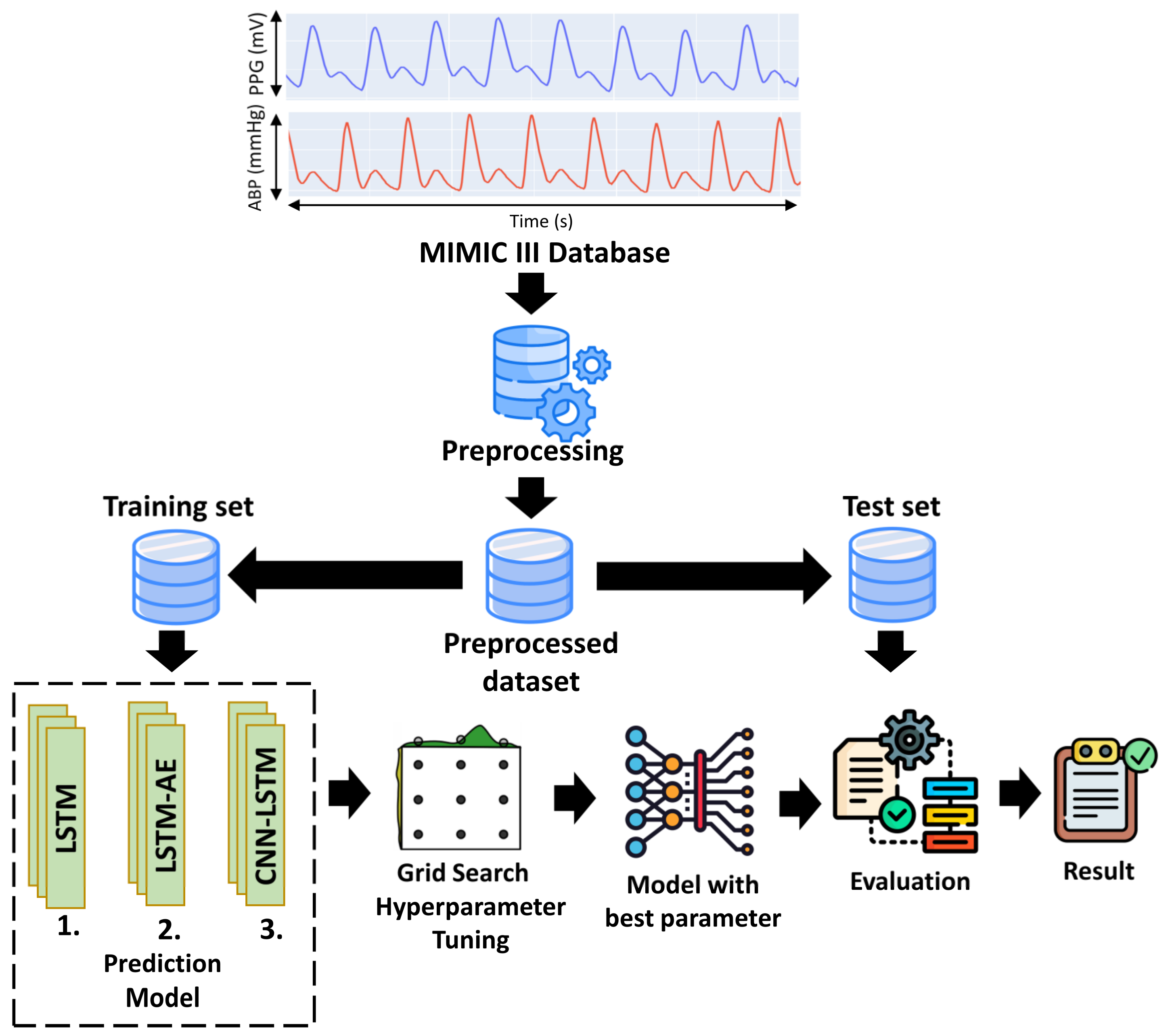
2. Materials and Methods
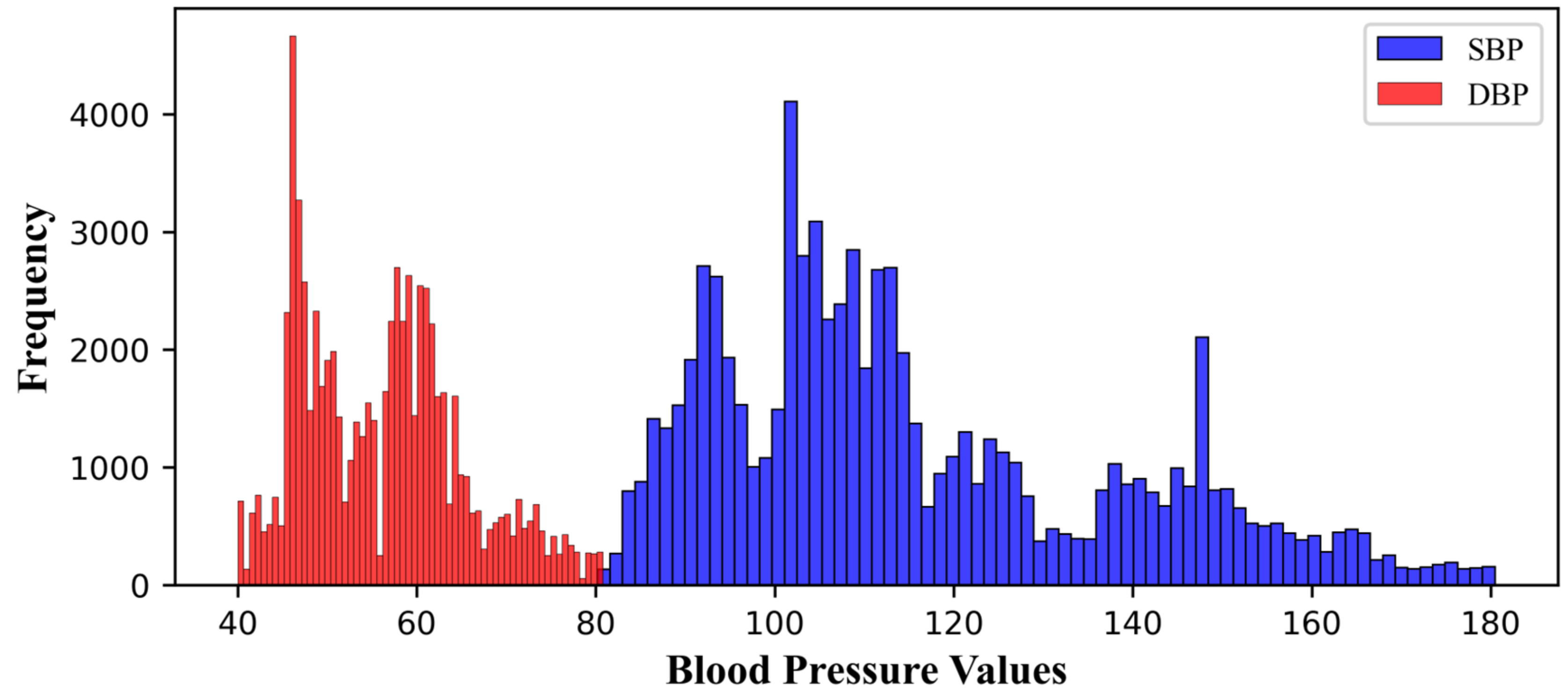
2.1. Dataset
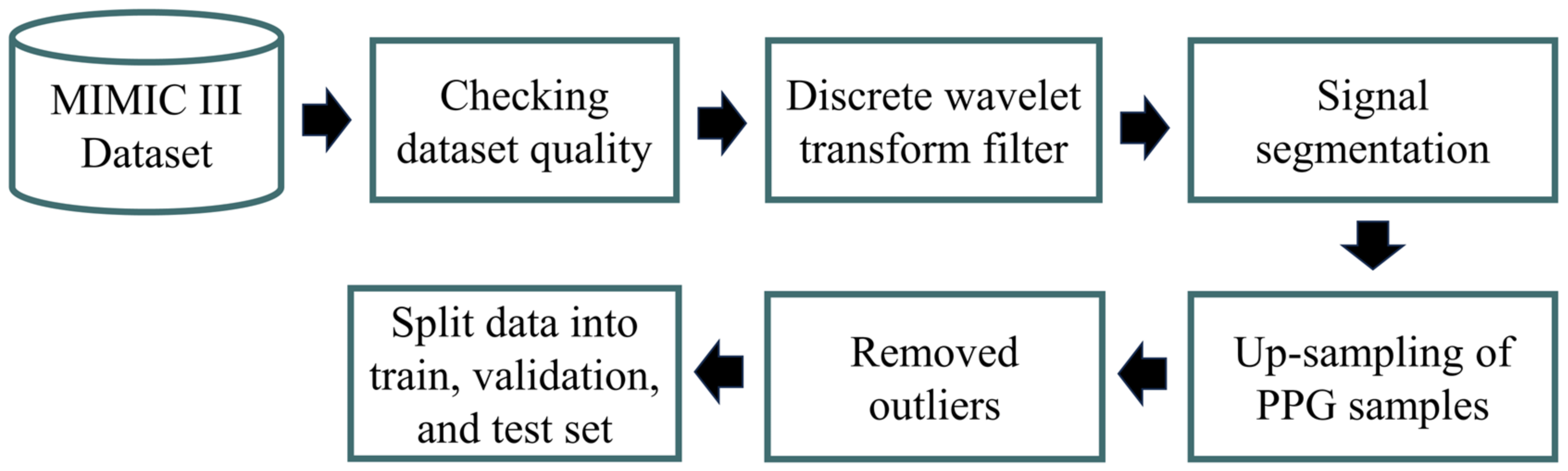
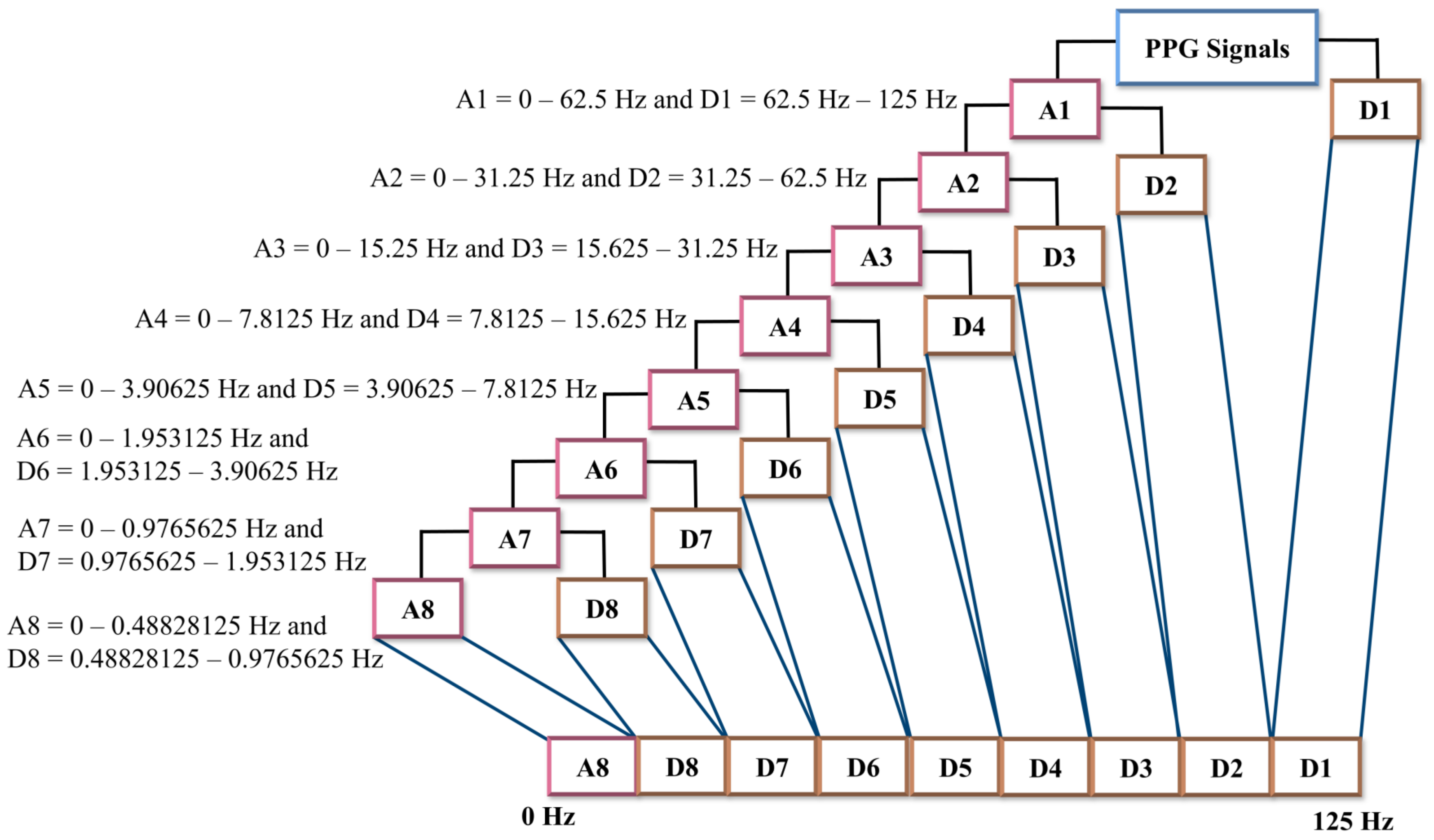
2.2. Preprocessing
2.3. Hyperparameters Tuning for the Proposed Model
Optimizer, Learning Rate, and Batch Size
- The stochastic gradient descent (SGD) optimizer updates the parameters iteratively by subtracting the gradient multiplied by the learning rate, as described in Equation (3):where is the update weight, the previous weight value, α is the learning rate, and is the gradient loss of function of which indicates the direction and magnitude of change required to optimize the model. The process described by this formula is repeated in the proposed deep learning simulation until the model reaches convergence or a state where the loss function is minimized and the prediction of the PPG dataset becomes optimal.
- b.
- Root mean square propagation (RMSprop): The RMSprop optimizer adapts the learning rate for each parameter based on the gradient changes in the previous iterations. RMSprop utilizes the average squared estimation of the previous gradients to adjust the learning rate at each parameter update step. The formula for RMSprop is described in Equations (4) and (5), where ρ represents the forgetting factor (set to 0.9) and t denotes the current time step:
- c.
- Adaptive moment estimation (Adam): Adam is the most commonly used optimization algorithm in deep learning for training models. The Adam optimizer combines momentum optimization concepts and RMSprop to effectively update model parameters during the training process. The Adam optimizer is widely employed in training deep learning models on time series datasets because it accelerates convergence and achieves superior results. The formula for the Adam optimizer is shown in Equation (6):and are the exponential decay rates, g is the gradient. By utilizing Formulae (6) and (7), the correct biases for the first and second moments can be calculated using Equations (8) and (9), respectively:
- d.
- Adadelta is an extension from AdaGrad, which is calculated by using Equation (12), where RMS is root mean square error:
2.4. Proposed Deep Learning Model for Estimating BP
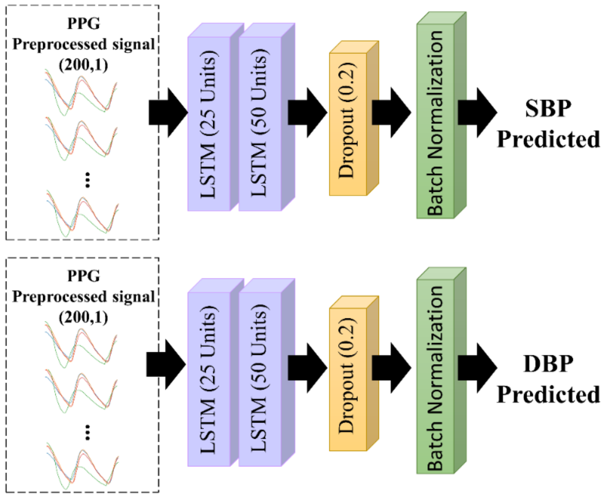
2.4.1. Long Short Term-Memory (LSTM) Architecture
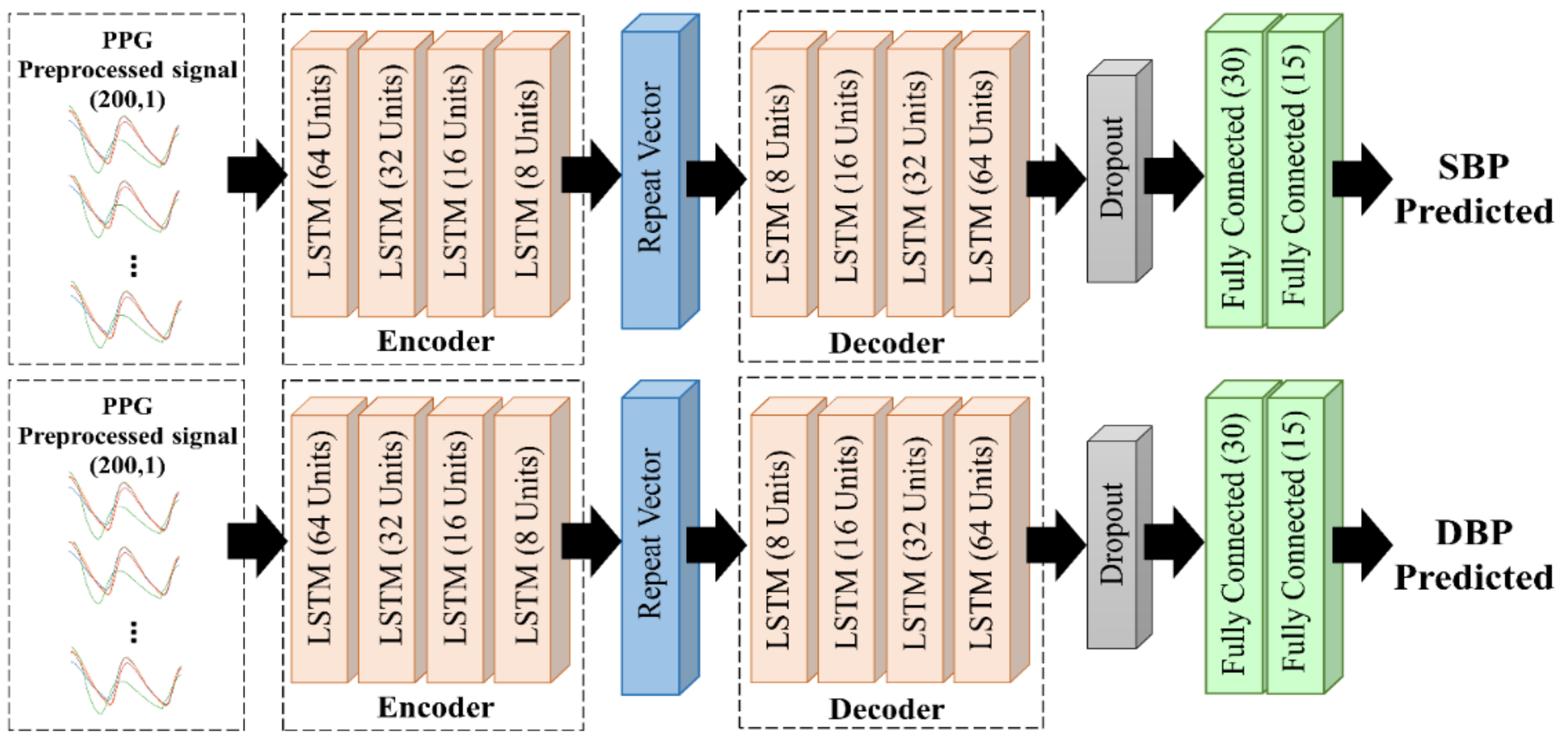
2.4.2. LSTM-Based Autoencoder
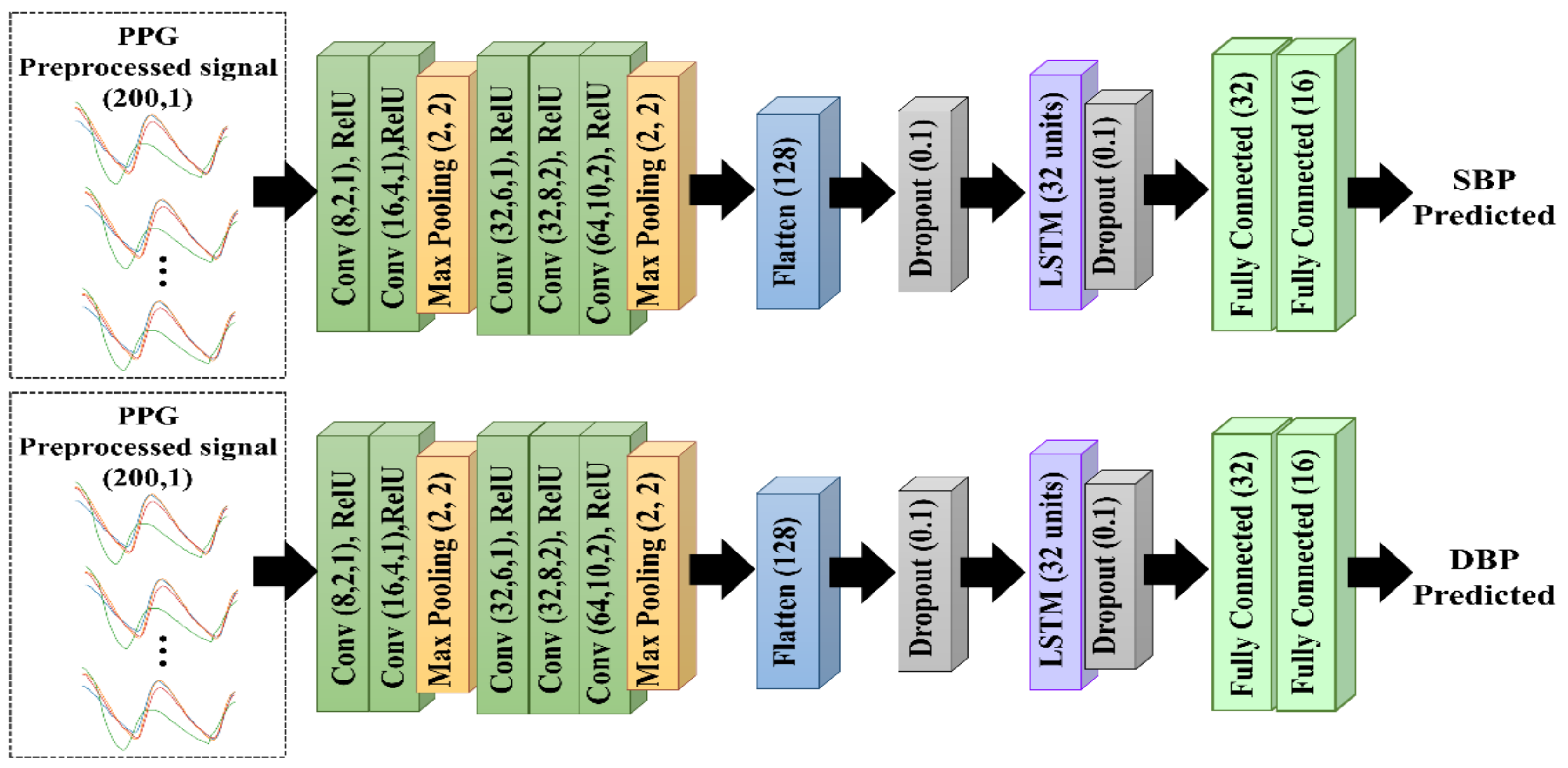
2.4.3. CNN–LSTM Architecture
2.5. Metrics and Evaluation
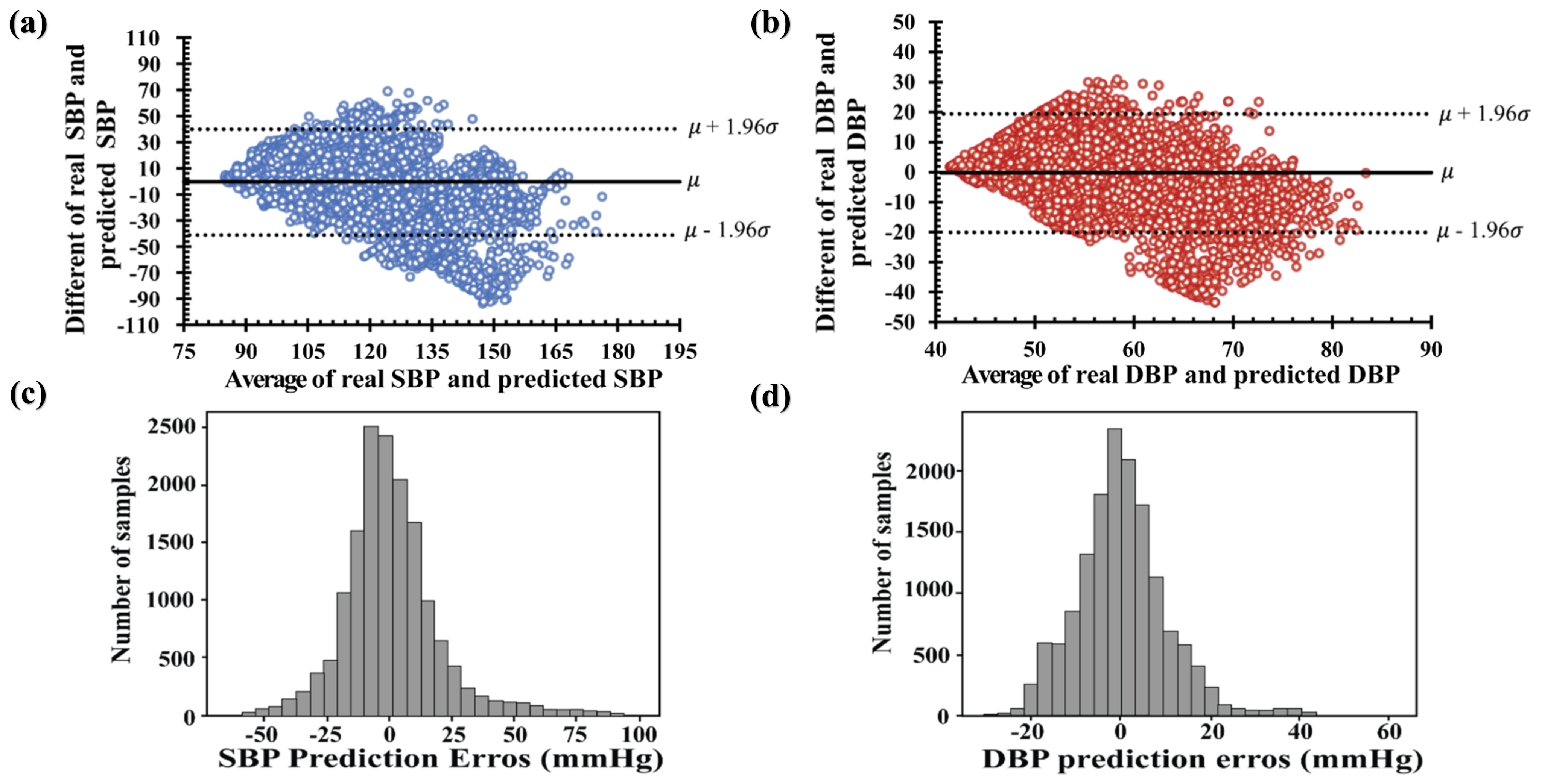
3. Results
4. Discussion
5. Conclusions
Author Contributions
Funding
Institutional Review Board Statement
Informed Consent Statement
Data Availability Statement
Conflicts of Interest
References
- Gupta, B. Monitoring in the ICU Anaesthesia Update. Updat. Anaethesia 2012, 28, 37–42. [Google Scholar]
- Martínez, G.; Howard, N.; Abbott, D.; Lim, K.; Ward, R.; Elgendi, M. Can Photoplethysmography Replace Arterial Blood Pressure in the Assessment of Blood Pressure? J. Clin. Med. 2018, 7, 316. [Google Scholar] [CrossRef] [Green Version]
- Allen, J. Photoplethysmography and Its Application in Clinical Physiological Measurement. Physiol. Meas. 2007, 28, R1–R39. [Google Scholar] [CrossRef] [PubMed] [Green Version]
- Elgendi, M.; Fletcher, R.; Liang, Y.; Howard, N.; Lovell, N.H.; Abbott, D.; Lim, K.; Ward, R. The Use of Photoplethysmography for Assessing Hypertension. NPJ Digit. Med. 2019, 2, 60. [Google Scholar] [CrossRef] [Green Version]
- Park, J.; Seok, H.S.; Kim, S.S.; Shin, H. Photoplethysmogram Analysis and Applications: An Integrative Review. Front. Physiol. 2022, 12, 808451. [Google Scholar] [CrossRef] [PubMed]
- Elgendi, M. On the Analysis of Fingertip Photoplethysmogram Signals. Curr. Cardiol. Rev. 2012, 8, 14–25. [Google Scholar] [CrossRef] [PubMed]
- Zhang, Y.; Feng, Z. A SVM Method for Continuous Blood Pressure Estimation from a PPG Signal. In Proceedings of the ACM International Conference Proceeding Series, Singapore, 24 February 2017; Association for Computing Machinery: New York, NY, USA, 2017; pp. 128–132. [Google Scholar]
- Hasanzadeh, N.; Ahmadi, M.M.; Mohammadzade, H. Blood Pressure Estimation Using Photoplethysmogram Signal and Its Morphological Features. IEEE Sens. J. 2020, 20, 4300–4310. [Google Scholar] [CrossRef]
- Samimi, H.; Dajani, H.R. Cuffless Blood Pressure Estimation Using Calibrated Cardiovascular Dynamics in the Photoplethysmogram. Bioengineering 2022, 9, 446. [Google Scholar] [CrossRef]
- Slapničar, G.; Mlakar, N.; Luštrek, M. Blood Pressure Estimation from Photoplethysmogram Using a Spectro-Temporal Deep Neural Network. Sensors 2019, 19, 3420. [Google Scholar] [CrossRef] [Green Version]
- Ibtehaz, N.; Mahmud, S.; Chowdhury, M.E.H.; Khandakar, A.; Khan, M.S.; Ayari, M.A.; Tahir, A.M.; Rahman, M.S. PPG2ABP: Translating Photoplethysmogram (PPG) Signals to Arterial Blood Pressure (ABP) Waveforms. Bioengineering 2022, 11, 692. [Google Scholar] [CrossRef]
- Aguirre, N.; Grall-Maës, E.; Cymberknop, L.J.; Armentano, R.L. Blood Pressure Morphology Assessment from Photoplethysmogram and Demographic Information Using Deep Learning with Attention Mechanism. Sensors 2021, 21, 2167. [Google Scholar] [CrossRef] [PubMed]
- Samimi, H.; Dajani, H.R. PPG-Based Calibration-Free Cuffless Blood Pressure Estimation Method Using Cardiovascular Dynamics. Sensors 2023, 23, 4145. [Google Scholar] [CrossRef] [PubMed]
- Shafiq, M.; Gu, Z. Deep Residual Learning for Image Recognition: A Survey. Appl. Sci. 2022, 12, 8972. [Google Scholar]
- Maeda-Gutiérrez, V.; Galván-Tejada, C.E.; Zanella-Calzada, L.A.; Celaya-Padilla, J.M.; Galván-Tejada, J.I.; Gamboa-Rosales, H.; Luna-García, H.; Magallanes-Quintanar, R.; Guerrero Méndez, C.A.; Olvera-Olvera, C.A. Comparison of Convolutional Neural Network Architectures for Classification of Tomato Plant Diseases. Appl. Sci. 2020, 10, 1245. [Google Scholar] [CrossRef] [Green Version]
- Li, Y.H.; Harfiya, L.N.; Chang, C.C. Featureless Blood Pressure Estimation Based on Photoplethysmography Signal Using CNN and BiLSTM for IoT Devices. Wirel. Commun. Mob. Comput. 2021, 2021, 9085100. [Google Scholar] [CrossRef]
- Alzubaidi, L.; Zhang, J.; Humaidi, A.J.; Al-Dujaili, A.; Duan, Y.; Al-Shamma, O.; Santamaría, J.; Fadhel, M.A.; Al-Amidie, M.; Farhan, L. Review of Deep Learning: Concepts, CNN Architectures, Challenges, Applications, Future Directions. J. Big Data 2021, 8, 53. [Google Scholar] [CrossRef]
- Johnson, A.E.W.; Pollard, T.J.; Shen, L.; Lehman, L.W.H.; Feng, M.; Ghassemi, M.; Moody, B.; Szolovits, P.; Anthony Celi, L.; Mark, R.G. MIMIC-III, a Freely Accessible Critical Care Database. Sci. Data 2016, 3, 160035. [Google Scholar] [CrossRef] [Green Version]
- Pollreisz, D.; TaheriNejad, N. Detection and Removal of Motion Artifacts in PPG Signals. Mob. Netw. Appl. 2022, 27, 728–738. [Google Scholar] [CrossRef] [Green Version]
- Polak, A.G.; Klich, B.; Saganowski, S.; Prucnal, M.A.; Kazienko, P. Processing Photoplethysmograms Recorded by Smartwatches to Improve the Quality of Derived Pulse Rate Variability. Sensors 2022, 22, 7047. [Google Scholar] [CrossRef]
- Jiang, H.; Zou, L.; Huang, D.; Feng, Q. Continuous Blood Pressure Estimation Based on Multi-Scale Feature Extraction by the Neural Network With Multi-Task Learning. Front. Neurosci. 2022, 16, 883693. [Google Scholar] [CrossRef]
- Fuadah, Y.N.; Pramudito, M.A.; Lim, K.M. An Optimal Approach for Heart Sound Classification Using Grid Search in Hyperparameter Optimization of Machine Learning. Bioengineering 2022, 10, 45. [Google Scholar] [CrossRef]
- Athaya, T.; Choi, S. An Estimation Method of Continuous Non-Invasive Arterial Blood Pressure Waveform Using Photoplethysmography: A u-Net Architecture-Based Approach. Sensors 2021, 21, 1867. [Google Scholar] [CrossRef]
- Ghosal, P.; Himavathi, S.; Srinivasan, E. PPG Motion Artifact Reduction Using Neural network and Spline Interpolation. In Proceedings of the IEEE 7th International Conference on Smart Structures and Systems ICSSS, Chennai, India, 23–24 July 2020; ISBN 9781728172231. [Google Scholar]
- Chobanian, A.V.; Bakris, G.L.; Black, H.R.; Cushman, W.C.; Green, L.A.; Izzo, J.L.; Jones, D.W.; Materson, B.J.; Oparil, S.; Wright, J.T.; et al. Seventh Report of the Joint National Committee on Prevention, Detection, Evaluation, and Treatment of High Blood Pressure. Hypertension 2003, 42, 1206–1252. [Google Scholar]
- Jiang, X.; Xu, C. Deep Learning and Machine Learning with Grid Search to Predict Later Occurrence of Breast Cancer Metastasis Using Clinical Data. J. Clin. Med. 2022, 11, 5772. [Google Scholar] [CrossRef]
- Ali, Y.A.; Awwad, E.M.; Al-Razgan, M.; Maarouf, A. Hyperparameter Search for Machine Learning Algorithms for Optimizing the Computational Complexity. Processes 2023, 11, 349. [Google Scholar] [CrossRef]
- Sun, S.; Cao, Z.; Zhu, H.; Zhao, J. A Survey of Optimization Methods from a Machine Learning Perspective. IEEE Trans. Cybern. 2019, 50, 3668–3681. [Google Scholar] [CrossRef] [Green Version]
- Uddin, M.J.; Li, Y.; Sattar, M.A.; Nasrin, Z.M.; Lu, C. Effects of Learning Rates and Optimization Algorithms on Forecasting Accuracy of Hourly Typhoon Rainfall: Experiments with Convolutional Neural Network. Earth Space Sci. 2022, 9, e2021EA002168. [Google Scholar] [CrossRef]
- Krizhevsky, A.; Sutskever, I.; Hinton, G.E. ImageNet Classification with Deep Convolutional Neural Networks. Commun. ACM 2017, 60, 84–90. [Google Scholar] [CrossRef] [Green Version]
- He, K.; Zhang, X.; Ren, S.; Sun, J. Deep Residual Learning for Image Recognition. In Proceedings of the IEEE Computer Society Conference on Computer Vision and Pattern Recognition, Las Vegas, NV, USA, 27–30 June 2016; IEEE Computer Society: Columbia, DC, USA, 2016; pp. 770–778. [Google Scholar]
- Usmani, I.A.; Qadri, M.T.; Zia, R.; Alrayes, F.S.; Saidani, O.; Dashtipour, K. Interactive Effect of Learning Rate and Batch Size to Implement Transfer Learning for Brain Tumor Classification. Electronics 2023, 12, 964. [Google Scholar] [CrossRef]
- Hassan, E.; Shams, M.Y.; Hikal, N.A.; Elmougy, S. The Effect of Choosing Optimizer Algorithms to Improve Computer Vision Tasks: A Comparative Study. Multimedia Tools Appl. 2022, 82, 16591–16633. [Google Scholar] [CrossRef]
- Wang, Y.; Liu, J.; Misic, J.; Misic, V.B.; Lv, S.; Chang, X. Assessing Optimizer Impact on DNN Model Sensitivity to Adversarial Examples. IEEE Access 2019, 7, 152766–152776. [Google Scholar] [CrossRef]
- Vysotskaya, N.; Will, C.; Servadei, L.; Maul, N.; Mandl, C.; Nau, M.; Harnisch, J.; Maier, A. Continuous Non-Invasive Blood Pressure Measurement Using 60 GHz-Radar—A Feasibility Study. Sensors 2023, 23, 4111. [Google Scholar] [CrossRef]
- Dogo, E.M.; Afolabi, O.J.; Twala, B. On the Relative Impact of Optimizers on Convolutional Neural Networks with Varying Depth and Width for Image Classification. Appl. Sci. 2022, 12, 11976. [Google Scholar] [CrossRef]
- Liu, M.; Yao, D.; Liu, Z.; Guo, J.; Chen, J. An Improved Adam Optimization Algorithm Combining Adaptive Coefficients and Composite Gradients Based on Randomized Block Coordinate Descent. Comput. Intell. Neurosci. 2023, 2023, 4765891. [Google Scholar] [CrossRef]
- Priyadarshini, I.; Cotton, C. A Novel LSTM–CNN–Grid Search-Based Deep Neural Network for Sentiment Analysis. J. Supercomput. 2021, 77, 13911–13932. [Google Scholar] [CrossRef]
- Glorot, X.; Bengio, Y. Understanding the Difficulty of Training Deep Feedforward Neural Networks. In Proceedings of the Thirteenth International Conference on Artificial Intelligence and Statistics, AISTATS 2010, Chia Laguna Resort, Sardinia, Italy, 13–15 May 2010. [Google Scholar]
- IEEE Standard Association. IEEE Standard for Wearable, Cuffless Blood Pressure Measuring Devices; IEEE Standards Committee: New York, NY, USA, 2014. [Google Scholar]
- O’brien, E.; Petrie, J.; Littler, W.; de Swiet, M.; Padfield, P.L.; Altmanu, D.G.; Blandg, M.; Coats, A.; Atkins, N. The British Hypertension Society Protocol for the Evaluation of Blood Pressure Measuring Devices. J. Hypertens. 1993, 11, S43–S62. [Google Scholar]
- White, W.B.; Berson, A.S.; Robbins, C.; Jamieson, M.J.; Prisant, L.M.; Roccella, E.; Sheps, S.G. Special Article National Standard for Measurement of Resting and Ambulatory Blood Pressures with Automated Sphygmomanometers. Hypertension 1993, 21, 504–509. [Google Scholar] [CrossRef] [Green Version]
- Qin, C.; Wang, X.; Xu, G.; Ma, X. Advances in Cuffless Continuous Blood Pressure Monitoring Technology Based on PPG Signals. Biomed. Res. Int. 2022, 2022, 8094351. [Google Scholar] [CrossRef]
- Liu, M.; Po, L.-M.; Fu, H. Cuffless Blood Pressure Estimation Based on Photoplethysmography Signal and Its Second Derivative. Int. J. Comput. Theory Eng. 2017, 9, 202–206. [Google Scholar] [CrossRef] [Green Version]
- Shimazaki, S.; Kawanaka, H.; Ishikawa, H.; Inoue, K.; Oguri, K. Cuffless Blood Pressure Estimation from Only the Waveform of Photoplethysmography Using CNN. In Proceedings of the 2019 41st Annual International Conference of the IEEE Engineering in Medicine and Biology Society (EMBC), Berlin, Germany, 23–27 July 2019; ISBN 9781538613115. [Google Scholar]
- Hochreiter, S.; Urgen Schmidhuber, J. Long Short-Term Memory. Neural Comput. 1997, 9, 1735–1780. [Google Scholar]


| BHS | Grade | CP | CP | CP | IEEE | Grade | MAD (mmHg) | AAMI | Grade | ME (mmHg) | SD (mmHg) |
| A | 60% | 85% | 95% | A | ≤5 | Pass | ≤5 | ≤8 | |||
| B | 50% | 75% | 90% | B | 5–6 | ||||||
| C | 40% | 65% | 85% | C | 6–7 | ||||||
| D | Lower than C | D | Lower than C | ||||||||
| Author | Method | Input | Dataset | SBP | DBP | ||
|---|---|---|---|---|---|---|---|
| MAE | SD | MAE | SD | ||||
| Proposed work | LSTM | PPG | MIMIC III | 14.2 | 20.7 | 7.53 | 10.01 |
| Proposed work | LSTM– Autoencoder | PPG | MIMIC III | 13.45 | 19.01 | 5.71 | 7.67 |
| Proposed work | CNN + LSTM | PPG | MIMIC III | 3.64 | 7.04 | 2.39 | 3.79 |
| [44] | SVR | PPG | MIMIC II | 8.54 | - | 4.34 | - |
| [7] | SVM | PPG | Queensland | 11.6 | 8.2 | 7.6 | 6.7 |
| [10] | Spectro-temporal ResNet | PPG | MIMIC III | 9.43 | - | 6.88 | - |
| [13] | ANN | PPG | MIMIC II | 9.74 | 12.40 | 4.65 | 6.29 |
| [12] | RNN | PPG | MIMIC III | 12.08 | 15.67 | 5.56 | 7.32 |
| [11] | U-Net | PPG | MIMIC III | 5.73 | - | 3.45 | - |
| [45] | CNN | PPG | Private dataset | - | 14.03 | - | - |
| [8] | AdaBoost | PPG | MIMIC II | 8.22 | 10.38 | 4.17 | 4.22 |
| [16] | CNN–BiLSTM | PPG | UCI (MIMIC II) | 7.85 | 8.41 | 4.42 | 4.80 |
| Assessment Evaluation | IEEE Standard | AAMI Standard | BHS Standards | ||||||
|---|---|---|---|---|---|---|---|---|---|
| MAD (≤4 mmHg) | MAPD (%) | Grade | ME (<5 mmHg) | SD (<8 mmHg) | CP5 (>60%) | CP10 (>85%) | CP15 (>95%) | Grade | |
| LSTM proposed model | |||||||||
| SBP | 14.281 | 0.12 | D | −0.49 | 20.7 | 30.92 | 53.07 | 67.37 | D |
| DBP | 7.53 | 0.133 | C | −0.21 | 10.01 | 45.14 | 72.02 | 86 | C |
| LSTM–autoencoder proposed model | |||||||||
| SBP | 26.94 | 0.11 | D | −0.93 | 19.01 | 27 | 52.5 | 68.70 | D |
| DBP | 5.71 | 0.01 | B | −0.56 | 7.67 | 56.67 | 83.8 | 92.98 | B |
| CNN–LSTM proposed model | |||||||||
| SBP | 5.34 | 0.04 | B | 0.13 | 7.04 | 63.4 | 85.9 | 92.78 | B |
| DBP | 2.89 | 0.05 | A | 0.48 | 3.79 | 81.70 | 98.28 | 100 | A |
Disclaimer/Publisher’s Note: The statements, opinions and data contained in all publications are solely those of the individual author(s) and contributor(s) and not of MDPI and/or the editor(s). MDPI and/or the editor(s) disclaim responsibility for any injury to people or property resulting from any ideas, methods, instructions or products referred to in the content. |
© 2023 by the authors. Licensee MDPI, Basel, Switzerland. This article is an open access article distributed under the terms and conditions of the Creative Commons Attribution (CC BY) license (https://creativecommons.org/licenses/by/4.0/).
Share and Cite
Mahardika T, N.Q.; Fuadah, Y.N.; Jeong, D.U.; Lim, K.M. PPG Signals-Based Blood-Pressure Estimation Using Grid Search in Hyperparameter Optimization of CNN–LSTM. Diagnostics 2023, 13, 2566. https://doi.org/10.3390/diagnostics13152566
Mahardika T NQ, Fuadah YN, Jeong DU, Lim KM. PPG Signals-Based Blood-Pressure Estimation Using Grid Search in Hyperparameter Optimization of CNN–LSTM. Diagnostics. 2023; 13(15):2566. https://doi.org/10.3390/diagnostics13152566
Chicago/Turabian StyleMahardika T, Nurul Qashri, Yunendah Nur Fuadah, Da Un Jeong, and Ki Moo Lim. 2023. "PPG Signals-Based Blood-Pressure Estimation Using Grid Search in Hyperparameter Optimization of CNN–LSTM" Diagnostics 13, no. 15: 2566. https://doi.org/10.3390/diagnostics13152566