
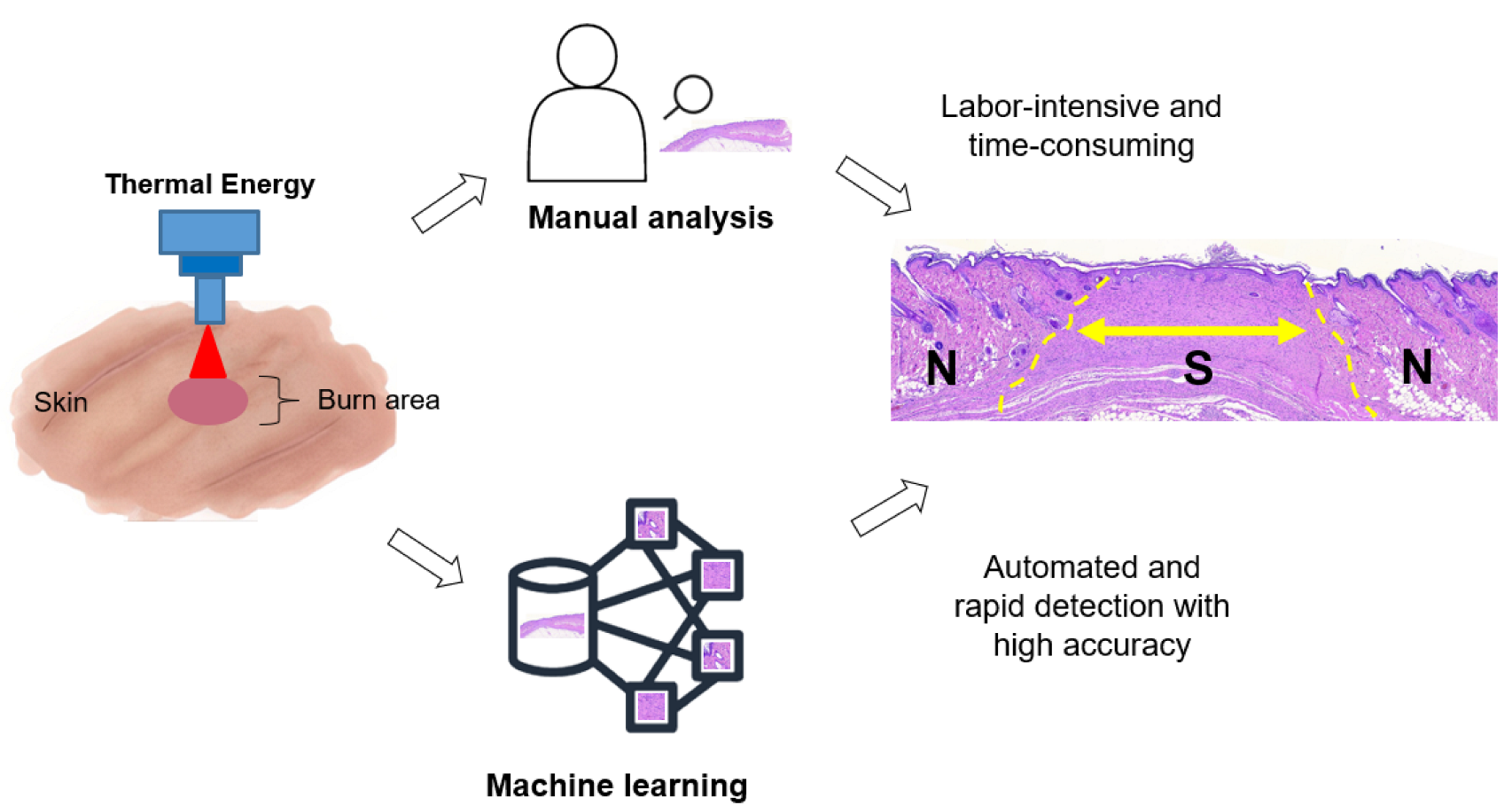
Automated Structural Analysis and Quantitative Characterization of Scar Tissue Using Machine Learning

 , and
, and
Abstract
:1. Introduction
2. Materials and Methods
2.1. In Vivo Scar Model
2.2. Histology Preparation
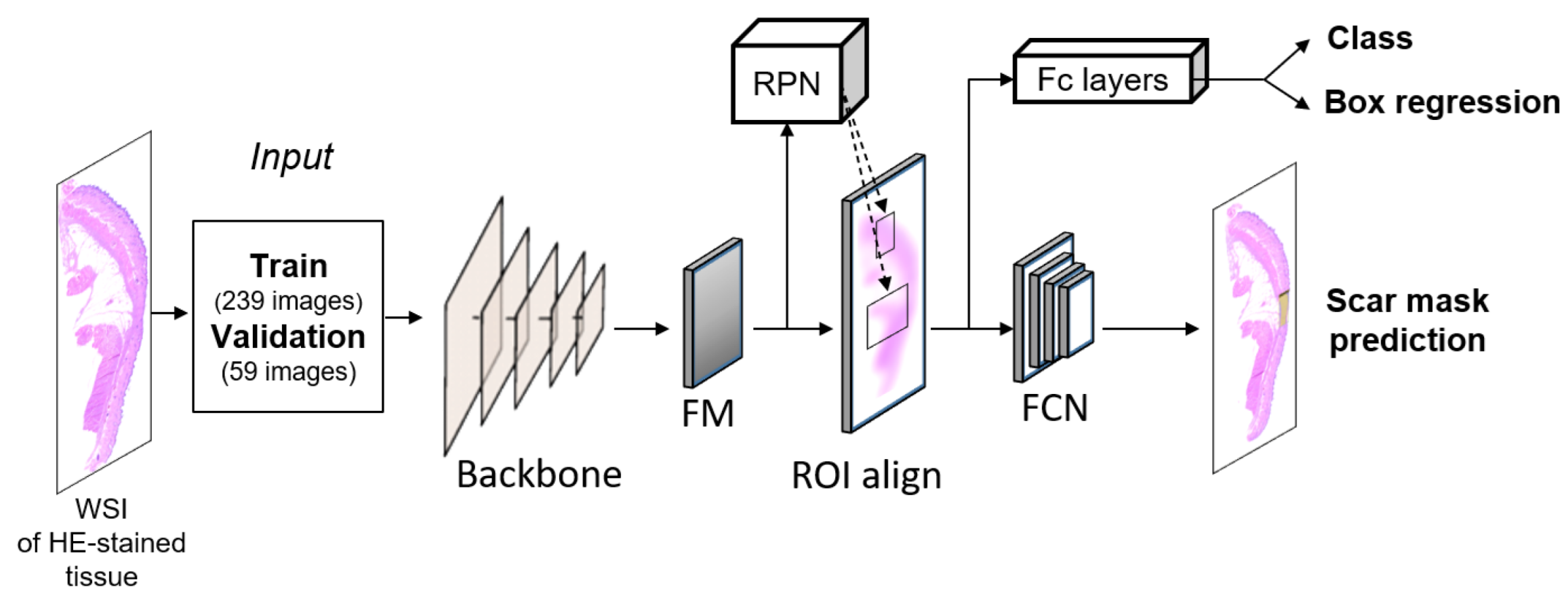
2.3. Scar Recognition: Mask Region-Based Convolutional Neural Network (RCNN)
2.4. Machine Learning
2.5. Evaluation Metrics
2.6. Scar Extraction
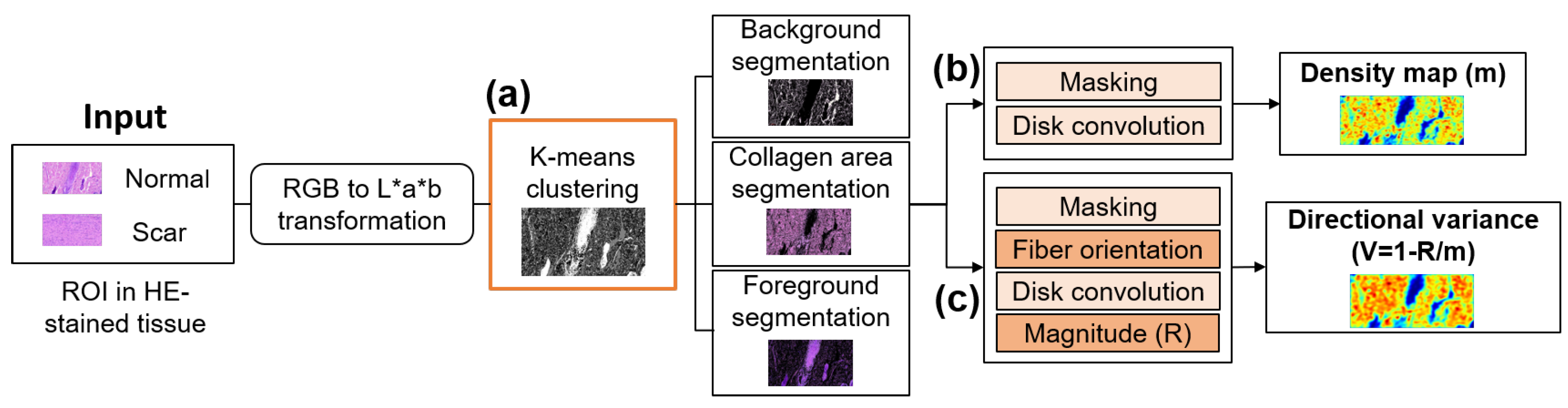
2.7. Tissue Segmentation: K-Means Clustering
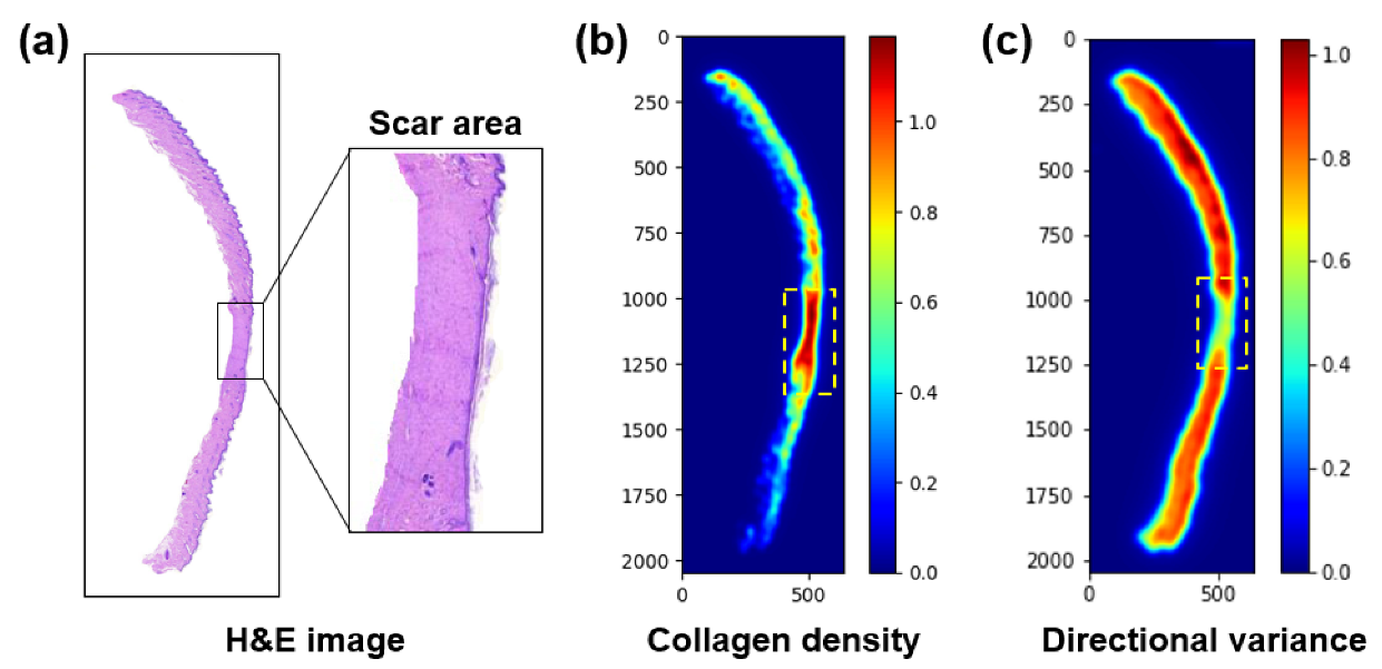
2.8. Collagen Density and Directional Variance of Collagen
2.9. Statistical Analysis
3. Results
3.1. Scar Recognition
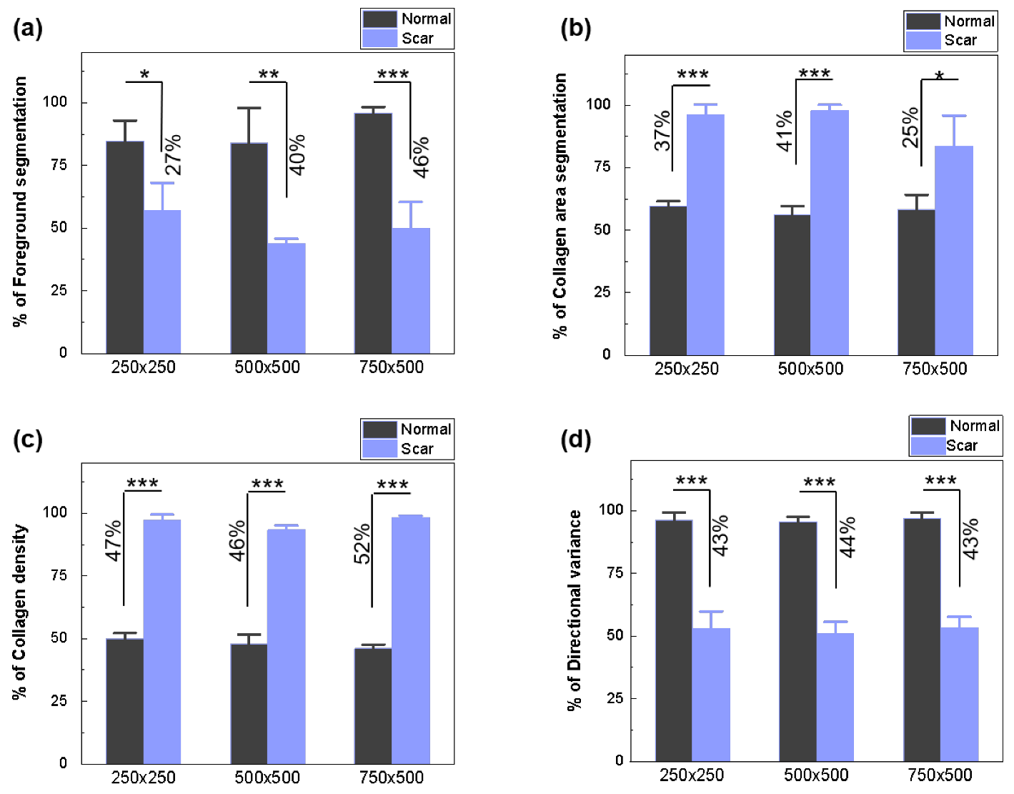
3.2. Scar Characterization
4. Discussion
5. Conclusions
Author Contributions
Funding
Institutional Review Board Statement
Informed Consent Statement
Conflicts of Interest
Abbreviations
| HE | Hematoxylin and eosin |
| WSI | Whole slide image |
| SHG | Second harmonic generation |
| MT | Masson’s trichrome |
| CNN | Convolutional neural network |
| RCNN | Region-based CNN |
| RPN | Region proposal network |
| ANOVA | Analysis of variance |
| ROI | region of interest |
| CAS | Collagen area segmentation |
| CDM | Collagen density map |
| DV | Directional variance |
| AI | Artificial intelligence |
| FS | Foreground segmentation |
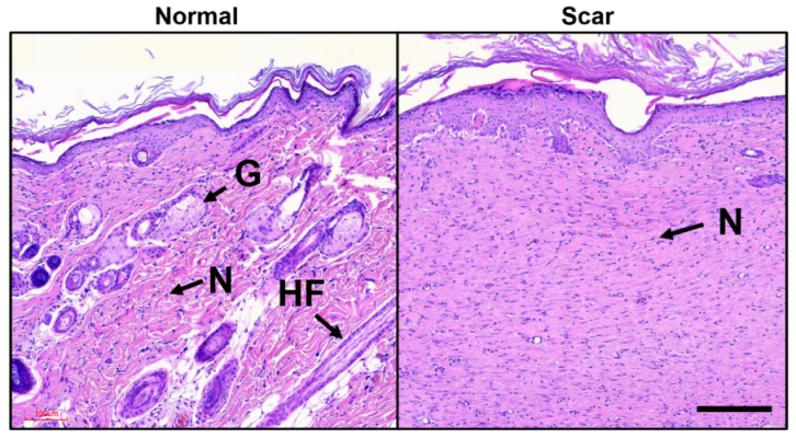
| HF | Hair follicle |
| G | Gland |
| N | Nuclei |
References
- Chow, L.; Yick, K.L.; Sun, Y.; Leung, M.S.; Kwan, M.Y.; Ng, S.P.; Yu, A.; Yip, J.; Chan, Y.F. A Novel Bespoke Hypertrophic Scar Treatment: Actualizing Hybrid Pressure and Silicone Therapies with 3D Printing and Scanning. Int. J. Bioprint. 2021, 7, 327. [Google Scholar] [CrossRef] [PubMed]
- Liu, X.G.; Zhang, D. Evaluation of efficacy of corticosteroid and corticosteroid combined with botulinum toxin type A in the treatment of keloid and hypertrophic scars: A meta-analysis. Aesthetic Plast. Surg. 2021, 45, 3037–3044. [Google Scholar] [CrossRef] [PubMed]
- Salem, S.A.M.; Abdel Hameed, S.M.; Mostafa, A.E. Intense pulsed light versus cryotherapy in the treatment of hypertrophic scars: A clinical and histopathological study. J. Cosmet. Dermatol. 2021, 20, 2775–2784. [Google Scholar] [CrossRef] [PubMed]
- Zhang, Y.; Wang, Z.; Mao, Y. RPN Prototype Alignment for Domain Adaptive Object Detector. In Proceedings of the IEEE/CVF Conference on Computer Vision and Pattern Recognition, Nashville, TN, USA, 20–25 June 2021; pp. 12425–12434. [Google Scholar]
- Machado, B.H.B.; Zhang, J.; Frame, J.; Najlah, M. Treatment of Scars with Laser-Assisted Delivery of Growth Factors and Vitamin C: A Comparative, Randomised, Double-blind, Early Clinical Trial. Aesthetic Plast. Surg. 2021, 45, 2363–2374. [Google Scholar] [CrossRef]
- Fayzullin, A.; Ignatieva, N.; Zakharkina, O.; Tokarev, M.; Mudryak, D.; Khristidis, Y.; Balyasin, M.; Kurkov, A.; Churbanov, S.; Dyuzheva, T. Modeling of Old Scars: Histopathological, Biochemical and Thermal Analysis of the Scar Tissue Maturation. Biology 2021, 10, 136. [Google Scholar] [CrossRef]
- Huang, T.Y.; Wang, Z.Z.; Gong, Y.F.; Liu, X.C.; Zhang, X.M.; Huang, X.Y. Scar-reducing effects of gambogenic acid on skin wounds in rabbit ears. Int. Immunopharmacol. 2021, 90, 107200. [Google Scholar]
- Hsu, W.C.; Spilker, M.H.; Yannas, I.V.; Rubin, P.A.D. Inhibition of conjunctival scarring and contraction by a porous collagen-glycosaminoglycan implant. Investig. Ophthalmol. Vis. Sci. 2000, 41, 2404–2411. [Google Scholar]
- Limandjaja, G.C.; van den Broek, L.J.; Waaijman, T.; van Veen, H.A.; Everts, V.; Monstrey, S.; Scheper, R.J.; Niessen, F.B.; Gibbs, S. Increased epidermal thickness and abnormal epidermal differentiation in keloid scars. Br. J. Dermatol. 2017, 176, 116–126. [Google Scholar] [CrossRef] [Green Version]
- Sivaguru, M.; Durgam, S.; Ambekar, R.; Luedtke, D.; Fried, G.; Stewart, A.; Toussaint, K.C. Quantitative analysis of collagen fiber organization in injured tendons using Fourier transform-second harmonic generation imaging. Opt. Express 2010, 18, 24983–24993. [Google Scholar] [CrossRef]
- Yang, S.W.; Geng, Z.J.; Ma, K.; Sun, X.Y.; Fu, X.B. Comparison of the histological morphology between normal skin and scar tissue. J. Huazhong Univ. Sci. Technol. Med. Sci. 2016, 36, 265–269. [Google Scholar] [CrossRef]
- Mostaço-Guidolin, L.; Rosin, N.L.; Hackett, T.L. Imaging collagen in scar tissue: Developments in second harmonic generation microscopy for biomedical applications. Int. J. Mol. Sci. 2017, 18, 1772. [Google Scholar] [CrossRef] [PubMed]
- Wang, Q.; Liu, W.; Chen, X.; Wang, X.; Chen, G.; Zhu, X. Quantification of scar collagen texture and prediction of scar development via second harmonic generation images and a generative adversarial network. Biomed. Opt. Express 2021, 12, 5305–5319. [Google Scholar] [CrossRef] [PubMed]
- Bayan, C.; Levitt, J.M.; Miller, E.; Kaplan, D.; Georgakoudi, I. Fully automated, quantitative, noninvasive assessment of collagen fiber content and organization in thick collagen gels. J. Appl. Phys. 2009, 105, 102042. [Google Scholar] [CrossRef] [PubMed]
- Clift, C.L.; Su, Y.R.; Bichell, D.; Smith, H.C.J.; Bethard, J.R.; Norris-Caneda, K.; Comte-Walters, S.; Ball, L.E.; Hollingsworth, M.A.; Mehta, A.S. Collagen fiber regulation in human pediatric aortic valve development and disease. Sci. Rep. 2021, 11, 9751. [Google Scholar] [CrossRef]
- Fereidouni, F.; Todd, A.; Li, Y.; Chang, C.W.; Luong, K.; Rosenberg, A.; Lee, Y.J.; Chan, J.W.; Borowsky, A.; Matsukuma, K. Dual-mode emission and transmission microscopy for virtual histochemistry using hematoxylin-and eosin-stained tissue sections. Biomed. Opt. Express 2019, 10, 6516–6530. [Google Scholar] [CrossRef]
- Coelho, P.G.B.; de Souza, M.V.; Conceição, L.G.; Viloria, M.I.V.; Bedoya, S.A.O. Evaluation of dermal collagen stained with picrosirius red and examined under polarized light microscopy. An. Bras. De Dermatol. 2018, 93, 415–418. [Google Scholar] [CrossRef] [Green Version]
- Suvik, A.; Effendy, A.W.M. The use of modified Masson’s trichrome staining in collagen evaluation in wound healing study. Mal. J. Vet. Res. 2012, 3, 39–47. [Google Scholar]
- Rieppo, L.; Janssen, L.; Rahunen, K.; Lehenkari, P.; Finnilä, M.A.J.; Saarakkala, S. Histochemical quantification of collagen content in articular cartilage. PLoS ONE 2019, 14, e0224839. [Google Scholar] [CrossRef] [Green Version]
- Tanaka, R.; Fukushima, S.i.; Sasaki, K.; Tanaka, Y.; Murota, H.; Matsumoto, K.; Araki, T.; Yasui, T. In vivo visualization of dermal collagen fiber in skin burn by collagen-sensitive second-harmonic-generation microscopy. J. Biomed. Opt. 2013, 18, 061231. [Google Scholar] [CrossRef]
- Pham, T.T.A.; Kim, H.; Lee, Y.; Kang, H.W.; Park, S. Deep Learning for Analysis of Collagen Fiber Organization in Scar Tissue. IEEE Access 2021, 9, 101755–101764. [Google Scholar] [CrossRef]
- Erickson, B.J.; Korfiatis, P.; Akkus, Z.; Kline, T.L. Machine learning for medical imaging. Radiographics 2017, 37, 505–515. [Google Scholar] [CrossRef] [PubMed]
- Rajula, H.S.R.; Verlato, G.; Manchia, M.; Antonucci, N.; Fanos, V. Comparison of conventional statistical methods with machine learning in medicine: Diagnosis, drug development, and treatment. Medicina 2020, 56, 455. [Google Scholar] [CrossRef] [PubMed]
- Li, M.; Cheng, Y.; Zhao, H. Unlabeled data classification via support vector machines and k-means clustering. In Proceedings of the International Conference on Computer Graphics, Imaging and Visualization, 2004. CGIV 2004, Penang, Malaysia, 2 July 2004; pp. 183–186. [Google Scholar]
- Yamashita, R.; Nishio, M.; Do, R.K.G.; Togashi, K. Convolutional neural networks: An overview and application in radiology. Insights Imaging 2018, 9, 611–629. [Google Scholar] [CrossRef] [PubMed] [Green Version]
- Hashemzehi, R.; Mahdavi, S.J.S.; Kheirabadi, M.; Kamel, S.R. Detection of brain tumors from MRI images base on deep learning using hybrid model CNN and NADE. Biocybern. Biomed. Eng. 2020, 40, 1225–1232. [Google Scholar] [CrossRef]
- Bhatt, A.R.; Ganatra, A.; Kotecha, K. Cervical cancer detection in pap smear whole slide images using convnet with transfer learning and progressive resizing. PeerJ Comput. Sci. 2021, 7, e348. [Google Scholar] [CrossRef]
- Johnson, J.W. Adapting mask-rcnn for automatic nucleus segmentation. arXiv 2018, arXiv:1805.00500. [Google Scholar]
- Ghiasi, G.; Lin, T.Y.; Le, Q.V. Nas-fpn: Learning scalable feature pyramid architecture for object detection. In Proceedings of the IEEE/CVF Conference on Computer Vision and Pattern Recognition, Long Beach, CA, USA, 15–20 June 2019; pp. 7036–7045. [Google Scholar]
- Kim, M.; Kim, S.W.; Kim, H.; Hwang, C.W.; Choi, J.M.; Kang, H.W. Development of a reproducible in vivo laser-induced scar model for wound healing study and management. Biomed. Opt. Express 2019, 10, 1965–1977. [Google Scholar] [CrossRef]
- He, K.; Gkioxari, G.; Dollár, P.; Girshick, R. Mask r-cnn. In Proceedings of the IEEE International Conference on Computer Vision, Venice, Italy, 22–29 October 2017; pp. 2961–2969. [Google Scholar]
- Kim, Y.; Park, H. Deep learning-based automated and universal bubble detection and mask extraction in complex two-phase flows. Sci. Rep. 2021, 11, 8940. [Google Scholar] [CrossRef]
- Chen, K.; Wang, J.; Pang, J.; Cao, Y.; Xiong, Y.; Li, X.; Sun, S.; Feng, W.; Liu, Z.; Xu, J. MMDetection: Open mmlab detection toolbox and benchmark. arXiv 2019, arXiv:1906.07155. [Google Scholar]
- Amjoud, A.B.; Amrouch, M. Convolutional neural networks backbones for object detection. In International Conference on Image and Signal Processing; Springer: Berlin/Heidelberg, Germany, 2020; pp. 282–289. [Google Scholar]
- Lin, T.Y.; Dollár, P.; Girshick, R.; He, K.; Hariharan, B.; Belongie, S. Feature pyramid networks for object detection. In Proceedings of the IEEE Conference on Computer Vision and Pattern Recognition, Honolulu, HI, USA, 21–26 July 2017; pp. 2117–2125. [Google Scholar]
- Jaiswal, A.; Wu, Y.; Natarajan, P.; Natarajan, P. Class-agnostic object detection. In Proceedings of the IEEE/CVF Winter Conference on Applications of Computer Vision, Waikola, HI, USA, 5–9 January 2021; pp. 919–928. [Google Scholar]
- Varadarajan, V.; Garg, D.; Kotecha, K. An Efficient Deep Convolutional Neural Network Approach for Object Detection and Recognition Using a Multi-Scale Anchor Box in Real-Time. Future Internet 2021, 13, 307. [Google Scholar] [CrossRef]
- Garg, D.; Jain, P.; Kotecha, K.; Goel, P.; Varadarajan, V. An Efficient Multi-Scale Anchor Box Approach to Detect Partial Faces from a Video Sequence. Big Data Cogn. Comput. 2022, 6, 9. [Google Scholar] [CrossRef]
- Chaudhari, P.; Agrawal, H.; Kotecha, K. Data augmentation using MG-GAN for improved cancer classification on gene expression data. Soft Comput. 2020, 24, 11381–11391. [Google Scholar] [CrossRef]
- Kozlov, A. Working with scale: 2nd place solution to Product Detection in Densely Packed Scenes [Technical Report]. arXiv 2020, arXiv:2006.07825. [Google Scholar]
- Cetinic, E.; Lipic, T.; Grgic, S. Fine-tuning convolutional neural networks for fine art classification. Expert Syst. Appl. 2018, 114, 107–118. [Google Scholar] [CrossRef]
- Rukmangadha, P.V.; Das, R. Representation-Learning-Based Fusion Model for Scene Classification Using Convolutional Neural Network (CNN) and Pre-trained CNNs as Feature Extractors. In Computational Intelligence in Pattern Recognition; Springer: Berlin/Heidelberg, Germany, 2022; pp. 631–643. [Google Scholar]
- Shaodan, L.; Chen, F.; Zhide, C. A ship target location and mask generation algorithms base on Mask RCNN. Int. J. Comput. Intell. Syst. 2019, 12, 1134–1143. [Google Scholar] [CrossRef] [Green Version]
- Neumann, L.; Zisserman, A.; Vedaldi, A. Relaxed Softmax: Efficient Confidence Auto-Calibration for Safe Pedestrian Detection. 2018. Available online: https://openreview.net/forum?id=S1lG7aTnqQ (accessed on 22 July 2021).
- WS, R. Imagej, US National Institutes of Health, Bethesda, Maryland, USA. 2009. Available online: http://rsb.info.nih.gov/ij/ (accessed on 5 August 2021).
- Kaur, A.; Kranthi, B.V. Comparison between YCbCr color space and CIELab color space for skin color segmentation. Int. J. Appl. Inf. Syst. 2012, 3, 30–33. [Google Scholar]
- Dey, R.; Roy, K.; Bhattacharjee, D.; Nasipuri, M.; Ghosh, P. An Automated system for Segmenting platelets from Microscopic images of Blood Cells. In Proceedings of the 2015 International Symposium on Advanced Computing and Communication (ISACC), Silchar, India, 14–15 September 2015; pp. 230–237. [Google Scholar]
- Quinn, K.P.; Golberg, A.; Broelsch, G.F.; Khan, S.; Villiger, M.; Bouma, B.; Austen, W.G., Jr.; Sheridan, R.L.; Mihm, M.C., Jr.; Yarmush, M.L. An automated image processing method to quantify collagen fibre organization within cutaneous scar tissue. Exp. Dermatol. 2015, 24, 78–80. [Google Scholar] [CrossRef] [Green Version]
- Quinn, K.P.; Georgakoudi, I. Rapid quantification of pixel-wise fiber orientation data in micrographs. J. Biomed. Opt. 2013, 18, 46003. [Google Scholar] [CrossRef] [Green Version]
- Ivasic-Kos, M.; Pobar, M. Building a labeled dataset for recognition of handball actions using mask R-CNN and STIPS. In Proceedings of the 2018 7th European Workshop on Visual Information Processing (EUVIP), Tampere, Finland, 26–28 November 2018; pp. 1–6. [Google Scholar]
- Qin, Z.; Li, Z.; Zhang, Z.; Bao, Y.; Yu, G.; Peng, Y.; Sun, J. ThunderNet: Towards real-time generic object detection on mobile devices. In Proceedings of the IEEE/CVF International Conference on Computer Vision, Seoul, Korea, 27–28 October 2019; pp. 6718–6727. [Google Scholar]
- Bautista, P.A.; Abe, T.; Yamaguchi, M.; Yagi, Y.; Ohyama, N. Digital staining for multispectral images of pathological tissue specimens based on combined classification of spectral transmittance. Comput. Med. Imaging Graph. 2005, 29, 649–657. [Google Scholar] [CrossRef]
- Zhang, C.; Yin, K.; Shen, Y.m. Efficacy of fractional carbon dioxide laser therapy for burn scars: A meta-analysis. J. Dermatol. Treat. 2021, 32, 845–850. [Google Scholar] [CrossRef]
- Sarwinda, D.; Paradisa, R.H.; Bustamam, A.; Anggia, P. Deep Learning in Image Classification using Residual Network (ResNet) Variants for Detection of Colorectal Cancer. Procedia Comput. Sci. 2021, 179, 423–431. [Google Scholar] [CrossRef]
- He, K.; Zhang, X.; Ren, S.; Sun, J. Deep residual learning for image recognition. In Proceedings of the IEEE Conference on Computer Vision and Pattern Recognition, Las Vegas, NV, USA, 27–30 June 2016; pp. 770–778. [Google Scholar]
- Zhang, H.; Wu, C.; Zhang, Z.; Zhu, Y.; Lin, H.; Zhang, Z.; Sun, Y.; He, T.; Mueller, J.; Manmatha, R. Resnest: Split-attention networks. arXiv 2020, arXiv:2004.08955. [Google Scholar]
- Mehl, A.A.; Schneider, B.; Schneider, F.K.; Carvalho, B.H.K.D. Measurement of wound area for early analysis of the scar predictive factor. Rev. Lat.-Am. Enferm. 2020, 28. [Google Scholar] [CrossRef] [PubMed]
- Shi, P.; Zhong, J.; Huang, R.; Lin, J. Automated quantitative image analysis of hematoxylin-eosin staining slides in lymphoma based on hierarchical Kmeans clustering. In Proceedings of the 2016 8th International Conference on Information Technology in Medicine and Education (ITME), Fuzhou, China, 23–25 December 2016; pp. 99–104. [Google Scholar]
- Osman, O.S.; Selway, J.L.; Harikumar, P.E.; Jassim, S.; Langlands, K. Automated Analysis of Collagen Histology in Ageing Skin. In BIOIMAGING; SCITEPRESS—Science and Technology Publications, Lda: Angers, France, 2014; pp. 41–48. [Google Scholar]


| Hyperparameter | Configuration |
|---|---|
| Optimizer | Stochastic gradient descent (SGD) |
| Learning rate | 0.0025 |
| Epoch | 600 |
| batch size | 2 |
| Backbone | Time (s) | ||||
|---|---|---|---|---|---|
| ResNet 50 | 0.598 | 0.666 | 0.619 | 0.672 | 0.05 |
| ResNet 101 | 0.620 | 0.680 | 0.631 | 0.677 | 0.07 |
| ResNeSt 50 | 0.564 | 0.641 | 0.613 | 0.659 | 0.07 |
| ResNest 101 | 0.597 | 0.672 | 0.587 | 0.645 | 0.09 |
Publisher’s Note: MDPI stays neutral with regard to jurisdictional claims in published maps and institutional affiliations. |
© 2022 by the authors. Licensee MDPI, Basel, Switzerland. This article is an open access article distributed under the terms and conditions of the Creative Commons Attribution (CC BY) license (https://creativecommons.org/licenses/by/4.0/).
Share and Cite
Maknuna, L.; Kim, H.; Lee, Y.; Choi, Y.; Kim, H.; Yi, M.; Kang, H.W. Automated Structural Analysis and Quantitative Characterization of Scar Tissue Using Machine Learning. Diagnostics 2022, 12, 534. https://doi.org/10.3390/diagnostics12020534
Maknuna L, Kim H, Lee Y, Choi Y, Kim H, Yi M, Kang HW. Automated Structural Analysis and Quantitative Characterization of Scar Tissue Using Machine Learning. Diagnostics. 2022; 12(2):534. https://doi.org/10.3390/diagnostics12020534
Chicago/Turabian StyleMaknuna, Luluil, Hyeonsoo Kim, Yeachan Lee, Yoonjin Choi, Hyunjung Kim, Myunggi Yi, and Hyun Wook Kang. 2022. "Automated Structural Analysis and Quantitative Characterization of Scar Tissue Using Machine Learning" Diagnostics 12, no. 2: 534. https://doi.org/10.3390/diagnostics12020534