Comparison between Statistical Models and Machine Learning Methods on Classification for Highly Imbalanced Multiclass Kidney Data

 ,
,
Abstract
:1. Introduction
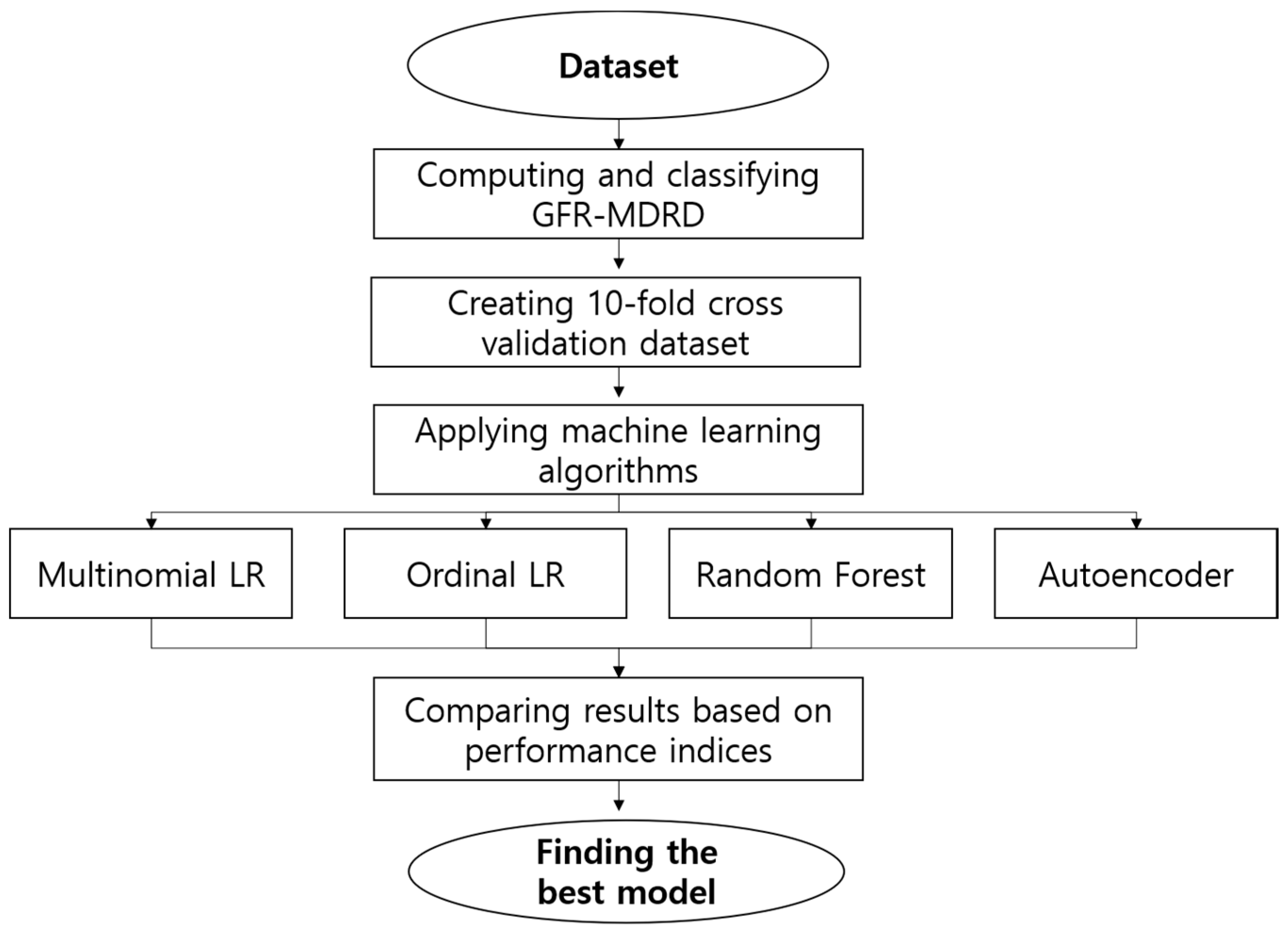
2. Methods and Materials
2.1. Methods
2.1.1. Multinomial Logistic Regression Model
2.1.2. Ordinal Logistic Regression Model
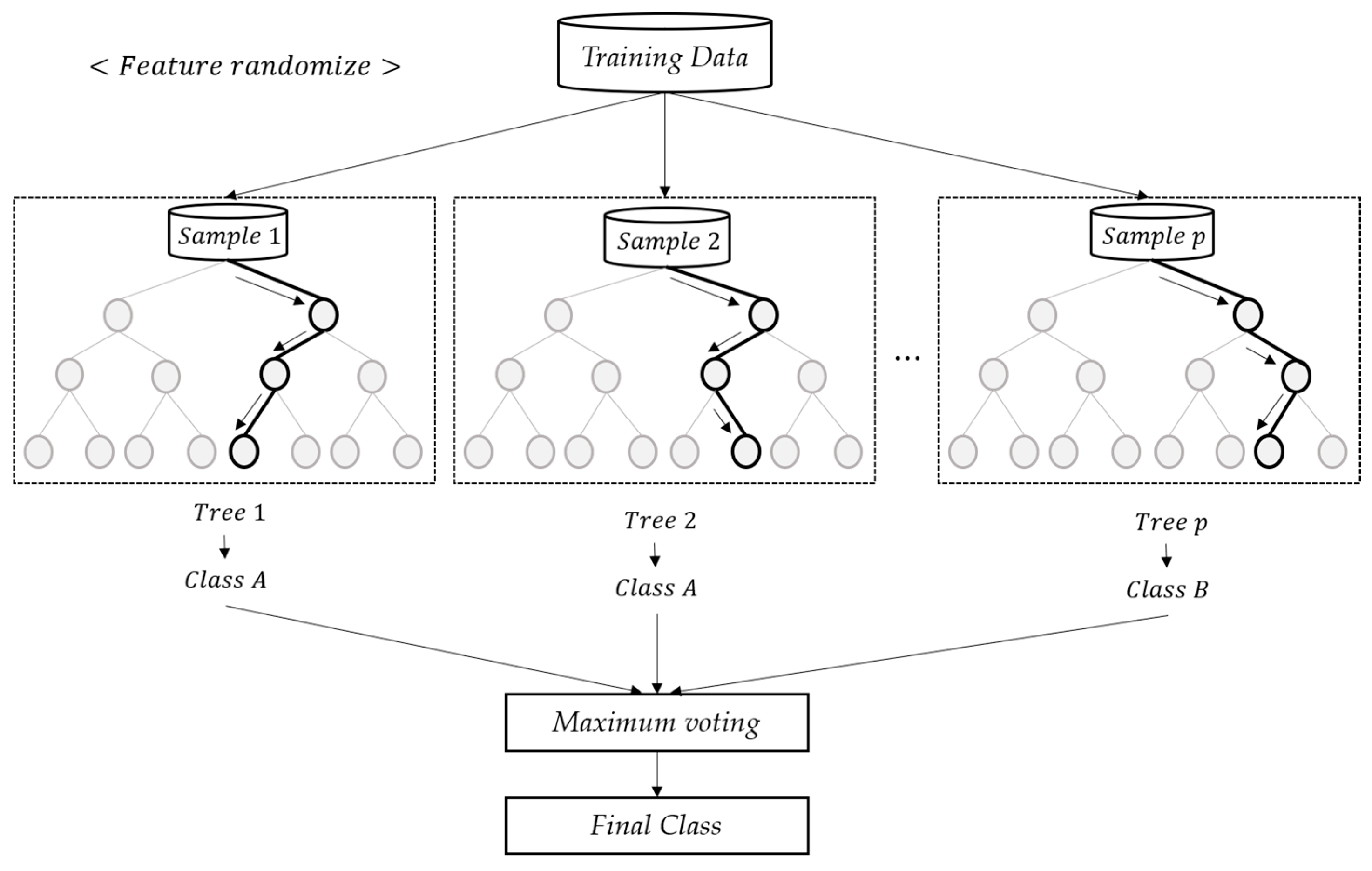
2.1.3. Random Forest
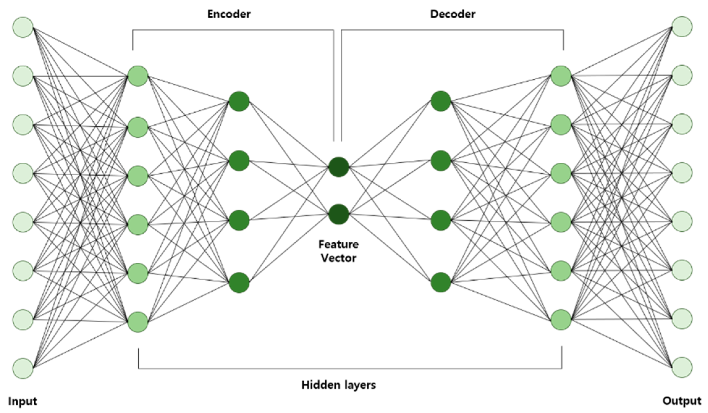
2.1.4. Autoencoder
- AE is trained using input data and then the learned data are acquired.
- Learned data from the previous layer are used continuously as input for the next layer until the training is completed.
- Once all the hidden layers are trained, the backpropagation algorithm is used to minimize the cost function and the weights are updated with the training set to achieve fine-tuning.
2.1.5. Classification Performance
Sensitivity = TP/(TP + FN)
Specificity = TN/(TN + FP)
Precision = TP/(TP + FP)
F1-Measure = 2× (Sensitivity × Precision)/(Sensitivity + Precision)
2.2. Materials
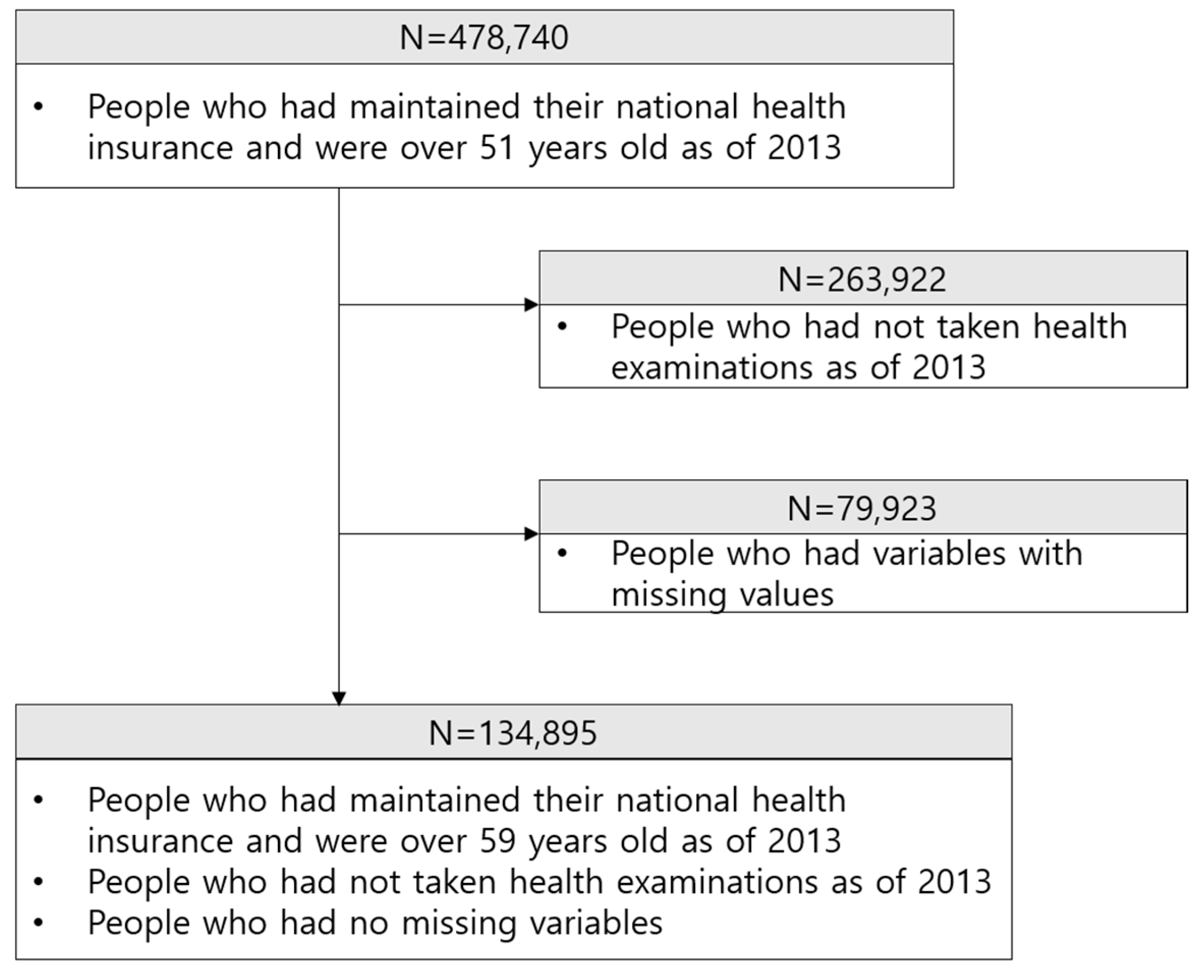
2.2.1. Dataset
2.2.2. Description of Variable
2.2.3. Stages of CKD
2.2.4. The Property and Treatment of Highly Imbalanced Data
2.2.5. Preprocessing
3. Results and Discussion
3.1. Baseline Characteristic of Variables
3.2. Results
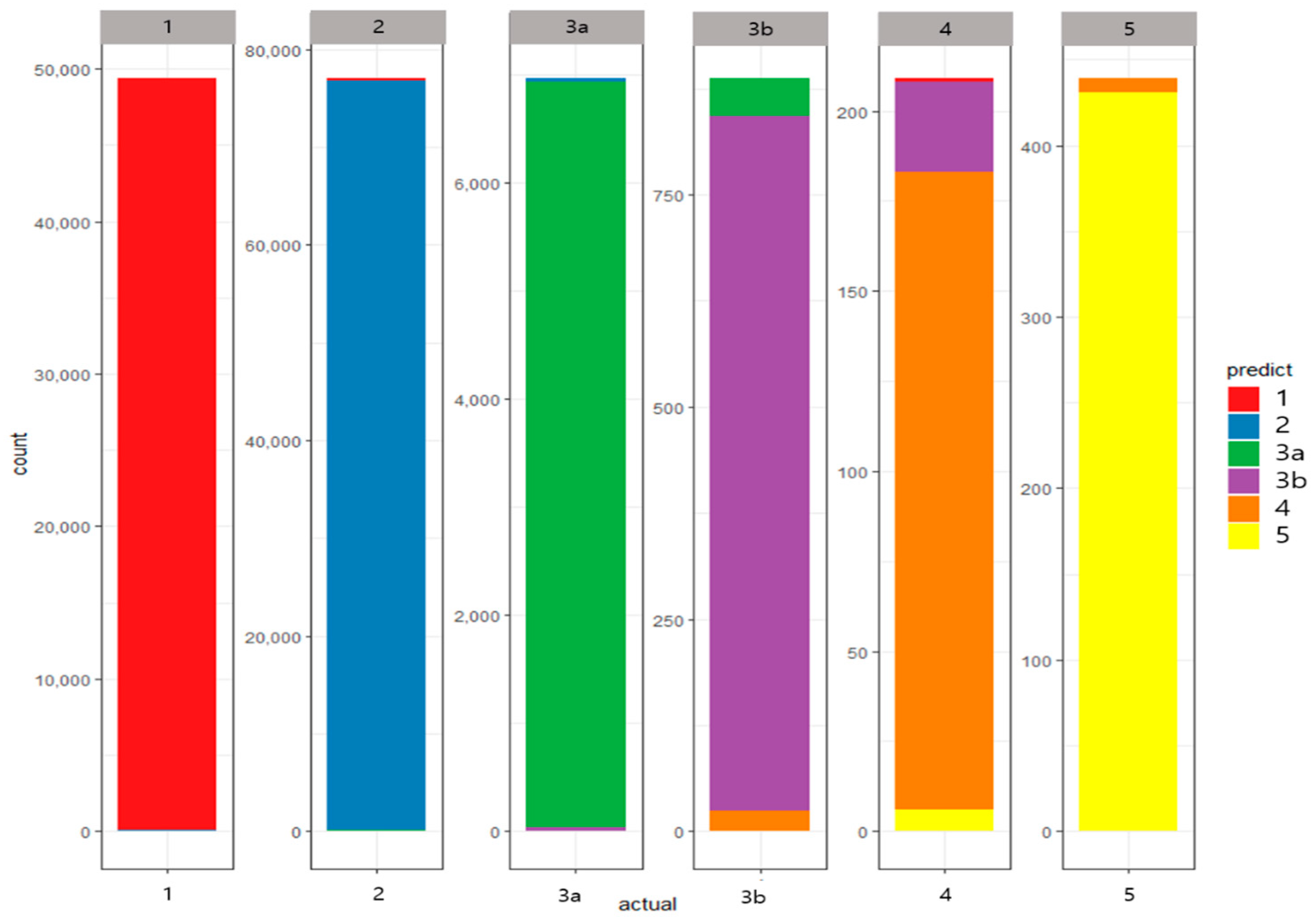
- Stage 1 patients: sensitivity 99.76%, specificity 99.79%, precision 99.64%, and F1-Measure 99.70%
- Stage 2 patients: sensitivity 99.65%, specificity 99.73%, precision 99.80%, and F1-Measure 99.72%
- Stage 3A patients: sensitivity 99.05%, specificity 99.89%, precision 99.97%, and F1-Measure 98.51%
- Stage 3B patients: sensitivity 92.23%, specificity 99.96%, precision 93.77%, and F1-Measure 92.96%
- Stage 4 patients: sensitivity 84.62%, specificity 99.98%, precision 85.94%, and F1-Measure 84.66%
- Stage 5 patients: sensitivity 98.18%, specificity 99.99%, precision 98.21%, and F1-Measure 98.18%
3.3. Discussion
4. Conclusions
Author Contributions
Funding
Acknowledgments
Conflicts of Interest
References
- Stevens, P.E.; Levin, A. Evaluation and management of chronic kidney disease: Synopsis of the kidney disease: Improving global outcomes 2012 clinical practice guideline. Ann. Intern. Med. 2013, 158, 825–830. [Google Scholar] [CrossRef] [PubMed] [Green Version]
- Kidney Disease Improving Global Outcomes. KDIGO 2012 Clinical Practice Guideline for the Evaluation and Management of Chronic Kidney Disease. Kidney Int. 2013, 3, 5–14. [Google Scholar]
- Hill, N.R.; Fatoba, S.T.; Oke, J.L.; Hirst, J.A.; O’Callaghan, C.A.; Lasserson, D.S.; Hobbs, F.D.R. Global Prevalence of Chronic Kidney Disease-A Systematic Review and Meta-Analysis. PLoS ONE 2016, 11, e0158765. [Google Scholar] [CrossRef]
- Velde, M.; Matsushita, K.; Coresh, J.; Astor, B.C.; Woodward, M.; Kevey, A.S.; Jong, P.E.; Gransevoort, R.T. Lower estimated glomerular filtration rate and higher albuminuria are associated with all-cause and cardiovascular mortality. A collaborative meta-analysis of high-risk population cohorts. Kidney Int. 2011, 79, 1341–1352. [Google Scholar] [CrossRef] [Green Version]
- Wen, C.P.; Cheng, T.Y.; Tsai, M.K.; Chang, Y.C.; Chan, H.T.; Tsai, S.P.; Chiang, P.H.; Hsu, C.C.; Sung, P.K.; Hsu, Y.H.; et al. All-cause mortality attributable to chronic kidney disease: A prospective cohort study based on 462 293 adults in Taiwan. Lancet 2008, 371, 2173–2182. [Google Scholar] [CrossRef]
- Yarnoff, B.O.; Hoerger, T.J.; Simpson, S.K.; Leib, A.; Burrows, N.R.; Shrestha, S.S.; Pavkov, M.E. The cost-effectiveness of using chronic kidney disease risk scores to screen for early-stage chronic kidney disease. BMC Nephrol. 2017, 18, 85. [Google Scholar] [CrossRef] [Green Version]
- Mena, L.; Gonzalez, J.A. Symbolic One-Class Learning from Imbalanced Datasets: Application in Medical Diagnosis. Int. J. Artif. Intell. Tools 2009, 18, 273–309. [Google Scholar] [CrossRef]
- Magnin, B.; Mesrob, L.; Kinkingnéhun, S.; Pélégrini-Issac, M.; Colliot, O.; Sarazin, M.; Dubois, B.; Lehéricy, S.; Benali, H. Support vector machine-based classification of Alzheimer’s disease from whole-brain anatomical MRI. Neuroradiology 2009, 51, 73–83. [Google Scholar] [CrossRef]
- Yu, W.; Liu, T.; Valdez, R.; Gwinn, M.; Khoury, M.J. Application of Support Vector Machine Modeling for Prediction of Common Diseases: The Case of Diabetes and Pre-Diabetes. BMC Med. Inform. Decis. Mak. 2010, 10, 16. [Google Scholar] [CrossRef] [Green Version]
- Dessai, I.S.F. Intelligent heart disease prediction system using probabilistic neural network. IJACTE 2013, 2, 2319–2526. [Google Scholar]
- Cao, Y.; Hu, Z.D.; Liu, X.F.; Deng, A.M.; Hu, C.J. An MLP classifier for prediction of HBV-induced liver cirrhosis using routinely available clinical parameters. Dis. Markers 2013, 35, 653–660. [Google Scholar] [CrossRef] [PubMed] [Green Version]
- Rady, E.A.; Anwar, A.S. Prediction of kidney disease stages using data mining algorithms. Inform. Med. Unlocked 2019, 15. [Google Scholar] [CrossRef]
- He, H.; Garcia, E.A. Learning from Imbalanced Data. IEEE Trans. Knowl. Data Eng. 2009, 21, 1263–1284. [Google Scholar]
- Anand, A.; Pugalenthi, G.; Fogel, G.B.; Suganthan, P.N. An approach for classification of highly imbalanced data using weighting and undersampling. Amino Acids 2010, 39, 1385–1391. [Google Scholar] [CrossRef]
- Galar, M.; Fernandez, A.; Barrenechea, E.; Herrera, F. EUSBoost: Enhancing ensembles for highly imbalanced data-sets by evolutionary undersampling. Pattern Recognit. 2013, 46, 3460–3471. [Google Scholar] [CrossRef]
- García, V.; Sánchez, J.S.; Mollineda, R.A. On the effectiveness of preprocessing methods when dealing with different levels of class imbalance. Knowl.-Based Syst. 2012, 25, 13–21. [Google Scholar] [CrossRef]
- Ng, W.W.Y.; Zeng, G.; Zhang, J.; Yeung, D.S.; Pedrycz, W. Dual autoencoders features for imbalance classification problem. Pattern Recognit. 2016, 60, 875–889. [Google Scholar] [CrossRef]
- Wasikowski, M.; Chen, X.-W. Combating the small sample class imbalance problem using feature selection. IEEE Trans. Knowl. Data Eng. 2010, 22, 1388–1400. [Google Scholar] [CrossRef]
- Zhang, C.; Song, J.; Gao, W.; Jiang, J. An Imbalanced Data Classification Algorithm of Improved Autoencoder Neural Network. In Proceedings of the 8th International Conference on Advanced Computational Intelligence, Chiang Mai, Thailand, 14–16 February 2016. [Google Scholar]
- Wan, Z.; Zhang, T.; He, H. Variational Autoencoder Based Synthetic Data Generation for Imbalanced Learning. In Proceedings of the 2017 IEEE Symposium Series on Computational Intelligence, Honolulu, HI, USA, 27 November–1 December 2017. [Google Scholar]
- Shen, C.; Zhang, S.F.; Zhai, J.H.; Luo, D.S.; Chen, J.F. Imbalanced Data Classification Based on Extreme Learning Machine Autoencoder. In Proceedings of the 2018 International Conference on Machine Learning and Cybernetics, Chengdu, China, 15–18 July 2018. [Google Scholar]
- King, G.; Zeng, L. Logistic regression in rare event data. Political Anal. 2001, 9, 137–163. [Google Scholar] [CrossRef] [Green Version]
- Agresti, A. Categorical Data Analysis; WILEY: Hoboken, NJ, USA, 2013. [Google Scholar]
- Ho, T.K. Random Decision Forests. In Proceedings of the 3rd International Conference on Document Analysis and Recognition, Montreal, QC, Canada, 14–16 August 1995; pp. 278–282. [Google Scholar]
- Ho, T.K. The Random Subspace Method for Constructing Decision Forests. IEEE Trans. Pattern Anal. Mach. Intell. 1998, 20, 832–844. [Google Scholar]
- Liu, G.; Bao, H.; Han, B. A Stacked Autoencoder-Based Deep Neural Network for Achieving Gearbox Fault Diagnosis. Math. Probl. Eng. 2018, 2018. Available online: https://www.hindawi.com/journals/mpe/2018/5105709/ (accessed on 18 June 2020). [CrossRef] [Green Version]


| Variable | Type | Class | Description | |
|---|---|---|---|---|
| CKD_eGFR | Categorical | Target | eGFR using MDRD | 1, 2, 3A, 3B, 4, 5 |
| INCOME_DECILES | Categorical | Predictor | Income deciles | 0, 1, 2, …, 10 |
| DISABILITY | Categorical | Predictor | Type of disability | 0: Not disabled (Normal) 1: Mild 2: Severe |
| SEX | Categorical | Predictor | Gender | 1: Male 2: Female |
| SMOKING_STATUS | Categorical | Predictor | Smoking status | 1: No 2: Past 3: Current |
| AGE | Numerical | Predictor | Age | - |
| BLDS | Numerical | Predictor | Fasting blood sugar | mg/dL |
| BMI | Numerical | Predictor | Body mass index | Weight(kg)/(Height × Height(m2)) |
| BP_HIGH | Numerical | Predictor | Systolic pressure | mmHg |
| BP_LWST | Numerical | Predictor | Diastolic pressure | mmHg |
| CREATININE | Numerical | Predictor | Serum Creatinine | mg/dL |
| GAMMA_GTP | Numerical | Predictor | Gamma Glutamyl Transpeptidase (GTP) | U/L |
| HDL_CHOLE | Numerical | Predictor | High Density Lipoprotein (HDL) Cholesterol | mg/dL |
| HMG | Numerical | Predictor | Hemoglobin | g/dL |
| LDL_CHOLE | Numerical | Predictor | Low Density Lipoprotein (LDL) Cholesterol | mg/dL |
| SGOT_AST | Numerical | Predictor | AST (Aspartate Amino-Transferase) | U/L |
| SGPT_ALT | Numerical | Predictor | ALT (Alanine Amino-Transferase) | U/L |
| TOT_CHOLE | Numerical | Predictor | Total Cholesterol | mg/dL |
| TRIGLYCERIDE | Numerical | Predictor | Triglycerides | mg/dL |
| WAIST | Numerical | Predictor | Waist measure | cm |
| Stage | GFR | Description |
| 1 | ≥90 | Normal or high |
| 2 | 60~89 | Mildly decreased |
| 3A | 45~59 | Mildly to moderately decreased |
| 3B | 30~44 | Moderately to severely decreased |
| 4 | 15~29 | Severely decreased |
| 5 | <15 | Kidney Failure |
| Variable | GFR-MDRD (Mean ± SD or N (%)) | |||||||
|---|---|---|---|---|---|---|---|---|
| Total | ≥90 (1) | 60~89 (2) | 45~69 (3a) | 30~44 (3b) | 15~29 (4) | <15 (5) | ||
| N (%) | 134,895 | 49,378 (36.6) | 77,018 (57.09) | 6964 (5.16) | 887 (0.66) | 209 (0.15) | 439 (0.33) | |
| INCOME_DECILES | 0 | 651 | 9447 (33.36) | 17,157 (60.59) | 1382 (4.88) | 188 (0.66) | 36 (0.13) | 105 (0.37) |
| 1 | 9714 | 227 (34.87) | 349 (53.61) | 55 (8.45) | 8 (1.23) | 4 (0.61) | 8 (1.23) | |
| 2 | 8331 | 3321 (34.19) | 5622 (57.88) | 649 (6.68) | 78 (0.8) | 19 (0.2) | 25 (0.26) | |
| 3 | 9405 | 3151 (37.82) | 4627 (55.54) | 463 (5.56) | 50 (0.6) | 19 (0.23) | 21 (0.25) | |
| 4 | 8643 | 3715 (39.5) | 5095 (54.17) | 499 (5.31) | 63 (0.67) | 15 (0.16) | 18 (0.19) | |
| 5 | 9793 | 3374 (39.04) | 4749 (54.95) | 427 (4.94) | 54 (0.62) | 9 (0.1) | 30 (0.35) | |
| 6 | 11,120 | 3877 (39.59) | 5338 (54.51) | 480 (4.9) | 52 (0.53) | 11 (0.11) | 35 (0.36) | |
| 7 | 12,848 | 4465 (40.15) | 5970 (53.69) | 548 (4.93) | 64 (0.58) | 20 (0.18) | 53 (0.48) | |
| 8 | 15,444 | 5054 (39.34) | 7082 (55.12) | 597 (4.65) | 74 (0.58) | 11 (0.09) | 30 (0.23) | |
| 9 | 20,631 | 5720 (37.04) | 8745 (56.62) | 815 (5.28) | 105 (0.68) | 23 (0.15) | 36 (0.23) | |
| 10 | 28,315 | 7027 (34.06) | 12,284 (59.54) | 1049 (5.08) | 151 (0.73) | 42 (0.2) | 78 (0.38) | |
| DISABLED_TYPE | Normal | 134,067 | 49,146 (36.66) | 76,552 (57.1) | 6874 (5.13) | 861 (0.64) | 204 (0.15) | 430 (0.32) |
| Mild | 606 | 173 (28.55) | 350 (57.76) | 61 (10.07) | 19 (3.14) | 3 (0.5) | 0 (0) | |
| Severe | 222 | 59 (26.58) | 116 (52.25) | 29 (13.06) | 7 (3.15) | 2 (0.9) | 9 (4.05) | |
| SEX | Male | 77,118 | 28,095 (36.43) | 44,944 (58.28) | 3229 (4.19) | 488 (0.63) | 125 (0.16) | 237 (0.31) |
| Female | 57,777 | 21,283 (36.84) | 32,074 (55.51) | 3735 (6.46) | 399 (0.69) | 84 (0.15) | 202 (0.35) | |
| SMOKING_STATUS | No | 82,346 | 29,766 (36.15) | 46,724 (56.74) | 4857 (5.9) | 585 (0.71) | 133 (0.16) | 281 (0.34) |
| Past | 30,885 | 10,538 (34.12) | 18,580 (60.16) | 1393 (4.51) | 214 (0.69) | 54 (0.17) | 106 (0.34) | |
| Current | 21,664 | 9074 (41.89) | 11,714 (54.07) | 714 (3.3) | 88 (0.41) | 22 (0.1) | 52 (0.24) | |
| AGE | 60.87 ± 8 | 58.75 ± 6.67 | 61.49 ± 8.2 | 67.5 ± 8.29 | 70.7 ± 9.03 | 69.06 ± 8.91 | 62.36 ± 7.94 | |
| BLDS | 102.53 ± 24.44 | 101.81 ± 24.19 | 102.45 ± 23.69 | 106.5 ± 29.13 | 113.19 ± 39.61 | 114.91 ± 47.65 | 106.52 ± 30.7 | |
| BMI | 24.01 ± 2.92 | 23.77 ± 2.93 | 24.11 ± 2.88 | 24.56 ± 3.01 | 24.66 ± 3.17 | 24.17 ± 3.53 | 24.09 ± 2.92 | |
| BP_HIGH | 124.6 ± 14.51 | 124.11 ± 14.41 | 124.59 ± 14.4 | 127.16 ± 15.43 | 128.45 ± 16.51 | 131.88 ± 18.23 | 130.11 ± 16.64 | |
| BP_LWST | 76.89 ± 9.51 | 76.86 ± 9.57 | 76.9 ± 9.43 | 77.01 ± 9.83 | 75.95 ± 10 | 77.03 ± 10.72 | 77.79 ± 9.93 | |
| CREATININE | 0.92 ± 0.55 | 0.74 ± 0.14 | 0.96 ± 0.15 | 1.21 ± 0.18 | 1.65 ± 0.27 | 2.58 ± 0.56 | 8.2 ± 5.17 | |
| GAMMA_GTP | 36.46 ± 49.03 | 37.91 ± 55.22 | 35.79 ± 45.42 | 33.84 ± 40.86 | 37.98 ± 53.29 | 31.73 ± 29.1 | 31.32 ± 29.53 | |
| HDL_CHOLE | 53.37 ± 15.84 | 54.49 ± 15.75 | 52.96 ± 15.82 | 50.89 ± 16.4 | 47.05 ± 12.89 | 47.33 ± 14 | 53.06 ± 14.39 | |
| HMG | 14.08 ± 1.44 | 14.08 ± 1.38 | 14.14 ± 1.43 | 13.55 ± 1.55 | 12.68 ± 1.69 | 11.49 ± 1.72 | 13.21 ± 1.97 | |
| LDL_CHOLE | 117.67 ± 34.89 | 116.19 ± 34.99 | 118.98 ± 34.5 | 116.08 ± 37.08 | 105.83 ± 37.7 | 101.01 ± 33.05 | 111.74 ± 36.33 | |
| SGOT_AST | 26.39 ± 15.74 | 26.34 ± 15.07 | 26.45 ± 16.39 | 26.58 ± 13.09 | 25.6 ± 16.03 | 23.33 ± 11 | 23.05 ± 8.9 | |
| SGPT_ALT | 24.55 ± 17.84 | 24.74 ± 18.19 | 24.59 ± 17.81 | 23.42 ± 15.96 | 21.7 ± 18.24 | 18.85 ± 12.85 | 20.7 ± 10.24 | |
| TOT_CHOLE | 197.16 ± 37.23 | 196.16 ± 36.48 | 198.24 ± 37.19 | 195.01 ± 40.87 | 184.52 ± 42.64 | 176.32 ± 39.99 | 190.56 ± 40.51 | |
| TRIGLYCERIDE | 133.14 ± 81.97 | 130.33 ± 83.11 | 133.9 ± 81.16 | 141.36 ± 79.96 | 160.87 ± 98.44 | 136.99 ± 61.22 | 128.22 ± 76.73 | |
| WAIST | 82.04 ± 8.21 | 81.26 ± 8.15 | 82.33 ± 8.17 | 83.81 ± 8.38 | 85.45 ± 8.52 | 84.33 ± 9.68 | 82.39 ± 8.37 | |
| Method | Class | Accuracy (S.D.) | Sensitivity (S.D.) | Specificity (S.D.) | Precision (S.D.) | F1-Measure (S.D.) |
|---|---|---|---|---|---|---|
| Multinomial LR | 1 | 0.8244 (0.0153) | 0.9217 (0.0191) | 0.8764 (0.0240) | 0.8125 (0.0306) | 0.8633 (0.0205) |
| 2 | 0.8482 (0.0176) | 0.8025 (0.0157) | 0.8510 (0.0122) | 0.8496 (0.0142) | ||
| 3A | 0.0113 (0.0094) | 0.9968 (0.0024) | 0.1426 (0.0771) | - | ||
| 3B | 0.0091 (0.0139) | 0.9969 (0.0034) | 0.0000 (0.0000) | - | ||
| 4 | 0.0195 (0.0345) | 0.9977 (0.0028) | 0.0105 (0.0184) | - | ||
| 5 | 0.6249 (0.3307) | 0.9960 (0.0029) | 0.3814 (0.1947) | - | ||
| Ordinal LR | 1 | 0.9682 (0.0010) | 0.9797 (0.0019) | 0.9982 (0.0011) | 0.9796 (0.0018) | 0.9797 (0.0013) |
| 2 | 0.9746 (0.0014) | 0.9651 (0.0022) | 0.9738 (0.0016) | 0.9742 (0.0010) | ||
| 3A | 0.8363 (0.0101) | 0.9916 (0.0006) | 0.8440 (0.0099) | 0.8401 (0.0077) | ||
| 3B | 0.8265 (0.0345) | 0.9989 (0.0003) | 0.8332 (0.0381) | 0.8293 (0.0297) | ||
| 4 | 0.8319 (0.1167) | 0.9997 (0.0001) | 0.8314 (0.0555) | 0.8269 (0.0655) | ||
| 5 | 0.9818 (0.0209) | 0.9999 (0.0001) | 0.9802 (0.0240) | 0.9807 (0.0118) | ||
| RF | 1 | 0.9948 (0.0015) | 0.9998 (0.0002) | 0.9997 (0.0002) | 0.9995 (0.0004) | 0.9997 (0.0003) |
| 2 | 0.9996 (0.0003) | 0.9969 (0.0013) | 0.9976 (0.0010) | 0.9986 (0.0006) | ||
| 3A | 0.9792 (0.0084) | 0.9977 (0.0008) | 0.9594 (0.0136) | 0.9692 (0.0104) | ||
| 3B | 0.7578 (0.0799) | 0.9989 (0.0003) | 0.8156 (0.0475) | 0.7848 (0.0618) | ||
| 4 | 0.2771 (0.1445) | 0.9998 (0.0002) | 0.6170 (0.2700) | - | ||
| 5 | 0.6585 (0.1342) | 0.9998 (0.0001) | 0.9270 (0.0549) | 0.7629 (0.1010) | ||
| AE | 1 | 0.9958 (0.0005) | 0.9976 (0.0010) | 0.9979 (0.0005) | 0.9964 (0.0009) | 0.9970 (0.0005) |
| 2 | 0.9965 (0.0008) | 0.9973 (0.0009) | 0.9980 (0.0007) | 0.9972 (0.0005) | ||
| 3A | 0.9905 (0.0039) | 0.9989 (0.0004) | 0.9797 (0.0063) | 0.9851 (0.0032) | ||
| 3B | 0.9223 (0.0281) | 0.9996 (0.0001) | 0.9377 (0.0257) | 0.9296 (0.0183) | ||
| 4 | 0.8462 (0.1181) | 0.9998 (0.0002) | 0.8594 (0.0762) | 0.8466 (0.0658) | ||
| 5 | 0.9818 (0.0179) | 0.9999 (0.0001) | 0.9821 (0.0231) | 0.9818 (0.0178) |
| Method | Macro Sensitivity | Micro Sensitivity | Macro Precision | Micro Precision | Macro F1-Measure | Micro F1-Measure |
|---|---|---|---|---|---|---|
| Multinomial LR | 0.4058 | 0.8244 | 0.3663 | 0.7919 | 0.8565 | - |
| Ordinal LR | 0.9051 | 0.9682 | 0.9070 | 0.9681 | 0.9052 | 0.9681 |
| RF | 0.7787 | 0.9948 | 0.8860 | 0.9943 | 0.9030 | - |
| AE | 0.9558 | 0.9958 | 0.9589 | 0.9958 | 0.9562 | 0.9958 |
© 2020 by the authors. Licensee MDPI, Basel, Switzerland. This article is an open access article distributed under the terms and conditions of the Creative Commons Attribution (CC BY) license (http://creativecommons.org/licenses/by/4.0/).
Share and Cite
Jeong, B.; Cho, H.; Kim, J.; Kwon, S.K.; Hong, S.; Lee, C.; Kim, T.; Park, M.S.; Hong, S.; Heo, T.-Y. Comparison between Statistical Models and Machine Learning Methods on Classification for Highly Imbalanced Multiclass Kidney Data. Diagnostics 2020, 10, 415. https://doi.org/10.3390/diagnostics10060415
Jeong B, Cho H, Kim J, Kwon SK, Hong S, Lee C, Kim T, Park MS, Hong S, Heo T-Y. Comparison between Statistical Models and Machine Learning Methods on Classification for Highly Imbalanced Multiclass Kidney Data. Diagnostics. 2020; 10(6):415. https://doi.org/10.3390/diagnostics10060415
Chicago/Turabian StyleJeong, Bomi, Hyunjeong Cho, Jieun Kim, Soon Kil Kwon, SeungWoo Hong, ChangSik Lee, TaeYeon Kim, Man Sik Park, Seoksu Hong, and Tae-Young Heo. 2020. "Comparison between Statistical Models and Machine Learning Methods on Classification for Highly Imbalanced Multiclass Kidney Data" Diagnostics 10, no. 6: 415. https://doi.org/10.3390/diagnostics10060415