Article

A Performance-Driven MPC Algorithm for Underactuated Bridge Cranes †

1
Department of Control Science and Engineering, Tongji University, Shanghai 201804, China
2
Shanghai Institute of Intelligent Science and Technology, Tongji University, Shanghai 200092, China
3
School of Electrical and Electronic Engineering, Shanghai Institute of Technology, Shanghai 201418, China
4
Department of Electrical and Computer Engineering, New Jersey Institute of Technology, Newark, NJ 07102, USA
5
Department of Electrical and Computer Engineering, Center of Research Excellence in Renewable Energy and Power Systems, King Abdulaziz University, Jeddah 21481, Saudi Arabia
*
Authors to whom correspondence should be addressed.
This paper is an extended version of our conference paper: Bao, H.Q.; An, J.; Zhou, M.C.; Kang, Q. “A Data-driven MPC Algorithm for Bridge Cranes” 2020 International Conference on Advanced Mechatronic Systems (ICAMechS), 20341486 (10–13 December 2020).
Machines 2021, 9(8), 177; https://doi.org/10.3390/machines9080177
Submission received: 7 July 2021 / Revised: 3 August 2021 / Accepted: 9 August 2021 / Published: 20 August 2021
(This article belongs to the Special Issue Design and Control of Advanced Mechatronics Systems)

Abstract

:
A crane system often works in a complex environment. It is difficult to model or learn its true dynamics by traditional system identification approaches. If a dynamics model is created by minimizing its prediction error, its use tends to introduce inaccuracies and thus lead to suboptimal performance. Is it possible to learn the dynamics model of a crane that can achieve the best performance, instead of learning its true dynamics? This work answers the question by presenting a performance-driven model predictive control (P-MPC) algorithm for a two-dimensional underactuated bridge crane. In the proposed dual-layer control architecture, an inner-loop controller uses a proportional–integral–derivative controller to achieve anti-sway rapidly. An outer-loop controller uses MPC to ensure accurate trolley positioning under control constraints. Compared with classical MPC, this work proposes a data-driven method for plant modeling and controller parameter updating. By considering the control target at the learning stage, the method can avoid adjusting the controller to deal with uncertainty. We use Bayesian optimization in an active learning framework where a locally linear dynamics model is learned with the intent of maximizing control performance and then used in conjunction with optimal control schemes to efficiently design a controller for a given task. The model is updated directly based on the performance observed in experiments on the physical system in an iterative manner till a desired performance is achieved. The controller parameters and prediction models of the best closed-loop performance can be found through continuous experiments and iterative optimization. Simulation and experiment results show that we can explicitly find the dynamics model that produces the best performance for an actual system, and the method can quickly suppress swing and realize accurate trolley positioning. The results verified its effectiveness, feasibility, and superior performance on comparing it with state-of-the-art methods.

1. Introduction

A mechanical system with fewer drivers than the degree of freedom is called an underactuated one [1]. The reduction of drivers can make them light and flexible. Therefore, it is widely used in industry [2]. Underactuated systems are often divided into two categories. The first contains underactuated mechanical systems with restricted movement [3,4], including a mobile robot, shuttle, underwater vehicle, and underwater underactuated robot. They cannot move sideways, or they must follow a fixed trajectory. The second covers underactuated mechanical arm type systems, mainly including different types of cranes (such as bridge, cantilever, and tower cranes), the inverted pendulum system, the ball and beam system, the translational oscillator with rotating actuator, and the pendulum robot. The state of this type of system is analogous to a shift from a connecting rod or a rotation. The reduction of the number of drivers can increase coupling among the system components and the complexity of the system, making its controller design more difficult. In recent decades, the underactuated mechanical system’s control problem has been a long-term challenging problem in control engineering. Moreover, under particular circumstances, a fully actuated system may become an underactuated system when any actuator partially fails, or a running trajectory is fixed. Therefore, the in-depth study of underactuated mechanical systems is of essential theoretical and practical significance.
As a typical underactuated mechanical arm system, a bridge crane is an essential means of cargo transportation. It is widely used in construction sites, ports, production workshops, warehouses, and other industrial fields [5]. Its main control objectives can be summarized as accurately transporting goods to a target location and suppressing load swing as much as possible. The payload’s swing angle must be small enough to avoid accidents in the process of transportation. Suppose that a bridge crane’s swing is too large then in that case, it affects its operational safety and production efficiency. Due to the lack of several actuators, its payload swing angle is underactuated, making such an angle difficult to control. How to suppress payload swing and ensure a trolley’s accurate positioning is an important yet challenging issue to be addressed. The coupling or accompanying nonholonomic constraints on a crane system state increases the difficulty in designing an underactuated crane control system.
In recent years, researchers have made some noticeable progress in controlling bridge cranes. An in-depth analysis of their dynamics has been conducted and a reasonable motion trajectory for their trolley while considering the load swing angle is planned [6,7,8]. Ouyang et al. proposed an s-shaped motion trajectory generation method that could realize anti-sway [6]. Jaafar et al. proposed a feedforward command shaping method of anti-sway for a bridge crane system [9], which requires fewer sensors than some existing methods. These methods [6,7,8,9] are all open-loop control-based ones and fail to deal with external disturbance. Some closed-loop feedback control methods have been proposed to deal with external disturbance to such a system [10]. The common method is to use proportional–integral–derivative (PID) controllers [11]. Some control algorithms based on state observers are proposed to handle partially unmeasurable states [12,13]. To reveal the effects of unknown disturbances on cranes, Zhang et al. proposed a finite-time trajectory tracking control method based on a state observer [13]. Some complex control methods have been proposed, e.g., passivity-based control schemes in [14,15] and a Lyapunov-based controller in [16]. However, such types of controllers have some inherent defects, e.g., difficult controller design and a narrow scope of application. Some robust controllers have also been proposed to control cranes, such as sliding mode control (SMC) methods [17,18,19,20,21,22,23,24,25]. The work [19] proposed an integral-barrier Lyapunov function (IBLF)-based control method to suppress the undesirable vibrations of the flexible crane system with a boundary output constraint. However, it needs precise partial-ordinary differential equations. Besides, there are some crane system control schemes combined with artificial intelligence, such as fuzzy logic-based [26,27] and neural network-based control [28,29]. These methods draw on human experience to help improve the control performance of a crane.
Most of the methods mentioned above can implement anti-swing. However, they fail to guarantee that such swing is always within its allowable range [30]. Due to the limited power of the crane’s actuator, the large control input tends to cause actuator saturation, thereby reducing control performance and even causing safety problems.
Model predictive control (MPC) can predict the state of a system and handle various constraints. It has been applied to the control problem of bridge cranes [30,31,32,33,34,35]. For example, to deal with constraints, Chen et al. proposed a novel MPC algorithm for 2-D overhead cranes [30], which could deal with actuator saturation. By combining multivariable MPC with particle swarm optimizer (PSO), Smoczek et al. proposed a novel anti-sway method [31]. The methods [30,31] are based on an accurate linearized model. Their application is limited due to model error between the linearized models and their modeled crane systems. Meanwhile, an MPC algorithm requires a high-precision model to achieve superior closed-loop performance.
In adaptive control, model parameters are generally updated to obtain a good prediction model but not necessarily to maximize control performance. Aiming at finding the best predictive model and parameters of a controller from experimental data, we proposed a control method based on performance-driven MPC, which directly considers the crane’s control target at a learning stage. This method requires us to continuously conduct experiments and collect closed-loop data. Although this work is for a small-scale physical crane (e.g., 1:10 size crane) instead of an actual large-scale crane, we can obtain sufficient closed-loop data for a large-scale crane and synthesize a controller by the proposed method. Through continuous iteration and optimization of parameters, the controller for the best performance can be learned and then applied. The performance-driven MPC algorithm framework is shown in Figure 1. It mainly includes three modules: a closed-loop experimental module, a closed-loop control module, and a Bayes-based controller parameter optimization and model learning module [36]. Following [37], we designed a dual-layer control architecture. An inner controller aims to quickly suppress the swing angle, while an outer one can handle control constraints and state ones. The merits of this paper can be summarized as follows.
(1) This work proposes a conversion method to construct a new state augmented system for solving the problem where classical MPC fails to deal with underactuated systems [31,38]. Although a bridge crane’s structure is different from other types of underactuated systems, the dual-layer control architecture in this article can also be applied to other underactuated systems.
(2) Compared with classical MPC algorithms, which require a precise linearization model of a plant to achieve high closed-loop performance, this work proposes a method that does not need specific knowledge of system dynamics characteristics. Using the experimental data for parameter tuning, we can synthesize a controller of excellent performance to achieve fast and accurate trolley positioning and anti-swing control objectives. From the application point of view, the control method is based on data, thereby making it highly applicable to various industrial systems.
The rest of this article is made up as follows. Section 2 briefly introduces the classic MPC and Bayesian optimization. Section 3 introduces a controller’s design, including the parameterization method of each layer of the controller. Section 4 introduces the method of optimizing the parameters based on the data combined with Bayes optimization. Section 5 presents simulation, experimental and comparison results. Section 6 concerns the conclusion.

2. Classic MPC and Bayesian Optimization for a Bridge Crane

This section briefly reviews the methods of classic MPC and Bayesian optimization.

2.1. Classic MPC for Bridge Crane

MPC has gained significant success in recent decades and has become an important control method for handling system constraints [31] as well as a common approach for crane anti-sway. A discrete crane’s dynamics can be described as follows:
x ( k + 1 ) = f ( x ( k ) , u ( k ) , k , w ( k ) )
where u ( k ) n u , x ( k ) n x   and w ( k ) n w are a crane’s input, state, and noise sampled at time k, respectively. nu, nx, and nw are the number for input, state, and noise, respectively.
Classical MPC schemes do not consider any uncertainty for a prediction model. They rely on feedback and the next sampling result to resolve the following problem to compensate for the uncertainty of feedback:
J * = min imize U l f ( x N | k , u N | k , k + N ) + i = 0 N 1 l ( x i | k , u i | k , k + i )
s . t . x i + 1 | k = f ( x i | k , u i | k , k + i ) U = [ u 0 | k , , u N | k ] U j ( j = 1 , , n c u ) X = [ x 0 | k , , x N | k ] X j ( j = 1 , , n c x ) x N | k X f x 0 | k = x ( k )
where U is a control vector. X is a state vector, and l ( x i | k , u i | k , k + i ) is a cost function at time k. ncu and ncx are the number of elements in input sets and state sets. Usually, a cost function is a weighted quadratic cost suitable for tracking tasks. In many MPC formulas, the terminal components lf and Xf are generally imposed for meeting system stability requirements. The MPC control law can be obtained by solving Equation (2), resulting in
u * ( x ( k ) , k ) = u 0 | k *
where u 0 | k *   is the first element of the computes optimal control sequence   U * applied to the crane at time step k.

2.2. Bayesian Optimization for a Bridge Crane

Bayesian optimization is a standard method for training models in machine learning. The objective function’s minimal value can be found by establishing a substitute function (probability model) via the MPC objective function’s past evaluation results. So, we can use Bayesian optimization to optimize the crane model parameters and controller parameters.
Assume that a hyperparameter vector of the bridge crane is X = (x1, x2, …, xn). Different super parameters lead to different effects. Bayesian optimization assumes that there is a functional relationship between the super parameters and the loss function.
Suppose that there is a function f : x ,   x     X . The optimization problem can be described as:
x * = arg min x X f ( x )
Initializing the data-set D = {(xi, yi), …, (xn, yn)}. We can assume f ~ GP( μ ,   κ ) (GP: Gaussian process, μ : mean, and κ : covariance kernel). The forecast also obeys a normal distribution, i.e.,
p ( y | x , D ) = N ( y | μ ^ , σ ^ 2 ) y = ( y 1 y i ) T μ ^ = k ( x ) T ( K + σ n 2 I ) 1 y σ ^ 2 = κ ( x 1 , x ) k ( x ) T ( K + σ n 2 I ) 1 k ( x ) x i arg max x X S ( X , p ( y | x , D ) )
where σ ^ is a covariance matrix, μ ^ is a mean vector, k is the covariance matrix of test sample input and training sample input. K is the covariance matrix between training sample inputs, respectively.
In the next step, we need to select the parameters X that satisfy (5) based on the calculated hypothetical model, then bring the hyperparameters into the network for training, and finally obtain output yi, and update the data set D = {DU(xi, yi)}.
In this paper, we need to consider the balance between exploration and exploitation, and they are defined as follows:
Exploitation: Based on the data collected in the past, search in the area with higher mean value to optimize the performance index, with a high probability of obtaining better results. Note that with such a search it is easy to fall into the local optimum.
Exploration: Learn more about J ¯ in a larger variance area of parameter space.
The acquisition function can be selected in a variety of ways, such as Expected Improvement (EI) and Probability of Improvement. The EI algorithm can balance between exploration and exploitation [39,40,41,42,43]. Thus, the EI acquisition function used in this paper is introduced here. Assuming f ˇ = min   f , and f ˇ represent the minimum value of f , the utility function is defined as follows:   u ( x ) = max   ( 0 ,   f   ˇ   f ( x ) ) , acquisition function can be defined as:
a E I ( x ) = E [ u ( x ) | x , D ] = f ( f f ) N ( f ; μ ( x ) , k ( x , x ) ) d f = ( f μ ( x ) ) Φ ( f ; μ ( x ) , k ( x , x ) ) + k ( x , x ) N ( f ; μ ( x ) , k ( x , x ) )
The point that makes the α E I value maximal is the best point by calculation.

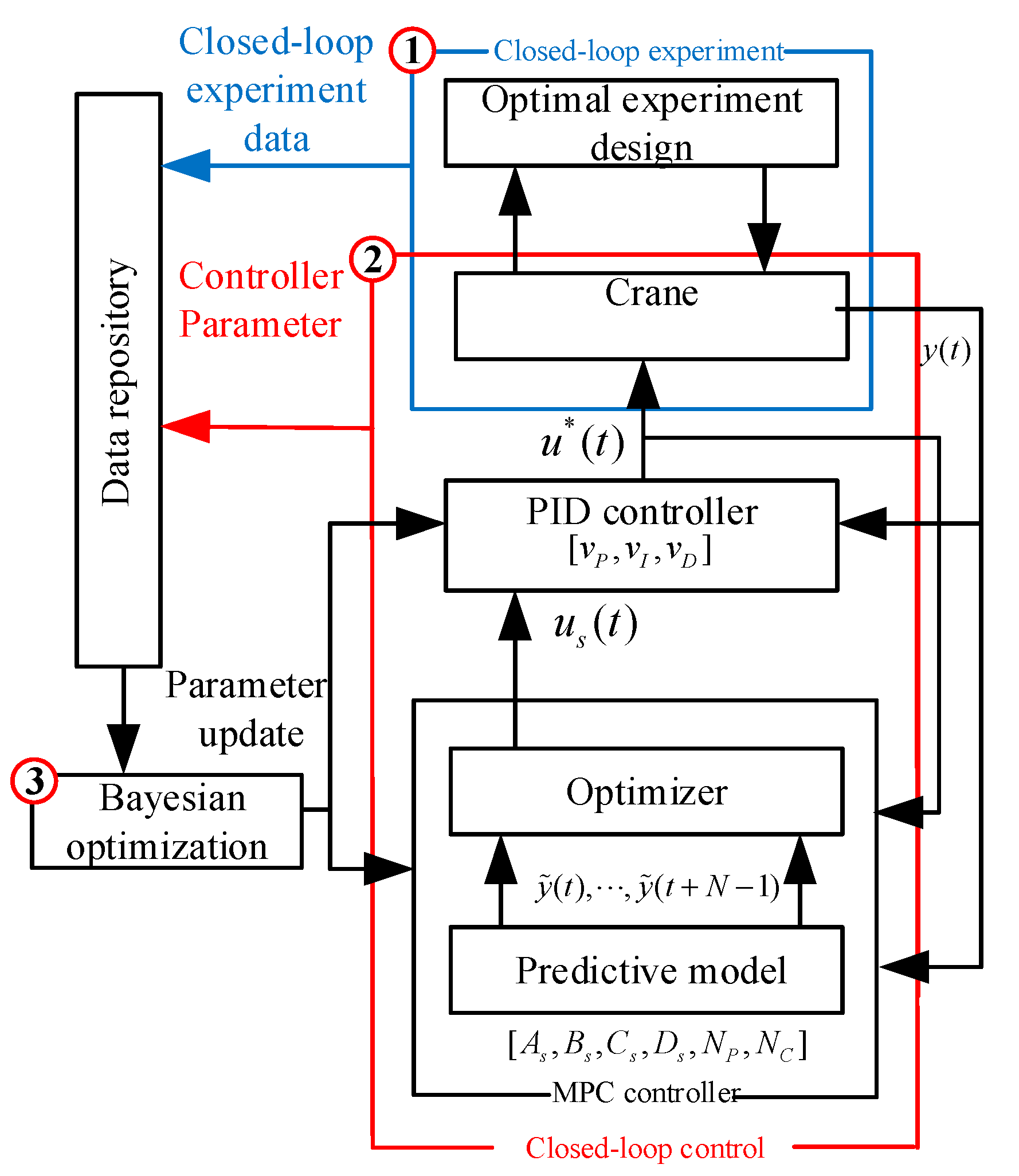
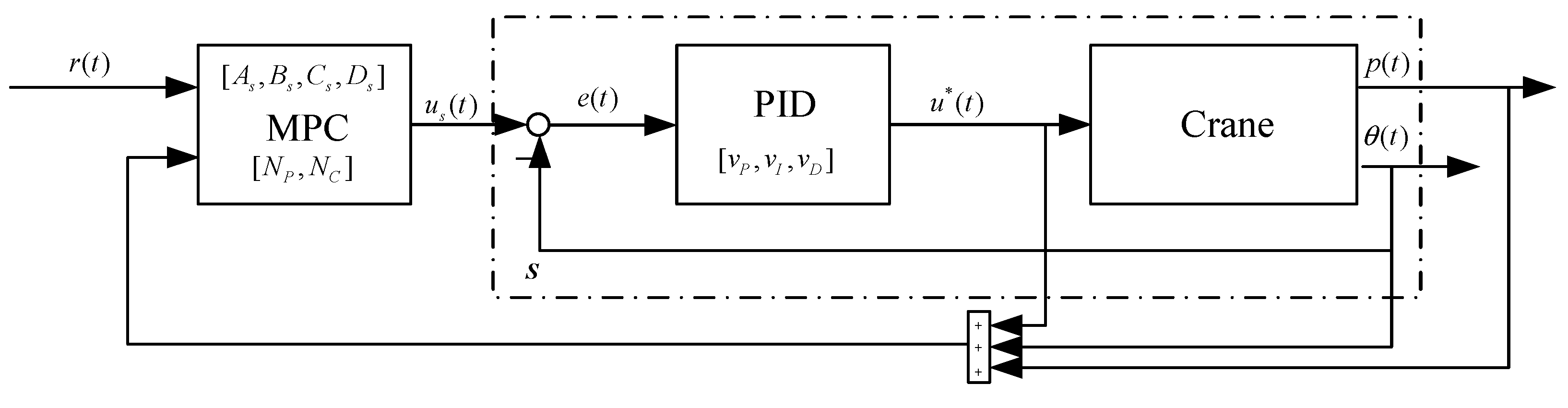
3. Control Architecture

This section presents a dual-layer, multi-rate, tracking control structure, as shown in Figure 2. The inner loop uses a PID controller to achieve rapidly anti-sway at sampling time Ts. To effectively deal with system state constraints and control ones, the outer loop uses MPC to effectively solve an online constraint optimization problem at sampling time TMPC (TMPC = NTs with   N N ). p(t) and θ(t) are the crane’s position and vertical direction angle of the payload, respectively. e(t) is the tracking error of the inner loop system s. r(t) is the reference value. us(t) and u*(t) are the inputs to the inner-loop system s and real input to a crane. A s 2 × 2 , B s 2 × 1 , C s 2 × 2 and D s 2 × 1 are prediction model parameters. ν = [ ν P   ν I   ν D ] is a parameterized vector of a PID controller. NP and NC are MPC parameters.

3.1. Inner PID Controller Parameterization

An inner PID controller is parameterized as a vector ν n ν . The discrete transfer function at the sampling time Ts can be defined as:
G P I D ( z , k ) = υ P + υ I T s 1 z 1 + υ D N d ( z 1 ) z 1 + N d T s
where ν = [ ν P   ν I   ν D ] is a parameterized vector of a PID controller. A filter is added to the differential term ( N d 1 ) for suppressing the high-frequency gain of noise. Nd’s value has little effect on the overall performance. Thus, there is no need to optimize it.

3.2. Outer MPC Controller Parameterization

Consider a one-input and two-output (OITO) plant S as the prediction model of an inner closed-loop system. y s and y = [ p θ ] are the input and output states, respectively. Considering discrete sampling time Ts, we have the following discrete state-space representation:
{ ξ ( t + 1 ) = A s ξ ( t ) + B s y s ( t ) y ¯ = C s ξ ( t ) + D s y s ( t ) y ¯ = [ y ( t ) u * ( t ) ]
where ξ n ξ is the system state that has the transfer functions with the same poles of a crane model. To realize the learning of the parameters of a predictive model, we parameterize A s 2 × 2 , B s 2 × 1 , C s 2 × 2 and D s 2 × 1 into a vector μ n μ .
At time t = nTMPC ( n N ), the outer MPC solves the following optimization problem:
J = min { y s ( t + k | t ) } k = 1 N c , ε Q y k = 1 N p ( y ¯ ( t + k | t ) y r ( t + k | t ) ) 2 + Q u k = 1 N p ( u s * ( t + k | t ) u r ( t + k | t ) ) 2 + Q Δ u k = 1 N p ( u s ( t + k | t ) u s ( t + k 1 | t ) ) 2 + Q ε ε 2
s . t . y ¯ = S ( μ , y s ( t + k | t ) ) , k = 1 , , N p y ¯ λ y ε y ¯ ( t + k | t ) y ¯ ^ λ y ε , k = 1 , , N p u s λ u ε u ( t + k | t ) u ^ s λ u ε , k = 1 , , N p Δ u s λ Δ u ε Δ u s ( t + k | t ) Δ u ^ s λ Δ u ε , k = 1 , , N p u s ( t + N c + k | t ) = u s ( t + N c | t ) , k = 1 , , N p N c
where Δ u s ( t + k   |   t ) , y ¯ ( t + k   |   t ) and u s ( t + N c   |   t ) are the kth control increment, output and input of plant S at time t, respectively. y ¯ ^ = [5, 0.2, 10] and y ¯ = [0, −0.2, −10] are the upper and lower bounds of the output, u ^ s = 10 and u ˇ s = 10 are the upper and lower bounds of input, Δ u ^ s = 1 and Δ u ˇ s = 1 are the upper and lower bounds of the control increment. ur is an input reference, and yr is an output reference. Np is the prediction horizon, and Nc is the control horizon.   Q y ,   Q u ,   Q Δ u and Q ε are the non-negative weights of output, input, control increment, and a relaxation factor, respectively. ε is the corresponding relaxation positive factor. λ y ,   λ u and λ Δ u are the coefficients of the ε . According to the standard MPC design, there is a hard constraint N c N p that needs to be enforced in the parameter learning.
In this paper, we only consider Np and Nc as the tuning parameters, which significantly impact on the closed-loop control performance. We define the overall vector of tuning parameters as a η = [ μ T   N p   N c ] T ( η n μ × × ), n μ is the number of parameters in the controller. We use empirical values instead of learning the parameters by optimization for λ y ,   λ u ,   λ Δ u ,   Q y ,   Q u ,   Q Δ u and Q ε in this paper to reduce the number of parameters to be tuned.

4. P-MPC Parameter Tuning

The designed architecture of a controller and controller parameterization was introduced in the previous section. This section introduces a closed-loop performance function and parameter tuning method based on Bayesian optimization

4.1. Closed-Loop Performance Index

To realize the trolley accurately positioning and the payload anti-swing, the following evaluation function J ¯ is designed for accurately evaluating the performance of a closed-loop control algorithm.
J ¯ ( y T , u T ; η , υ ) = log [ 1 T t = 1 T ( 2 | p ( t ) r p | + 0 . 5 | θ ( t ) r θ | ) ] + log [ 1 T t = 1 T τ ( p ( t ) ) + 1 ]
τ ( p ) = { 20 ( | p | p s e t ) , | p | > p s e t 0 , | p | p s e t
where ( y T , u T ) is the measured signal of output and input at sampling time t = 1, …, T, respectively. T is the duration of the closed-loop simulation. vi and η i are the i-th Bayesian optimization results of v and η . io is the optimal solution index. τ is a penalty function that considers the physical constraints on the positioning of trolley pset. This function will hopefully limit the overshoot of the trolley displacement and prevent the occurrence of safety accidents. The crane’s displacement and swing angle data are obtained through closed-loop simulation experiments.
The closed-loop performance J ¯ is calculated according to (12). The parameter optimization problem of the controller can be described as follows:
min η , υ D J ¯ ( y T , u T ; η , υ )
where D is the set of controller parameter candidates.

4.2. P-MPC Controller Parameter Tuning

The Bayesian optimization algorithm has two steps:
1. Construct a Gaussian process regression model [40] and update its parameters through a sampling dataset D; and
2. Build an extracting function to guide the next sampling step, which is referred to as extraction/collection for short.
A controller parameter tuning problem can be solved by minimizing (14). In this paper, we use a Bayesian optimization (BO) strategy to do so. Similar to the work [37], parameter tuning is summarized in Algorithm 1. Our goal is to update effectively the hyperparameters when new data is observed.
Algorithm 1 P-MPC Controller Parameter Tuning
Input: data-set with controller parameters, input, and output
 1. Initialize data-set with parameters and performance as
           D   { ( ν m , η m ) ,   J ¯ m }
 2. For i = m, …, Nmax − 1 do
  2.1 Train a GP approximating J ¯ according to data set D
  2.2 Design the AC function α ( ν , η   |   D ) according to GP
  2.3 Calculate the next controller parameters:
       υ i + 1 , η i + 1 arg max υ , η α ( υ , η | D )
  2.4 Perform an experiment and calculate the performance index J ¯ i + 1
  2.5 Augment the data set D:
           D D { ( υ i + 1 , η i + 1 ) , J ¯ i + 1 }
  2.6 Exit for loop if the termination criterion is met:
 3. Calculate the best parameters ν o and η o :
           i o = arg max i J ¯ i
 Output: optimal controller parameters ν o and η o .
In this paper, we assume that the cost J ¯ i corresponding to controller parameters ( ν ,   η ) obeys Gaussian distribution which has two advantages for our work according to [39,40]:
1. The Gaussian regression model is more accurate than such regression models as principal component regression and least squares.
2. It allows priors of a hyperparameter to be defined or a particular structure of a covariance function to be constructed. This feature can help us achieve controller parameter optimization by using the prior experimental data. These advantages enable us to introduce domain knowledge into a GP model to improve its accuracy.
According to the past evaluation results of the objective function, Bayesian optimization can establish a substitute function (a probability model) for minimizing the value of the objective function [41,42,43]. The acquisition function α ( · ) is constructed based on a GP model learning step, i.e., (10), and the parameters of the next controller can be selected by maximizing the acquisition function α ( · ) . The initial point’s quality directly affects the convergence rate of the algorithm and the quality of the final solution. The acquisition function often produces an optimal local solution. Therefore, we need to balance the exploration and development of the parameters. We adopted the acquisition function EI in this paper, which has a unique advantage in balancing exploration with exploitation of parameters [42]. Although our proposed method can find the parameters that make the control performance optimal, its optimality requires theoretical proof and that remains open [43].
The algorithm is initialized by selecting m > 1 different (for example, m can be randomly selected or set to a fixed value) controller parameter combination values. Then, we conduct a closed-loop experiment for each pair of parameters ( ν i , η i ) to collect data and calculate the performance index J ¯ i by Equations (12) and (13) for constructing the initial set D   { ( ν m , η m ) ,   J ¯ m } of parameters and performance. In practice, if safety constraints are violated, the experiment is interrupted, and a very large cost is allocated to J ¯ i . We repeat the above steps and iterate the experiment until the stop condition is met. In each iteration, the following two steps are executed:

4.2.1. Learning a GP Model

We fit J ¯ to the available data set D   { ( ν m , η m ) ,   J ¯ m } , and J ¯ ~ GP( μ 0 ,   κ ) (μ0: zeros mean, κ ( ( υ , η ) , ( υ ¯ , η ¯ ) ) :covariance kernel). The posterior distribution J ¯ ( y T , u T ; η o , υ o ) is defined as follows:
J ¯ ( y T , u T ; η o , υ o ) ~ N ( μ i ( υ o , η o ) , σ i 2 ( υ o , η o ) ) μ i ( υ o , η o ) = k i T ( K i + σ e 2 I ) 1 J ¯ ( 1 : i ) σ i 2 ( υ o , η o ) = κ ( ( υ o , η o ) , ( υ o , η o ) ) k i T ( K i + σ e 2 I ) 1 k i + σ e 2
where k i i is the covariance matrix of test and training sample inputs. Its n-th element is κ ( ( ν o ,   η o ) , ( ν n ,   η n ) ) . K i × i is a covariance matrix among training sample inputs. Its [n, m]-th entry has K ( ( ν n ,   η n ) , ( ν m ,   η m ) ) . I represents an identity matrix. σ e 2 represents the variance of additive (Gaussian) noise. The covariance function κ ( ( ν ,   η ) , ( υ ¯ , η ¯ ) ) for the GP can be chosen as a radial basis function
κ ( ( υ , η ) , ( υ ¯ , η ¯ ) ) = σ 0 2 exp ( 1 2 [ υ T υ ¯ T η T η ¯ T ] W [ υ T υ ¯ T η T η ¯ T ] T )
where σ 0 2 is the prior covariance of the function that can control the degree of local correlation, and W is a weight matrix. They can be computed by maximizing the likelihood function as follows
L ( J ¯ ( 1 : i ) | υ ( 1 : i ) , η ( 1 : i ) , σ 0 , W , σ e ) = 1 2 log det ( K i + σ e 2 I ) 1 2 J ¯ T ( 1 : i ) ( K i + σ e 2 I ) 1 J ¯ ( 1 : i ) i 2 log 2 π

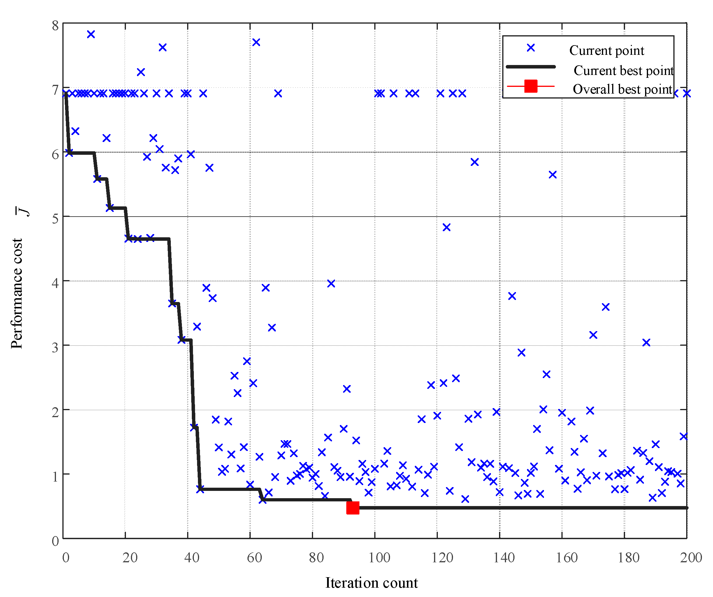
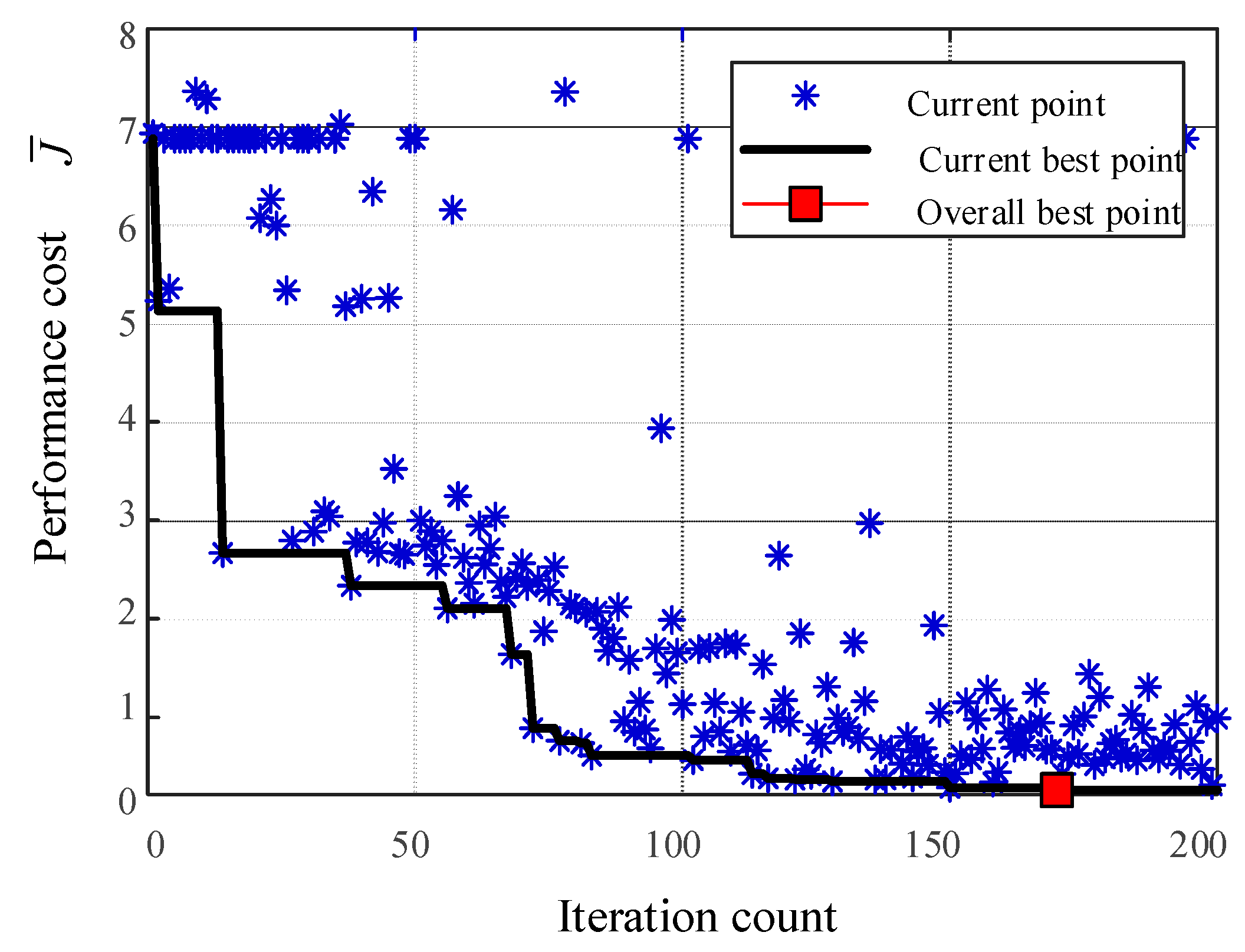
4.2.2. Parameter Tuning by Bayesian Optimization

The next controller’s parameters ( ν i + 1 ,   η i + 1 ) can be selected by maximizing the acquisition function α ( ν ,   η   |   D ) : where Y and X are the domain of ν and η , respectively.
( υ i + 1 , η i + 1 ) = arg max υ Y , η X α ( υ , η | D )
The exploration step chooses a point with a high mean of parameters. The exploitation step chooses a point with a large variance of parameters, which can avoid the algorithm’s falling into local optimal parameters and increase the chance of finding the best performance controller parameters [39,40,41,42,43], i.e.,
α ( υ , η | D ) = E I ( υ , η ) = { ( μ i ( υ , η ) J ^ ) Φ ( Z ) + σ i ( υ , η ) ϕ ( Z ) σ i ( υ , η ) > 0 0 σ i ( υ , η ) = 0
Z = J μ i ( υ , η ) σ i ( υ , η )
where J ^ = min j = 1 , , i J ¯ ( y T , u T ; υ j , η j υ ) is an optimal value for the previous i iterations of the objective function. Φ and ϕ are the probability density function and the cumulative density function of the standard normal distribution, respectively.

5. Simulation and Experiment Results

In this section, the dynamics of a bridge crane is first described. Simulations are provided next to verify the performance of the proposed control method.

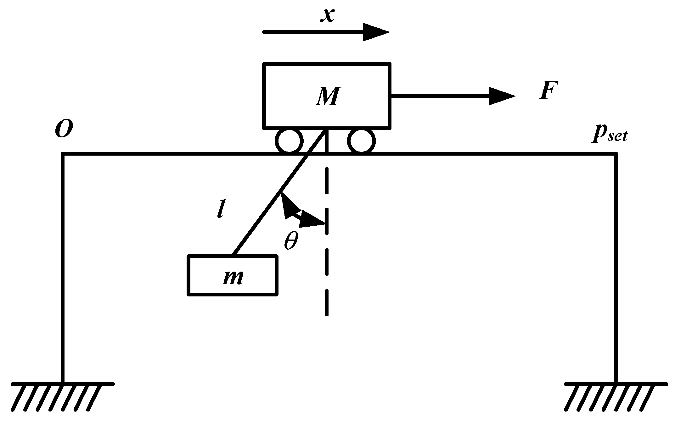
5.1. Bridge Crane Dynamics

A bridge crane is usually composed of wire, payload, and trolley. Its corresponding 2-D simplified physical model is shown in Figure 3 [31,32,33,34,35]. The dynamic equation is defined as follows:
F = ( m + M ) x m l s i n θ m l θ c o s θ 2 m l . θ . c o s θ + m l θ . s i n θ + γ x .
0 = m l 2 θ + 2 m l l . θ m x l c o s θ + m g l s i n θ + ς θ .
where M = 5 Kg and m = 5 Kg denote the mass of trolley and payload, respectively. θ is the vertical direction angle of the payload. g = 9.81 m/s2 represents the gravitational acceleration. l = 1 m is the length of the hoisting rope, which is fixed during transportation. γ = 0 . 1 is the friction between the trolley and the platform. ς = 0 . 1 is the friction between payload and air. F denotes a driving force, and x is the horizontal displacement; O and pset are the trolley’s starting and target points, respectively. According to our method, we do not need to know the dynamic characteristic of a bridge crane. The dynamic Equations (21) and (22) are only used for producing closed-loop experimental data.

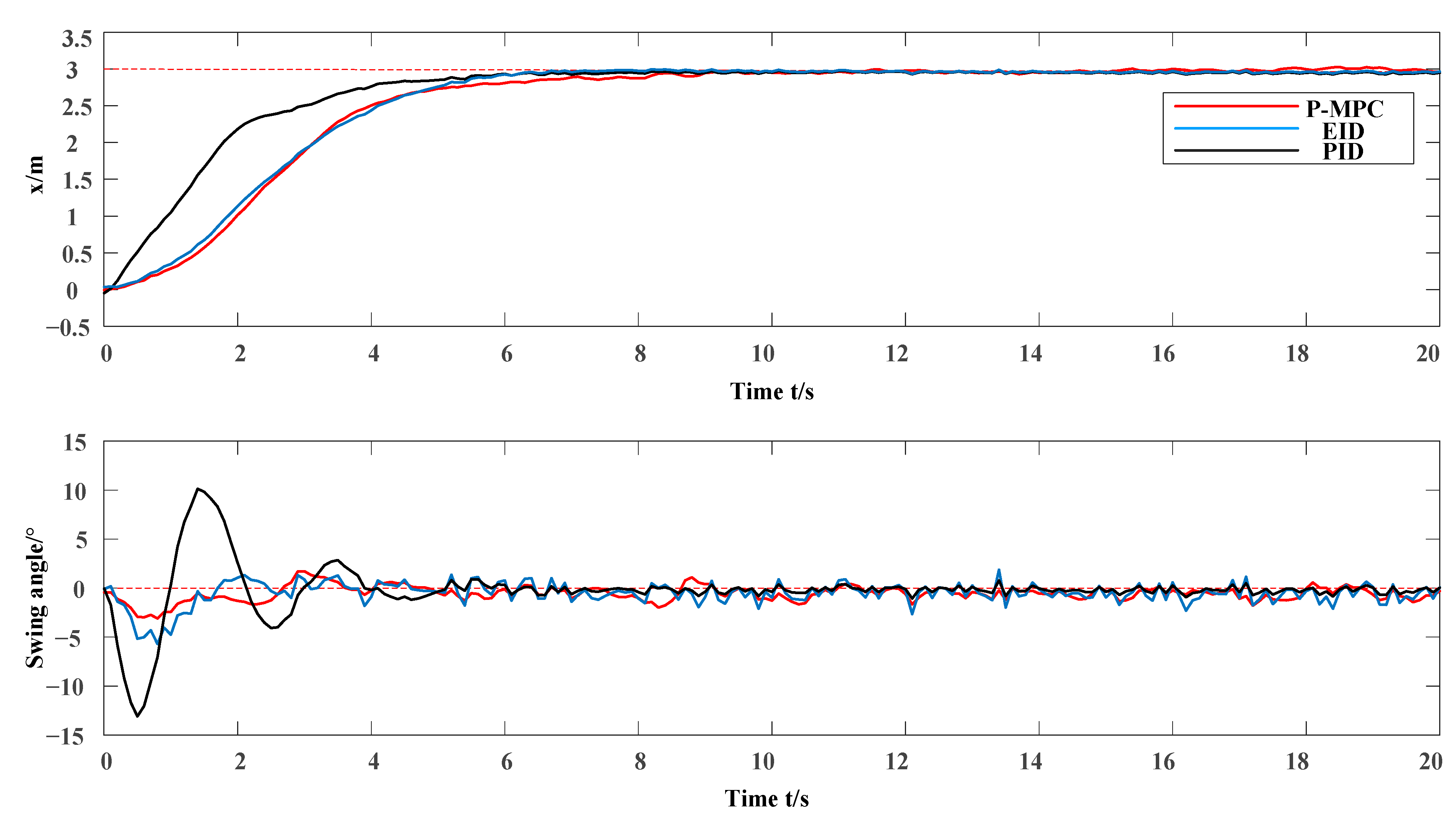
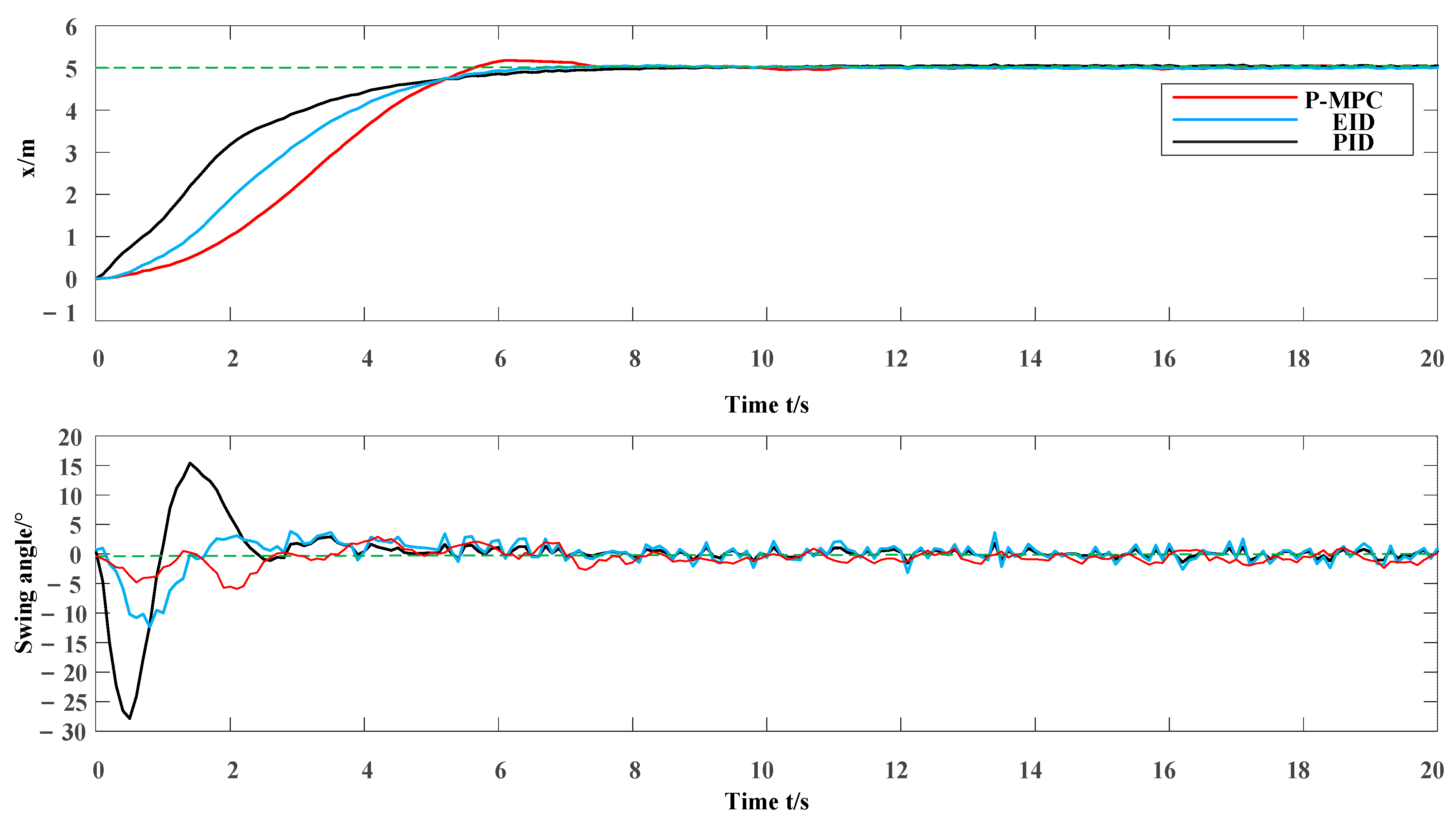
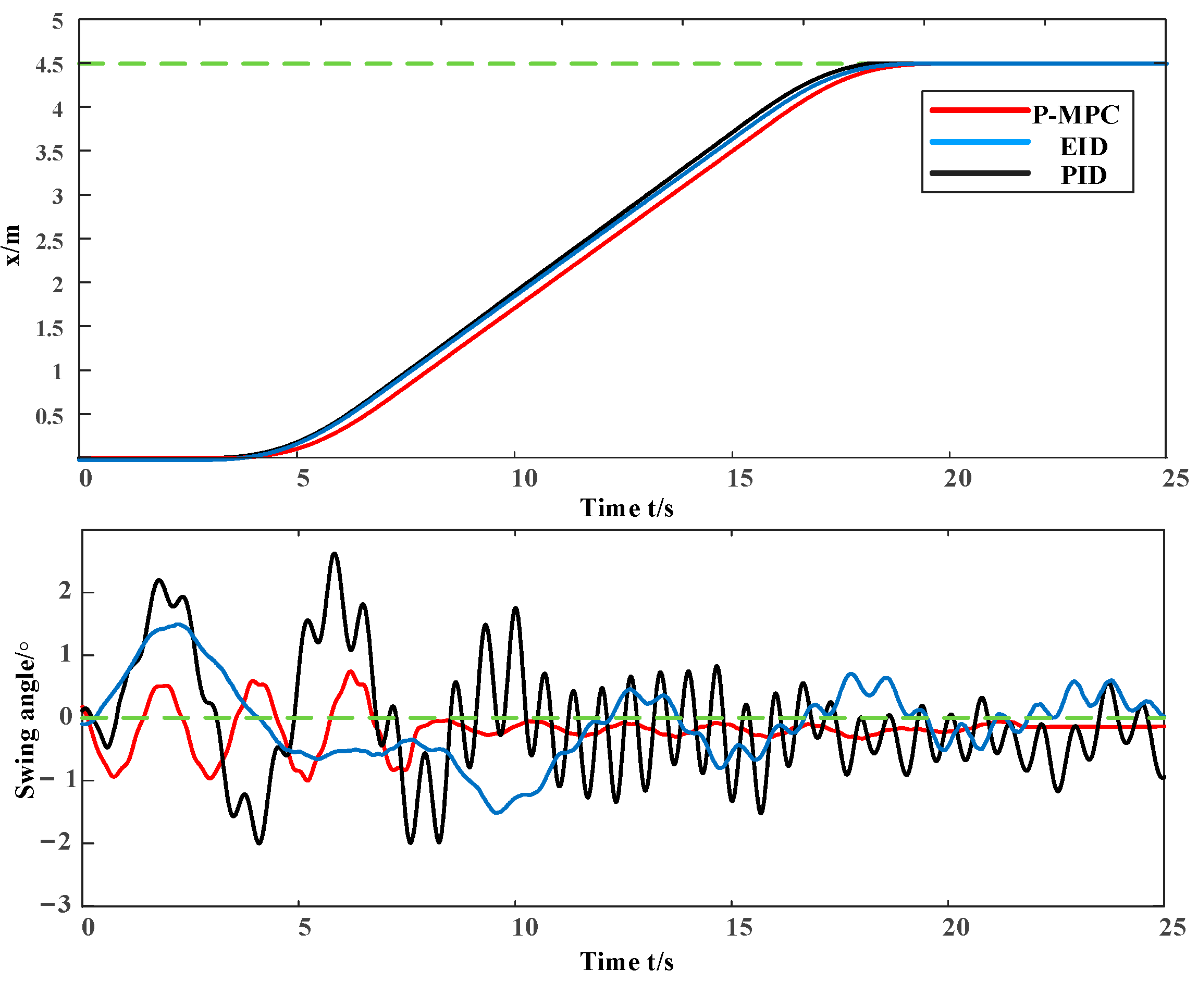
5.2. Simulation Results

MATLAB/Simulink was used to conduct simulations. We conducted 200 closed-loop experiments and collected data for calculating control performance and expanding a historical database. Based on database prior data, we can use BO to optimize the controller parameters. The system is initialized at [ x ( 0 )   x . ( 0 )   θ ( 0 )   θ . ( 0 ) ] = [ 0   0   0   0 ] for each experiment. The sample time is Ts = 0.1 s and TMPC = 1 s (n = 10). The closed-loop performance of each experiment is shown in Figure 4. We set the current test point as a blue cross, the current best point up to iteration i as the black line, and the best closed-loop performance at iteration 92 as a red square. We select the parameters with the best closed-loop performance to verify the algorithm’s feasibility and effectiveness under the following conditions.
Case 1: pset = 3 m.
Case 2: pset = 5 m.
PID and its improved algorithm are currently the primary methods in the application of anti-sway. Model predictive control equivalent input disturbance (EID for short) is currently the best MPC method in the application of anti-sway [35]. Thus performance-driven MPC (P-MPC for short) proposed in this work is compared with the classical double-closed-loop PID (PID for short) [44] and EID.
During the transportation process, the output signals x, θ , and input force F are disturbed by an additive white Gaussian noise.
In the early iteration stage, the closed-loop performance index J ¯ of the system is very large. After accumulating specific closed-loop data, BO can find better parameters. It can be seen from Figure 4 that the performance index decreases faster after the 20th experiment. As the number of experiments increases, the closed-loop performance J ¯ of the experiment becomes lower and lower. The rest of the experiments are focused on the low-cost area. After the 92nd iteration experiments, J ¯ no longer declines. Hence, the parameters at the 92nd can be selected as the best experimental parameters.
From Figure 5 and Figure 6, the swing angle is always within 7° in the entire transportation process of the trolley by using the proposed method. When the trolley reaches the target location, the whole process only takes 8 s. After that, the swing angle oscillates within 2°. The entire transportation process is smooth. The algorithm can restore payload to normal swing quickly while achieving precise positioning and finally maintaining a small angle fluctuation. Besides, the three kinds of approaches of performance comparisons can be seen from Figure 5 and Figure 6. The control performances are shown in Table 1 and Table 2. We can see that P-MPC has the best performance. They all take the same time for the trolley to carry the goods to the target point. In Case 1, the maximum swing angle of PID is 12°. The maximum swing angle of the EID is 7°. The maximum swing angle of P-MPC is only 3.5°, which is significantly smaller than the others. In Case 2, the maximum swing angle of PID is 27°. The maximum swing angle of EID is 12°, and the maximum swing angle of P-MPC is only 7°, which is also much smaller than its two peers. We can compute that the P-MPC method’s closed-loop performance is 0.021 for Case 1 and 0.477 for Case 2, which is much better than its peers 0.366, 0.491 for Case 1 and 0.743, 0.796 for Case 2. Comparing experimental results of the different methods, the proposed P-MPC is the best solution for safety and efficiency in real applications.

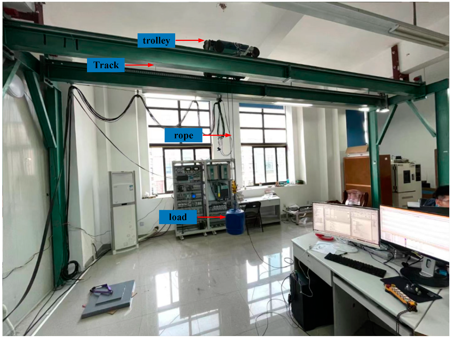
5.3. Experiment Results

A lab was specially built to validate the proposed method, as shown in Figure 7. The experimental platform used three Alternating Current (AC) asynchronous motors to drive the trolley to move on the track. The maximum speed was 0.2 m/s. Due to the limitation of the experimental site, the track length of the crane was 5.5 m, the actual usable length was 5 m, and the maximum lifting rope length was 3 m. The maximum payload mass was 1 t. The moving distance sensor used in this experiment could achieve an accuracy of 1 mm. Using the aircraft altitude angle sensor, the dynamic swing angle and the static swing angle accuracy could reach 0.01°. The friction coefficient was 0.2. The swing angle of the payload was required to remain within ±50 mm after the mechanism stopped in 5 s.
As same as for the simulation, we conducted 200 closed-loop experiments and collected data to calculate the control performance and to expand the historical database. Based on the database prior data, we can use BO to optimize the controller parameters. The system is initialized at [ x ( 0 )   x . ( 0 )   θ ( 0 )   θ . ( 0 ) ] = [ 0   0   0   0 ] for each experiment. The sample time is Ts = 0.003 s and TMPC = 0.03 s (n=10). The closed-loop performance of each experiment is shown in Figure 8. We set the current test point as a blue cross, the current best point up to iteration i as the black line, and the best closed-loop performance at iteration 170 as a red square. Then, we selected the parameters with the best closed-loop performance to verify the algorithm’s feasibility and effectiveness under the following conditions.
Case 3: pset = 4.5 m.
As same as for the simulation, the closed-loop performance index J ¯ of the system is very large in the early iteration stage. After accumulating specific closed-loop data, BO can find better parameters. It can be seen from Figure 8 that the performance index decreases faster after the 15th experiment. As the number of experiments increases, the closed-loop performance J ¯ of the experiment becomes lower and lower. The rest of the experiments are focused on the low-cost area. After the 170th iteration experiment, J ¯ no longer declines. Hence, the parameters at the 170th can be selected as the best experimental parameters.
From Figure 9, the swing angle is always within 1 ° in the entire transportation process of the trolley when using the proposed method. When the trolley reaches the target location, the whole process only takes 20 s. After that, the swing angle oscillates within 0.1°. The entire transportation process is smooth. The algorithm can restore payload to normal swing quickly while achieving precise positioning and finally maintaining a small angle fluctuation. Besides, the three kinds of approaches of performance comparisons can be seen in Figure 9. The control performances are shown in Table 3. We can see that P-MPC has the best performance. They all take the same time for the trolley to carry the goods to the target point. In Case 3, the maximum swing angle of PID is 2.5°. The maximum swing angle of the EID is 1.5°. The maximum swing angle of P-MPC is only 1°, which is significantly smaller than the others. We can compute that the P-MPC method’s closed-loop performance is 0.003 for Case 3, which is much better than its peers 0.015, 0.042 for Case 3. Comparing experimental results of the different methods, the proposed P-MPC is the best solution for safety and efficiency in real applications.

6. Conclusions

This work proposed a performance-driven MPC algorithm for an underactuated 2-D bridge crane system. We could find the best performance MPC controller with predictive model and controller parameters from closed-loop experimental data to deal with unknown dynamic systems. The proposed method can effectively deal with the system’s various constraints that do not cause the controller to saturate. Thus, it is easy to apply it to actual cranes. The simulation results show that this method can achieve high-precision positioning of the trolley and rapid anti-sway of payload, while outperforming the traditional PID controller and EID controller. Our future work will focus on the stability analysis of the proposed method in this paper. We should clarify the least number of closed-loop experiments required to construct a stable and reliable controller. It is necessary to construct a more accurate nonlinear model for large scale cranes, thereby improving the controller’s robustness and stability in application. Our future work aims to promote P-MPC to 3D cranes, carry out a feasibility analysis of optimization results, and focus on chance-constrained stochastic control in the P-MPC framework. The model does not necessarily provide the highest input/output data fit result but yields a good controller corresponding to the best closed-loop performance. Moreover, P-MPC can be extended to solve different control problems, e.g., the inverted pendulum system, the ball and beam system, a translational oscillator with a rotating actuator, and a power-line inspection robot [45,46,47,48]. Engineers who only have little knowledge of control theory can use our method to design a controller with the highly desired performance.

Author Contributions

Conceptualization and methodology, H.B. and Q.K.; writing, H.B.; experiment, J.A. and X.M.; review and editing, M.Z. and Q.K.; supervision, Q.K. and M.Z.; funding acquisition, Q.K. and J.A. All authors have read and agreed to the published version of the manuscript.

Funding

This work was supported in part by the National Natural Science Foundation of China under Grant 51775385, 61703279 and 71371142, the Strategy Research Project of Artificial Intelligence Algorithms of Ministry of Education of China under Grant 000011, and in part by the Fundamental Research Funds for the Central Universities.

Institutional Review Board Statement

Not applicable.

Informed Consent Statement

Not applicable.

Data Availability Statement

Data sharing not applicable.

Acknowledgments

We sincerely acknowledge the previous researchers for their excellent work, which greatly assisted our academic study. Review and editing F.A. Funding acquisition, Q.K., J.A., and F.A. We are also grateful for the efforts from our colleagues in the Sino-German Center of Intelligent Systems, Tongji University.

Conflicts of Interest

The authors declare that there is no conflict of interest regarding the publication of this paper.

References

  1. Vaughan, J.; Kim, D.; Singhose, W. Control of Tower Cranes With Double-Pendulum Payload Dynamics. IEEE Trans. Control Syst. Technol. 2010, 18, 1345–1358. [Google Scholar] [CrossRef]
  2. Sun, N.; Fang, Y.; Chen, H.; Ning, S.; Yongchun, F.; He, C. Adaptive control of underactuated crane systems subject to bridge length limitation and parametric uncertainties. In Proceedings of the 33rd Chinese Control Conference, Nanjing, China, 28–30 July 2014; pp. 3568–3573. [Google Scholar] [CrossRef]
  3. Ye, H. Stabilization of Uncertain Feedforward Nonlinear Systems With Application to Underactuated Systems. IEEE Trans. Autom. Control 2018, 64, 3484–3491. [Google Scholar] [CrossRef]
  4. Wang, J.-J.; Kumbasar, T. Optimal PID control of spatial inverted pendulum with big bang–big crunch optimization. IEEE/CAA J. Autom. Sin. 2018, 7, 822–832. [Google Scholar] [CrossRef]
  5. Yang, T.; Sun, N.; Chen, H.; Fang, Y. Swing suppression and accurate positioning control for underactuated offshore crane systems suffering from disturbances. IEEE/CAA J. Autom. Sin. 2020, 7, 892–900. [Google Scholar] [CrossRef]
  6. Ouyang, H.; Wang, J.; Zhang, G.; Mei, L.; Deng, X. Novel Adaptive Hierarchical Sliding Mode Control for Trajectory Tracking and Load Sway Rejection in Double-Pendulum Overhead Cranes. IEEE Access 2019, 7, 10353–10361. [Google Scholar] [CrossRef]
  7. Li, F.; Zhang, C.; Sun, B. A Minimum-Time Motion Online Planning Method for Underactuated Overhead Crane Systems. IEEE Access 2019, 7, 54586–54594. [Google Scholar] [CrossRef]
  8. He, W.; Ge, S.S. Cooperative control of a nonuniform gantry crane with constrained tension. Automatica 2016, 66, 146–154. [Google Scholar] [CrossRef]
  9. Jaafar, H.I.; Mohamed, Z.; Ramli, L.; Abdullahi, A. Vibration Control of a Nonlinear Double-Pendulum Overhead Crane Using Feedforward Command Shaping. In Proceedings of the 2018 IEEE Conference on Systems, Process and Control, Melaka, Malaysia, 14–15 December 2018; pp. 118–122. [Google Scholar] [CrossRef]
  10. Tysse, G.O.; Cibicik, A.; Egeland, O. Vision-based control of a knuckle boom crane with online cable length estimation. IEEE/ASME Trans. Mechatron. 2020. [Google Scholar] [CrossRef]
  11. Shi, M.; Guo, S.; Jiang, L.; Huang, Z. Active-Passive Combined Control System in Crane Type for Heave Compensation. IEEE Access 2019, 7, 159960–159970. [Google Scholar] [CrossRef]
  12. Tolochko, O.; Bazhutin, D. Anti-Sway Full Order State-Feedback Control of the Overhead Crane with Variable Rope Length Using Luenberger Observer. In Proceedings of the 2018 X International Conference on Electrical Power Drive Systems, Novocherkassk, Russia, 3–6 October 2018; pp. 1–5. [Google Scholar] [CrossRef]
  13. Zhang, M.; Zhang, Y.; Cheng, X. Finite-Time Trajectory Tracking Control for Overhead Crane Systems Subject to Unknown Disturbances. IEEE Access 2019, 7, 55974–55982. [Google Scholar] [CrossRef]
  14. Wu, X.; He, X. Nonlinear Energy-Based Regulation Control of Three-Dimensional Overhead Cranes. IEEE Trans. Autom. Sci. Eng. 2016, 14, 1297–1308. [Google Scholar] [CrossRef]
  15. Doktian, J.; Pongyart, W.; Vanichchanunt, P. Passivity-Based Approach for Overhead Crane Anti-Sway Controller Design. In Proceedings of the 2019 Research, Invention, and Innovation Congress (RI2C), Bankok, Thailand, 11–13 December 2019; pp. 1–4. [Google Scholar] [CrossRef]
  16. Wu, X.; He, X. Enhanced damping-based anti-swing control method for underactuated overhead cranes. IET Control Theory Appl. 2015, 9, 1893–1900. [Google Scholar] [CrossRef]
  17. Sun, Z.; Bi, Y.; Zhao, X.; Sun, Z.; Ying, C.; Tan, S. Type-2 Fuzzy Sliding Mode Anti-Swing Controller Design and Optimization for Overhead Crane. IEEE Access 2018, 6, 51931–51938. [Google Scholar] [CrossRef]
  18. Zhang, M.; Ma, X.; Song, R.; Rong, X.; Tian, G.; Tian, X.; Li, Y. Adaptive Proportional-Derivative Sliding Mode Control Law With Improved Transient Performance for Underactuated Overhead Crane Systems. IEEE/CAA J. Autom. Sin. 2018, 5, 683–690. [Google Scholar] [CrossRef]
  19. He, W.; Zhang, S.; Ge, S.S. Adaptive Control of a Flexible Crane System With the Boundary Output Constraint. IEEE Trans. Ind. Electron. 2013, 61, 4126–4133. [Google Scholar] [CrossRef]
  20. Chwa, D. Sliding-Mode-Control-Based Robust Finite-Time Antisway Tracking Control of 3-D Overhead Cranes. IEEE Trans. Ind. Electron. 2017, 64, 6775–6784. [Google Scholar] [CrossRef]
  21. Ouyang, H.; Hu, J.; Zhang, G.; Mei, L.; Deng, X. Sliding-Mode-Based Trajectory Tracking and Load Sway Suppression Control for Double-Pendulum Overhead Cranes. IEEE Access 2018, 7, 4371–4379. [Google Scholar] [CrossRef]
  22. Lu, B.; Fang, Y.; Sun, N. Continuous Sliding Mode Control Strategy for a Class of Nonlinear Underactuated Systems. IEEE Trans. Autom. Control 2018, 63, 3471–3478. [Google Scholar] [CrossRef]
  23. Gu, X.; Xu, W.; Zhang, M.; Zhang, W.; Wang, Y.; Chen, T. Adaptive Controller Design for Overhead Cranes With Moving Sliding Surface. In Proceedings of the 2019 Chinese Control Conference (CCC), Guangzhou, China, 27–30 July 2019. [Google Scholar] [CrossRef]
  24. Kim, G.-H.; Hong, K.-S. Adaptive Sliding-Mode Control of an Offshore Container Crane With Unknown Disturbances. IEEE/ASME Trans. Mechatron. 2019, 24, 2850–2861. [Google Scholar] [CrossRef]
  25. Jin, G.; Deng, M. Operator-based robust nonlinear free vibration control of a flexible plate with unknown input nonline-arity. IEEE/CAA J. Autom. Sin. 2020, 7, 442–450. [Google Scholar] [CrossRef]
  26. Leite, D.; Aguiar, C.; Pereira, D.A.; Souza, G.; Skrjanc, I. Nonlinear Fuzzy State-Space Modeling and LMI Fuzzy Control of Overhead Cranes. In Proceedings of the IEEE International Conference on Fuzzy Systems, New Orleans, LA, USA, 18–21 June 2019; pp. 1–6. [Google Scholar] [CrossRef]
  27. Sun, Z.; Ling, Y.; Sun, Z.; Bi, Y.; Tan, S.; Ding, L. Designing and Application of Fuzzy PID Control for Overhead Crane Systems. In Proceedings of the 2019 2nd International Conference on Information Systems and Computer Aided Education (ICISCAE), Dalian, China, 28–30 September 2019; pp. 411–414. [Google Scholar]
  28. Das, S.; Dhalmahapatra, K.; Maroo, P.; Maiti, J. A self-tuning neuromorphic controller to minimize swing angle for overhead cranes. In Proceedings of the 2018 4th International Conference on Recent Advances in Information Technology (RAIT), Dhanbad, India, 15–17 March 2018; pp. 1–6. [Google Scholar]
  29. Wang, D.; He, H.; Liu, D. Intelligent Optimal Control With Critic Learning for a Nonlinear Overhead Crane System. IEEE Trans. Ind. Inform. 2017, 14, 2932–2940. [Google Scholar] [CrossRef]
  30. Chen, H.; Fang, Y.; Sun, N. A Swing Constraint Guaranteed MPC Algorithm for Underactuated Overhead Cranes. IEEE/ASME Trans. Mechatron. 2016, 21, 2543–2555. [Google Scholar] [CrossRef]
  31. He, X.; He, W.; Shi, J.; Sun, C. Boundary Vibration Control of Variable Length Crane Systems in Two-Dimensional Space With Output Constraints. IEEE/ASME Trans. Mechatron. 2017, 22, 1952–1962. [Google Scholar] [CrossRef]
  32. Giacomelli, M.; Faroni, M.; Gorni, D.; Marini, A.; Simoni, L.; Visioli, A. MPC-PID control of operator-in-the-loop overhead cranes: A practical approach. In Proceedings of the 2018 7th International Conference on Systems and Control (ICSC), Valencia, Spain, 24–26 October 2018; pp. 321–326. [Google Scholar] [CrossRef] [Green Version]
  33. Zhu, Y.; Niu, D.; Li, Q.; Chen, Y.; Wei, S.; Liu, J. Anti-shake positioning algorithm of bridge crane based on phase plane analysis. J. Eng. 2019, 2019, 8370–8373. [Google Scholar] [CrossRef]
  34. Giacomelli, M.; Colombo, D.; Faroni, M.; Schmidt, O.; Simoni, L.; Visioli, A. Comparison of Linear and Nonlinear MPC on Operator-In-the-Loop Overhead Cranes. In Proceedings of the 7th International Conference on Control, Mechatronics and Automation (ICCMA), Delft, The Netherlands, 6–8 November 2019; pp. 221–225. [Google Scholar] [CrossRef] [Green Version]
  35. Ma, X.; Bao, H. An Anti-Swing Closed-Loop Control Strategy for Overhead Cranes. Appl. Sci. 2018, 8, 1463. [Google Scholar] [CrossRef] [Green Version]
  36. Bansal, S.; Calandra, R.; Xiao, T.; Levine, S.; Tomlin, C.J. Goal-driven dynamics learning via Bayesian optimization. In Proceedings of the IEEE 56th Annual Conference on Decision and Control (CDC), Melbourne, VIC, Australia, 12–15 December 2017; pp. 5168–5173. [Google Scholar] [CrossRef] [Green Version]
  37. Bao, H.; An, J.; Zhou, M.; Kang, Q. A Data-driven MPC Algorithm for Bridge Cranes. In Proceedings of the 2020 International Conference on Advanced Mechatronic Systems (ICAMechS), Hanoi, Vietnam, 10–13 December 2020; pp. 328–332. [Google Scholar]
  38. Yue, M.; Hou, X.; Fan, M.; Jia, R. Coordinated trajectory tracking control for an underactuated tractor-trailer vehicle via MPC and SMC approaches. In Proceedings of the 2017 2nd International Conference on Advanced Robotics and Mechatronics (ICARM), Hefei and Tai’an, China, 27–31 August 2017; pp. 82–87. [Google Scholar] [CrossRef]
  39. Shi, X.D.; Kang, Q.; Zhou, M.C.; Abusorrah, A.; An, J. Soft Sensing of Nonlinear and Multimode Processes based on Semi-supervised Weighted Gaussian Regression. IEEE Sens. J. 2020, 20. [Google Scholar] [CrossRef]
  40. Shi, X.; Kang, Q.; Zhou, M.; An, J.; Abusorrah, A. Novel L1 Regularized Extreme Learning Machine for Soft-sensing of an Industrial Process. IEEE Trans. Ind. Inform. 2021. [Google Scholar] [CrossRef]
  41. Carr, S.; Garnett, R.; Lo, C. BASC: Applying Bayesian optimization to the search for global minima on potential energy surfaces. In Proceedings of the International Conference on Machine Learning (ICML), New York, NY, USA, 18–24 June 2016; pp. 898–907. [Google Scholar]
  42. Wang, X.; Kang, Q.; Zhou, M.; Pan, L.; Abusorrah, A. Multiscale Drift Detection Test to Enable Fast Learning in Nonsta-tionary Environments. IEEE Trans. Cybern. 2021, 51, 3483–3495. [Google Scholar] [CrossRef] [PubMed]
  43. Kang, Q.; Song, X.; Zhou, M.; Li, L. A Collaborative Resource Allocation Strategy for Decomposition-based Multi-objective Evolutionary Algorithms. IEEE Trans. Syst. Man Cybern. Syst. 2019, 49, 2416–2423. [Google Scholar] [CrossRef]
  44. Sun, N.; Yang, T.; Fang, Y.; Wu, Y.; Chen, H. Transportation Control of Double-Pendulum Cranes with a Nonlinear Qua-si-PID Scheme: Design and Experiments. IEEE Trans. Syst. Man Cybern. Syst. 2019, 49, 1408–1418. [Google Scholar] [CrossRef]
  45. Dian, S.; Chen, L.; Hoang, S.; Pu, M.; Liu, J. Dynamic balance control based on an adaptive gain-scheduled backstepping scheme for power-line inspection robots. IEEE/CAA J. Autom. Sin. 2017, 6, 198–208. [Google Scholar] [CrossRef]
  46. Deng, K.; Sun, Y.; Li, S.; Lu, Y.; Brouwer, J.; Mehta, P.G.; Zhou, M.; Chakraborty, A. Model Predictive Control of Central Chiller Plant With Thermal Energy Storage Via Dynamic Programming and Mixed-Integer Linear Programming. IEEE Trans. Autom. Sci. Eng. 2014, 12, 565–579. [Google Scholar] [CrossRef] [Green Version]
  47. Li, S.; Zhou, M.; Luo, X. Modified Primal-Dual Neural Networks for Motion Control of Redundant Manip-ulators with Dynamic Rejection of Harmonic Noises. IEEE Trans. Neural Netw. Learn. Syst. 2018, 29, 4791–4801. [Google Scholar] [CrossRef] [PubMed]
  48. Cao, Z.; Xiao, Q.; Huang, R.; Zhou, M. Robust Neuro-Optimal Control of Underactuated Snake Robots With Experience Replay. IEEE Trans. Neural Netw. Learn. Syst. 2017, 29, 208–217. [Google Scholar] [CrossRef] [PubMed]
Figure 1. Performance-driven MPC algorithm framework.
Machines 09 00177 g001
Figure 2. Proposed dual-layer control architecture.
Machines 09 00177 g002
Figure 3. 2-D model of a bridge crane.
Machines 09 00177 g003
Figure 4. Performance-driven parameter tuning.
Machines 09 00177 g004
Figure 5. Result of Case 1.
Machines 09 00177 g005
Figure 6. Result of Case 2.
Machines 09 00177 g006
Figure 7. Main mechanical structure of the laboratory-scale overhead crane.
Machines 09 00177 g007
Figure 8. Performance-driven parameter tuning.
Machines 09 00177 g008
Figure 9. Result of Case 3.
Machines 09 00177 g009
Table 1. The Comparison of the Three Approaches for Case 1.
ApproachesMaximum Swing AngleTransporting
Time
Closed-Loop
Performance
P-MPC3.5°8 s0.021
EID8 s0.366
PID12°8 s0.491
Table 2. The Comparison of the Three Approaches for Case 2.
ApproachesMaximum Swing AngleTransporting
Time
Closed-Loop
Performance
P-MPC8 s0.477
EID12°8 s0.743
PID27°8 s0.796
Table 3. The Comparison of the Three Approaches for Case 3.
ApproachesMaximum Swing AngleTransporting
Time
Closed-Loop
Performance
P-MPC1.0°20 s0.003
EID1.5°20 s0.015
PID2.5°20 s0.042
Publisher’s Note: MDPI stays neutral with regard to jurisdictional claims in published maps and institutional affiliations.

