Aeroacoustic Optimization of the Bionic Leading Edge of a Typical Blade for Performance Improvement

Abstract

New, innovative optimization approaches to improve turbomachine performance and reduce turbomachine noise are significant in engineering. In this paper, based on the bionic concept, a wave structure is used to shape the leading edge of the blade. Using an NACA0018 blade as the basic blade, a united parametric approach controlled by three parameters is proposed to configure the wavy leading edge. Then, a new optimization strategy boosting design efficiency is established to output the optimal design results. Finally, the corresponding performance and flow mechanism are analyzed. Taking into account the existence of the hub wall and the shroud wall from the closed impeller, a near-wall adjustment factor is added, the significance of which is herein demonstrated. An optimal bionic blade is successfully obtained by the optimization strategy, which can reduce the mean drag coefficient by about 6% and the overall sound pressure level by about 3 dB, in relative to the original blade. Mechanism analysis revealed that the wave structure can induce spanwise velocity at the leading edge and cause a further delay in flow separation in the downstream region, synchronously reducing drag and noise.

1. Introduction

Turbomachinery plays an important role in national economic development; many scholars have already carried out a lot of research in the field [1,2,3]. As a hot topic, the control of turbomachinery noise is particularly important for operational stability and comfort of the working environment. Sandra [4] and Carlo [5] predicted tonal noise in centrifugal fans by experimental and numerical simulation, and found that the blade is one of the noise sources in turbomachinery. The blade’s shape is closely related to performance and noise. This paper proposes a new blade design strategy to improve turbomachine performance and reduce turbomachine noise.

In recent years, the concept of bionics has been widely adopted in various fields [6,7,8]. Graham [9] studied the mechanism whereby owls fly quietly and found that the peculiarities of owl feathers (the leading edge comb, the downy upper surface, and the trailing edge fringe) are important factors. Among the peculiarities of the leading edge comb, leading-edge protuberance has been studied in different fields. In aviation, Chen [10,11] found that the wavy leading edge can reduce the drag fluctuation and noise of the airfoil through numerical calculation and experiments. In the marine field, Gao [12] studied the effect of leading-edge protuberances on the rudder, and found that protuberances had drag reduction ability. In the mechanical field, Tong [13] applied leading-edge protuberances to the vanes of axial fans, and concluded that fan efficiency was improved and fan noise was reduced. For the wavy parameters of the leading edge, currently, only two parameters have been proposed, namely, wavelength (or wavenumber) and amplitude (shown in Figure 1a). Lyu [14] found that the larger the amplitude and the smaller the wavelength, the more obvious is the noise reduction effect in a certain range.

The above literature show that it is important to study the wavy leading edge of blades in turbomachinery. Most of the related research mainly has focused on the comparison between original leading edge and wavy leading edge; thus, the related parameter optimization needs to be supplemented. As presented in Figure 1b, for turbomachinery, the impeller is mainly divided into closed impeller, semi-open impeller, and open impeller. However, for the closed impeller, only the two parameters (wavelength and amplitude) that determine the wavy shape are not enough. As shown in Figure 1c, the blade is installed between the hub wall and the shroud wall. It has been found that the near-wall shape of the blade plays a significant role in determining flow stability. Hence, a near-wall adjustment factor is proposed in this study, which can adjust the wavy install location near the hub and shroud walls.

The main purpose of this paper is to propose a new optimization strategy for the wavy leading edge of turbomachinery blades. Based on previously settled variables, a newly proposed near-wall adjustment factor is considered in this paper, and the corresponding composite effects are herein investigated. Using the NACA0018 blade (attack angle α = 0°) as the basic blade, a new optimization strategy was proposed, including the parametric design approach and Box-Behnken Design (BBD). Most importantly, the effects of the wavy leading edge on performance and noise were investigated and clarified during the optimization process. The study is organized as follows: Section 2 illustrates the numerical approach and its validation; Section 3 introduces the newly developed parametric approach and proposes the bionic optimization strategy; Section 4 analyzes the results of the original blade and the optimized blade, and the corresponding mechanism; Section 5 provides the conclusions.

2. Numerical Method

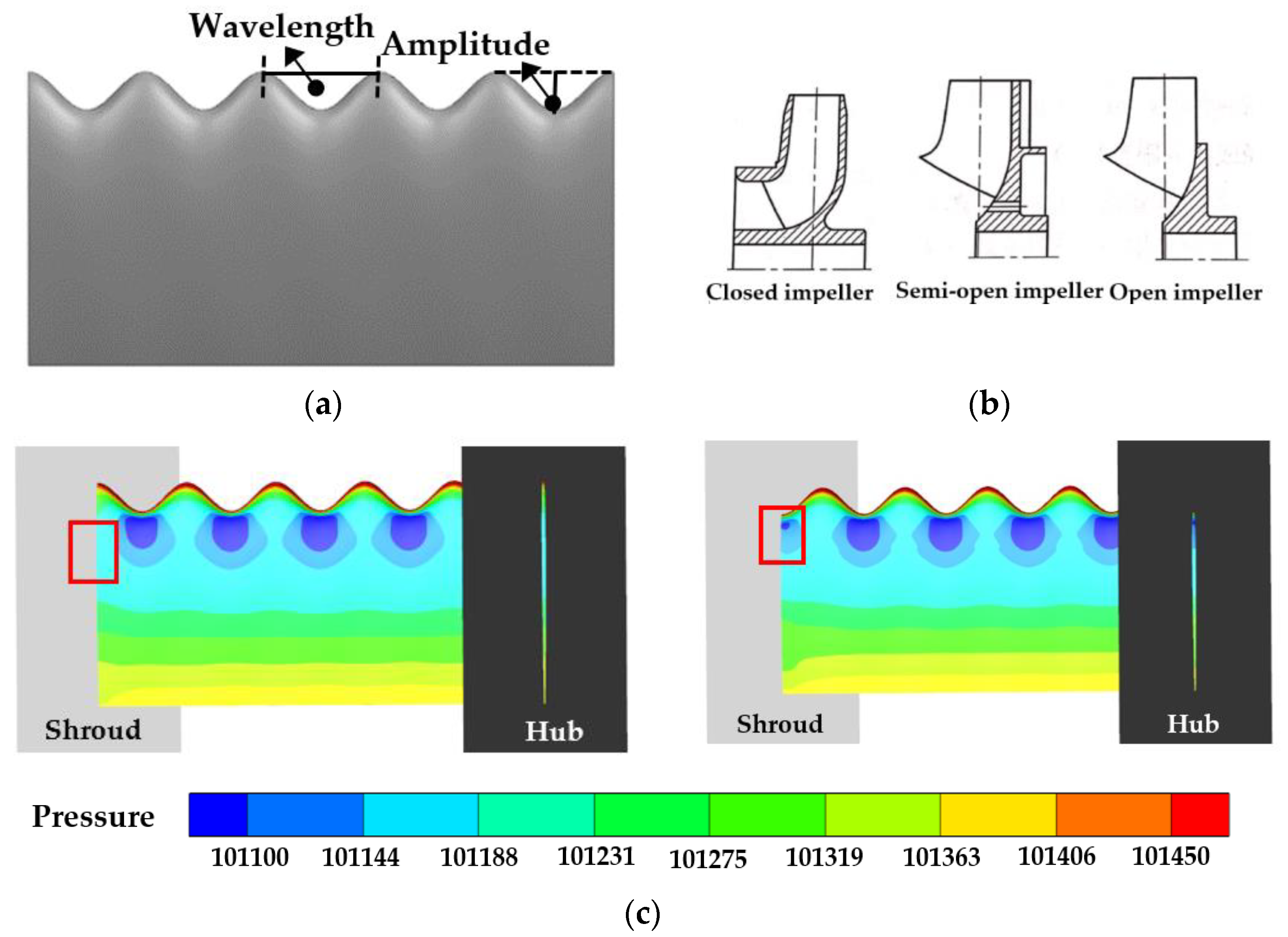
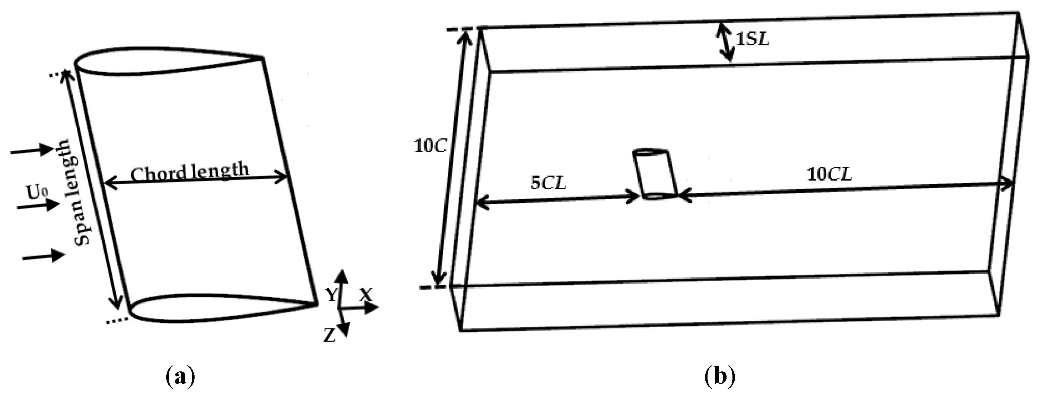
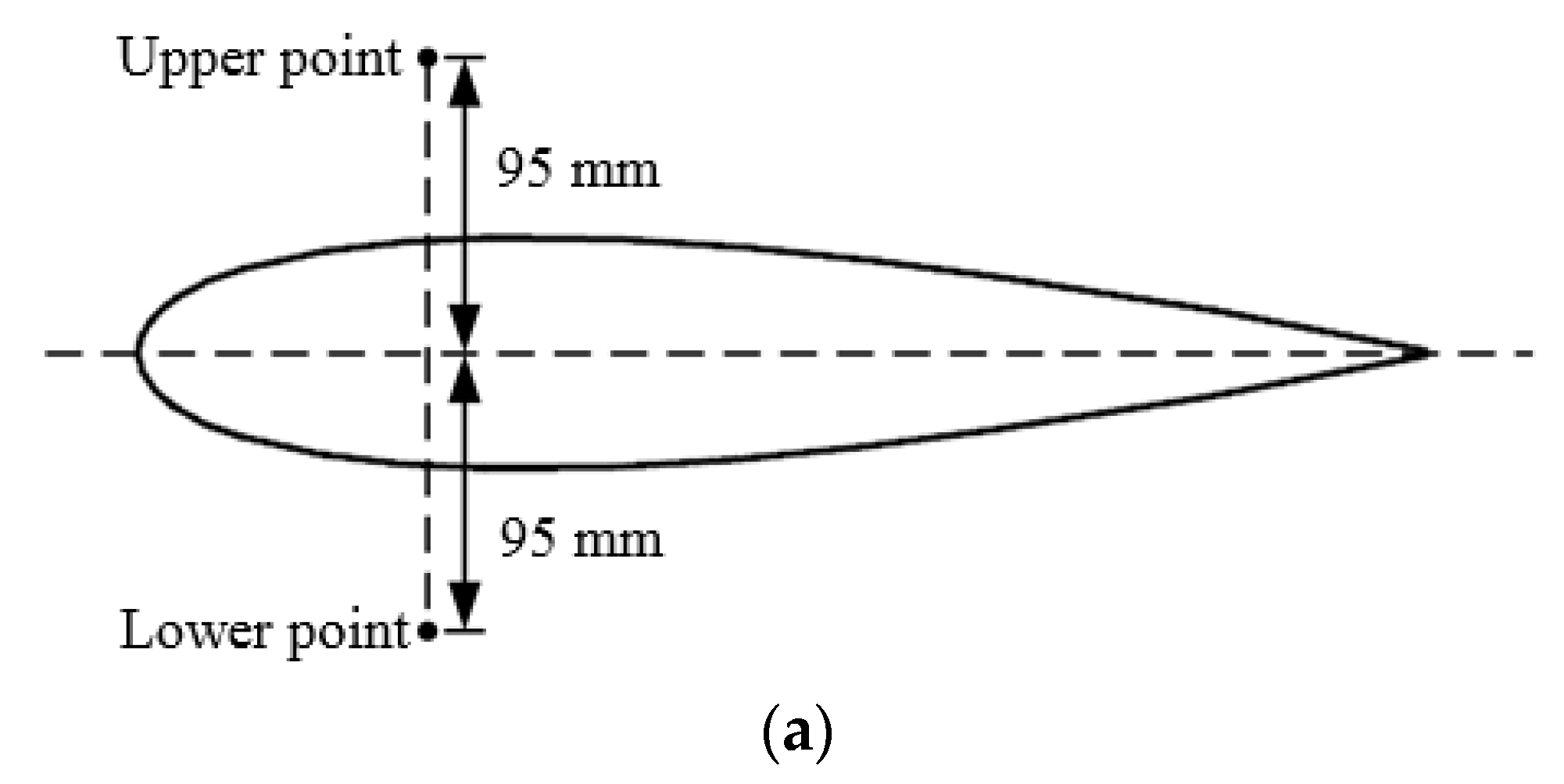
2.1. Investigation Object

In the field of turbomachinery, many scholars [15,16,17] have used the typical NACA blade in related research. To verify the accuracy of the numerical approach by comparing the calculation result with experimental data, taking into account the existing experimental data of relevant NACA [18,19], the NACA0018 blade was taken as the study target in this paper. For some impellers and vanes, the circumferential distribution of blades is relatively sparse, such as the water jet pump’s impeller/vane [20] and the nuclear coolant pump’s impeller [21]. Besides, as a basic work for the bionic design of closed impellers, this study seeks to provide a technical reference for the performance improvement of turbomachinery. Therefore, a single NACA0018 blade is studied instead of a blade cascade in this paper.

As shown in Figure 2a, for the NACA0018 blade, the chord length is CL = 100 mm and the span length is SL = 200 mm. According to the experimental condition [19], the Reynolds number is Re = 1.6 × 10⁵ in this study, the corresponding flow speed of which is U_o = 24 m/s via the conversion formula.

Figure 2b shows the calculation domain. The inlet boundary is placed 5 CL upstream of the leading edge of the NACA blade, and the outlet boundary is set to be 10 CL downstream of the trailing edge of the NACA blade, which can allow the flow development in the wake to be fuller. Considering the closed impeller structure, the spanwise length in the Z-direction is placed 1 SL, and the spanwise wall of the calculation domain can be seen as the hub wall and shroud wall of the closed impeller.

2.2. Simulation Method and Boundary Conditions

For the flow field calculation, a turbulence model is introduced to solve the continuity and momentum transport equations, and for the far-field sound calculation, a hybrid method of CFD (Computational Fluid Dynamics) and CA (Computational Acoustics) is employed. All solving processes are executed in the ANSYS-FLUENT solver.

The boundary conditions are set as follows: the inlet boundary is velocity (U_o = 24 m/s); the outlet boundary is pressure (P_out = 1 atm); other boundaries are non-slip walls. The medium is air. For the steady calculation, the turbulence model is the Shear Stress Transport k-ω (SST k-ω) model; for the unsteady calculation, the large-eddy simulation is introduced to solve the time-dependent turbulent flow; for the sound field calculation, the Ffowcs Williams-Hawkings (FW-H) equation is added to the aerodynamic performance simulation after the flow field simulation. To solve the Navier–Stokes equations, the SIMPLEC algorithm is applied, which can result in convergence more quickly for the pressure-velocity coupling [22].

2.2.1. Large-Eddy Simulation

The large-scale and small-scale vortices are separated by the spatial filter function in Large Eddy Simulation (LES), which can be expressed as [23]:

$$\overline{F}(x)={\displaystyle {\int }_{D}G(x-z,\Delta )}F(z)dz$$

(1)

where G is the Gaussian filter, F is the variable, $\Delta$ is the subgrid characteristic length scale, D is the domain of concern. The large-scale vortices (larger than $\Delta$) are directly simulated and the small-scale vortices (smaller than $\Delta$) are filtered out.

For the low Mach number of 0.07, medium can be considered the incompressible flow. After filtering the continuity equation and momentum transport equation, the filter equation for incompressible fluid can be obtained as:

$$\frac{\partial \overline{u_i}}{\partial x_i}=0$$

(2)

$$\frac{\partial \overline{u_i}}{\partial t}+\frac{\partial }{\partial x_j}(\overline{u_i}\overline{u_j})=-\frac{1}{\rho }\frac{\partial \overline{P}}{\partial x_i}+\upsilon \frac{\partial }{\partial x_j}(\frac{\overline{u_j}}{\partial x_j})+\frac{\partial \left(\overline{{\tau }_{ij}}\right)}{\partial x_j}$$

(3)

where $\overline{u_i}$ and $\overline{u_j}$ are the average velocity component after the filtering operation; $\upsilon$ is the kinematic viscosity; $\rho$ is the fluid density; $\overline{P}$ is the grid-scale static pressure; $\overline{{\tau }_{ij}}=(\overline{u_i}\overline{u_j}-\overline{u_i{u}_j})$ is the Subgrid-scale Reynolds stress tensor. The Subgrid-scale Reynolds stress tensor is expressed by an eddy-viscosity assumption:

$$\overline{{\tau }_{ij}}=2{\upsilon }_t\overline{S_{ij}}-\frac{1}{3}{\delta }_{ij}\overline{{\tau }_{kk}}={\upsilon }_t(\frac{\partial \overline{u_i}}{\partial x_j}+\frac{\partial \overline{u_j}}{\partial x_i})-\frac{1}{3}{\delta }_{ij}\overline{{\tau }_{kk}}$$

(4)

where ${\upsilon }_t$ is the eddy-viscosity; ${\delta }_{ij}$ is the strain rate tensor at the solution scale; $\overline{S_{ij}}$ is the deformation tensor of the resolved field.

To solve the system of Equations (3)–(5), the Wall-Adapting Local Eddy-viscosity (WALE) model is introduced, which is determined as:

$${\upsilon }_t={(C_w\Delta )}^2\frac{{(S_{ij}^d{S}_{ij}^d)}^{3/2}}{{\left(\overline{S_{ij}}\overline{S_{ij}}\right)}^{5/2}+{(S_{ij}^d{S}_{ij}^d)}^{5/4}}$$

(5)

where $S_{ij}^d=\frac{1}{2}({\overline{g}}_{ij}^2+{\overline{g}}_{ji}^2)-\frac{1}{3}{\delta }_{ij}{\overline{g}}_{kk}^2$; $C_w$ is a constant.

2.2.2. Ffowcs Williams–Hawkings Equation

For the acoustic simulation, the FW–H equation was proposed by Ffowcs Williams and Hawkings [24]:

$$\frac{1}{c_0^2}\frac{{\partial }^2{p}^{\prime }}{\partial t^2}-{\nabla }^2{p}^{\prime }=\frac{\partial }{\partial t}\left\{\left[{\rho }_0{v}_n+\rho (u_n-v_n)\right]\delta \left(f\right)\right\}-\frac{\partial }{\partial x_i}\left\{\left[P_{ij}{n}_j+\rho u_i(u_n-v_n)\right]\delta \left(f\right)\right\}+\frac{{\partial }^2}{\partial x_i\partial x_j}\left[T_{ij}H\left(f\right)\right]$$

(6)

where $p^{\prime }=(p-p_0)$ is the sound pressure of the disturbed flow field, ${\rho }_0$ is the undisturbed fluid density, $\rho$ is the disturbed fluid density, $c_0$ is the reference sound speed, $u_i$ stands for the component of the fluid tangential velocity in the $x_i$ direction, $u_n$ stands for the outward normal from $f$ of fluid velocity, $f$ is the wall function, $v_n$ stands for the outward normal on the wall, $\delta \left(f\right)$ and $H\left(f\right)$ represent the Dirac delta function and the Heaviside function, $P_{ij}$ is the compressible stress tensor, $T_{ij}=\rho u_i{u}_j+P_{ij}-c^2\left(\rho -{\rho }_0\right){\delta }_{ij}$ is the Lighthill stress tensor.

For the FW–H equation, the left side of the equation is the sound field information, and the right side of the equation is the sound source information. The sound source information is mainly composed of a monopole, dipole, and quadrupole. When the sound source is determined, the sound field is also obtained. According to reference [25], the dipole is the main sound source for the NACA0018 blade, so the solid surface of the blade is used as the dipole in this paper.

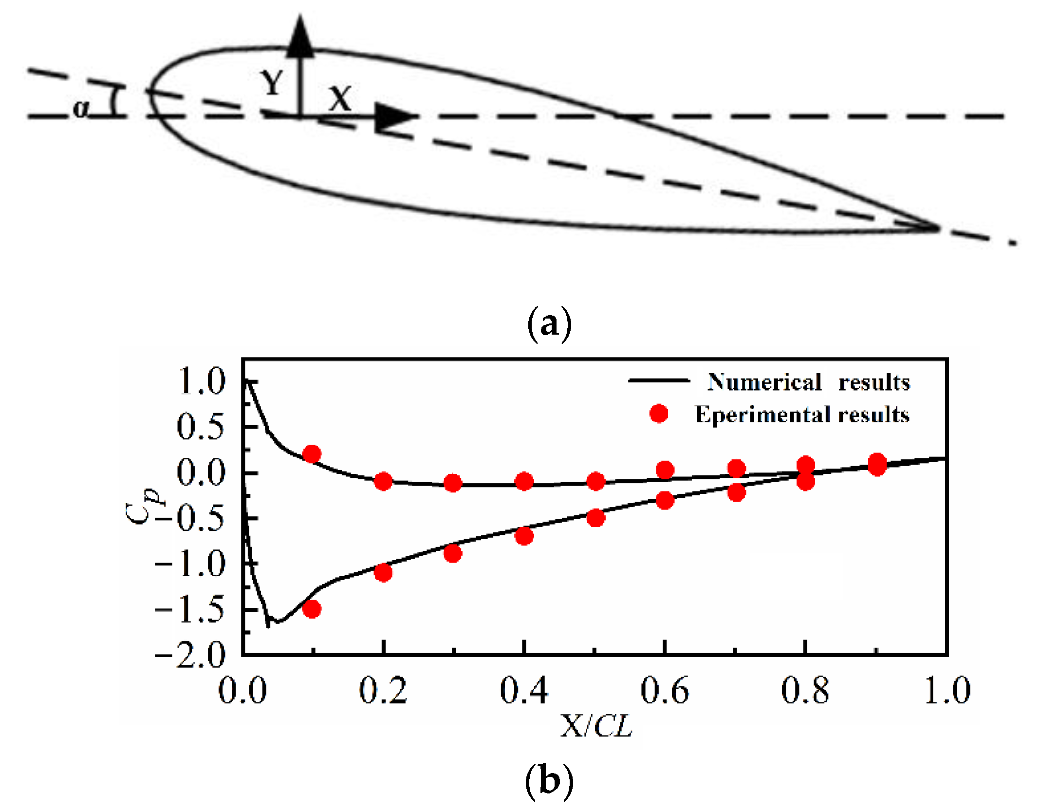
2.3. Numerical Method Validation

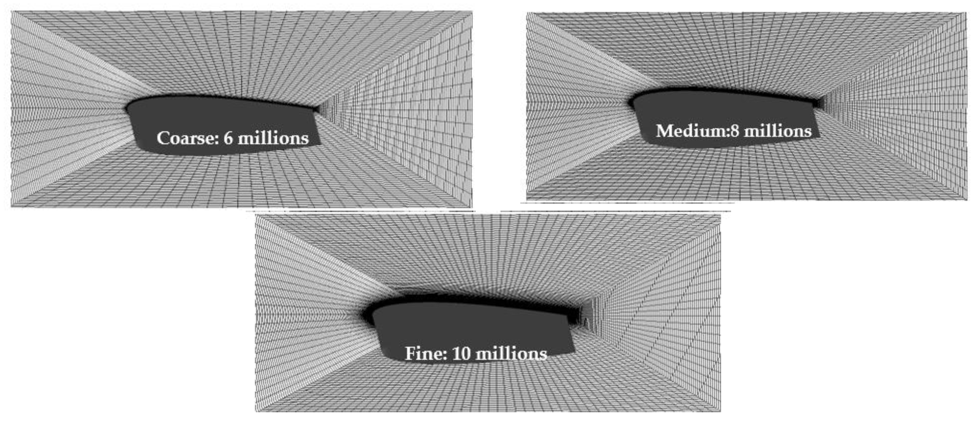
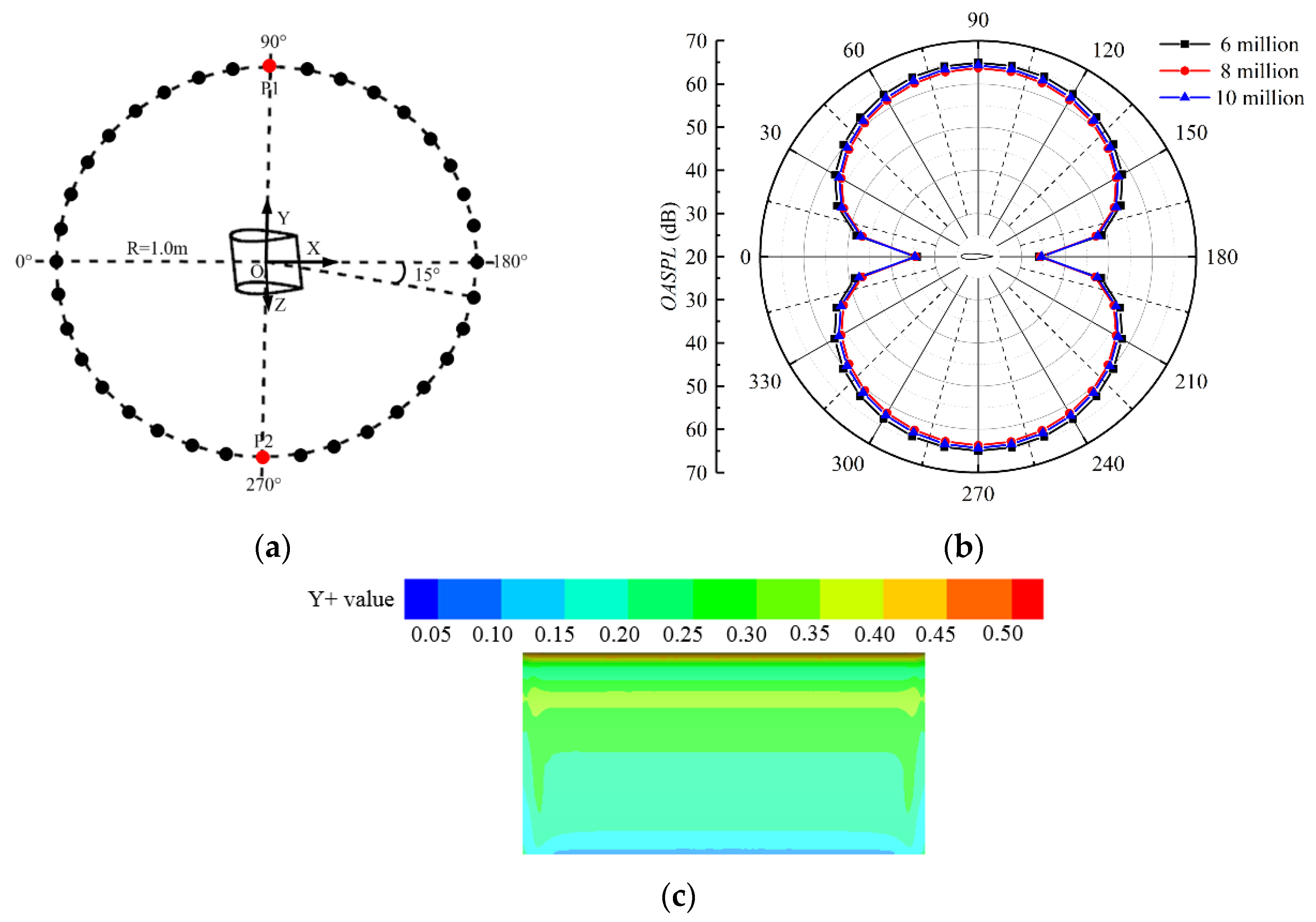
2.3.1. Mesh Independence

A finite volume method was employed in the simulation process, so the influence of the mesh parameters on the performance predictions needs to be excluded. Three meshing schemes (coarse, medium, and fine) were generated for mesh independent validation; the partial enlarged drawing and total number of the schemes are given in Figure 3. The calculation domain is divided by the hexahedral mesh and the O-grid topology is used in the near-blade domain.

The overall sound pressure level (OASPL) with the coarse, medium, and fine grids are compared to each other at the monitoring points in the Y-direction. As shown in Figure 4a, the monitoring points were evenly distributed in the Y-direction, the center of which is the airfoil’s centroid and the radius of which is 1.0 m. The OASPL is one of the evaluation criteria for the noise, the expression of which is determined in Equation (7):

$$OASPL=10\times \lg (\frac{{\displaystyle \sum _{i=1}^n{p}_i^2}}{p_{ref}^2})$$

(7)

where pref is the reference pressure, whose value is 2 × 10⁻⁵ Pa (for air); p_i is the effective sound pressure of different frequency, which can be calculated via the FW–H equation. Thus, the sound field results of three grid schemes at the monitoring points are given in Figure 4b, and it can be found that the increased mesh density has little influence on the sound field calculation after the medium girds. Considering the balance of calculation time and accuracy, the scheme of medium grids is the best.

Besides, to ensure that the medium girds are suitable for the LES, the Y + value should be below 1. Thus, the Y+ value of the blade surface is given in Figure 4c, and it was found out that the Y + value is less than 1. Overall, the scheme of medium grids can be applied to the numerical method.

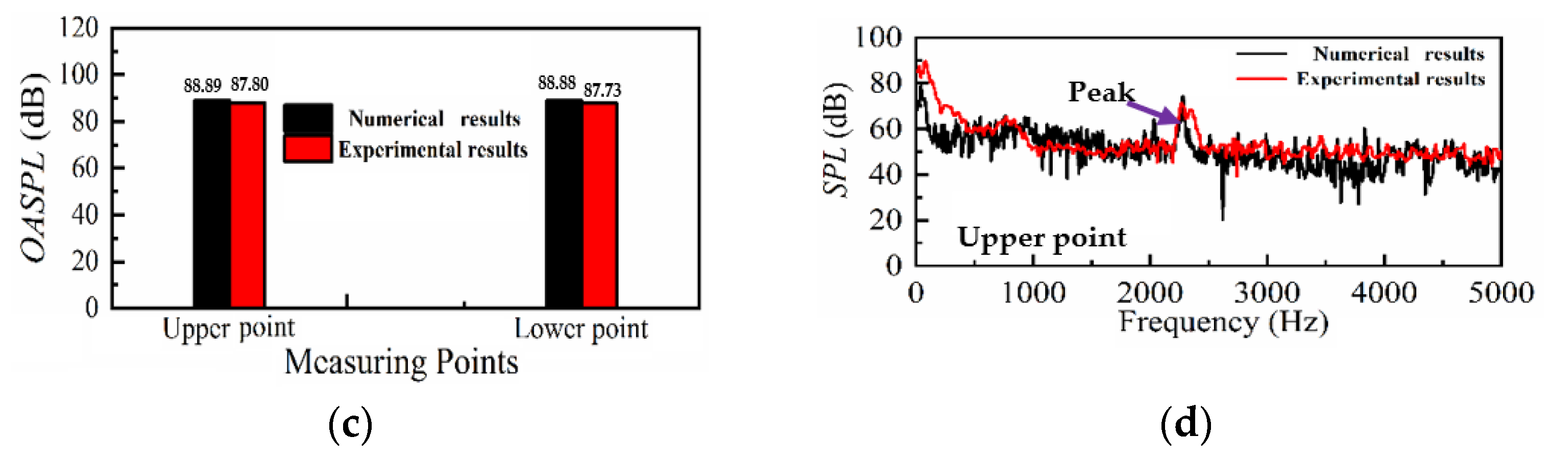
2.3.2. Experimental and Numerical Comparison

According to the relevant experimental data of NACA0018 [18,19], the numerical method was verified from aerodynamic and acoustic performance.

For the aerodynamic performance, the time-averaged pressure coefficient (C_p) along the NACA0018 blade at attack angle α = 6° (Figure 5a) is measured [18], which is determined as in Equation (8):

$$C_p=\frac{(p-p_{\infty })}{0.5{\rho }_0{U}_{\infty }^2}$$

(8)

where $P$ is the static pressure, $P_{\infty }$ is the undisturbed static pressure, ${\rho }_0$ is the medium density, $U_{\infty }$ is the incoming flow velocity.

Thus, based on the experimental condition [18], the pressure coefficient is calculated by the simulation method described in Section 2.2. A comparison of the experimental and numerical results on pressure distribution is given in Figure 5b. The overall pressure distribution along the NACA0018 blade is the same that of the experiment.

For the acoustic performance, the OASPL and Sound Pressure Level (SPL) at the upper and lower surface of the NACA0018 blade (α = 6°) are measured [19], which is given in Figure 6a. The SPL is determined as in Equation (9):

$$SPL=20\lg \left(\frac{P_e}{P_{ref}}\right)$$

(9)

where p_ref is the reference pressure, whose value is 2 × 10⁻⁵ Pa (for air); p_e is the effective sound pressure.

According to the experimental condition [19], the OASPL and the SPL are calculated by the simulation method of Section 2.2. As shown in Figure 6b, it can meet the accuracy standard [26] that the errors of the upper point and lower point were both controlled to be less than 1.5%. For the spectrum in Figure 6c, the gross trend of the SPL is the same, and the frequency location of the peak is the same as that of the experimental results.

Overall, through comparative analysis, the mesh density and numerical method were validated. Thus, the NACA0018 blade’s aerodynamic performance and acoustic performance can be simulated by the introduced method.

3. Parametric Approach and Optimization Strategy

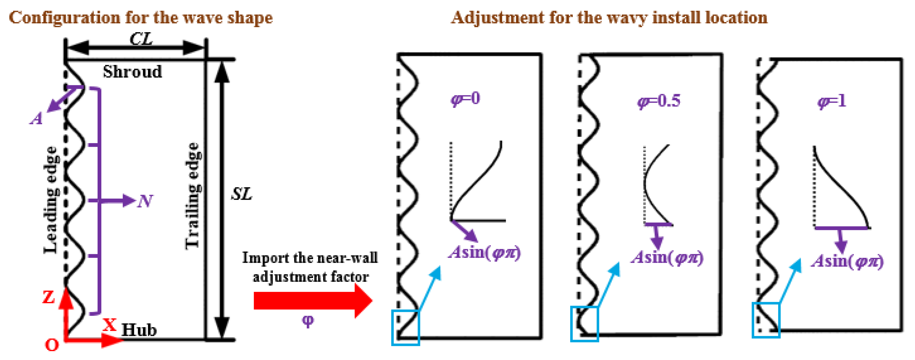
3.1. Parametric Approach

Bionic parameterization for the blade’s leading edge is mainly divided into two parts, namely, the configuration for the wave shape and the adjustment for the wavy install location. As presented in Figure 7, firstly, two parameters are introduced to determine the configuration for the wave shape, which are the wavenumber (n) and amplitude (A). After the configuration for the wave shape is determined, the near-wall adjustment factor (φ) is imported to adjust the wavy install location near the hub wall and shroud wall. Ultimately, three parameters are proposed to control the wave distribution at the leading edge of the blade.

A coordinate system is established in Figure 7, whose origin is the intersection of the leading edge line and the hub line, where X-axis is the chord direction and Y-axis is the span direction. Based on the coordinate system, the parametric process can be quantitatively described. To unite the forming process of the wave shape and the adjusting process of the wave location, a new parametric approach is defined as:

$$X=f(z)=-\frac{A}{2}\cos \left[\frac{2\pi N}{SL}(z-\frac{SL}{2N}\phi )\right]+\frac{A}{2}z\in [0,SL]$$

(10)

where A is the amplitude, φ is the near-wall adjustment factor, SL is the span length, n is the wavenumber.

3.2. Optimization Strategy

The optimization of the wavy leading edge established on the new parameter approach is then executed with a new optimization strategy. As presented in Figure 8, the optimization strategy consists of the Box-Behnken Design (BBD) sampling, the database generation, the optimization process, and the optimization results’ verification. In this part, the approach for each part will be introduced in detail.

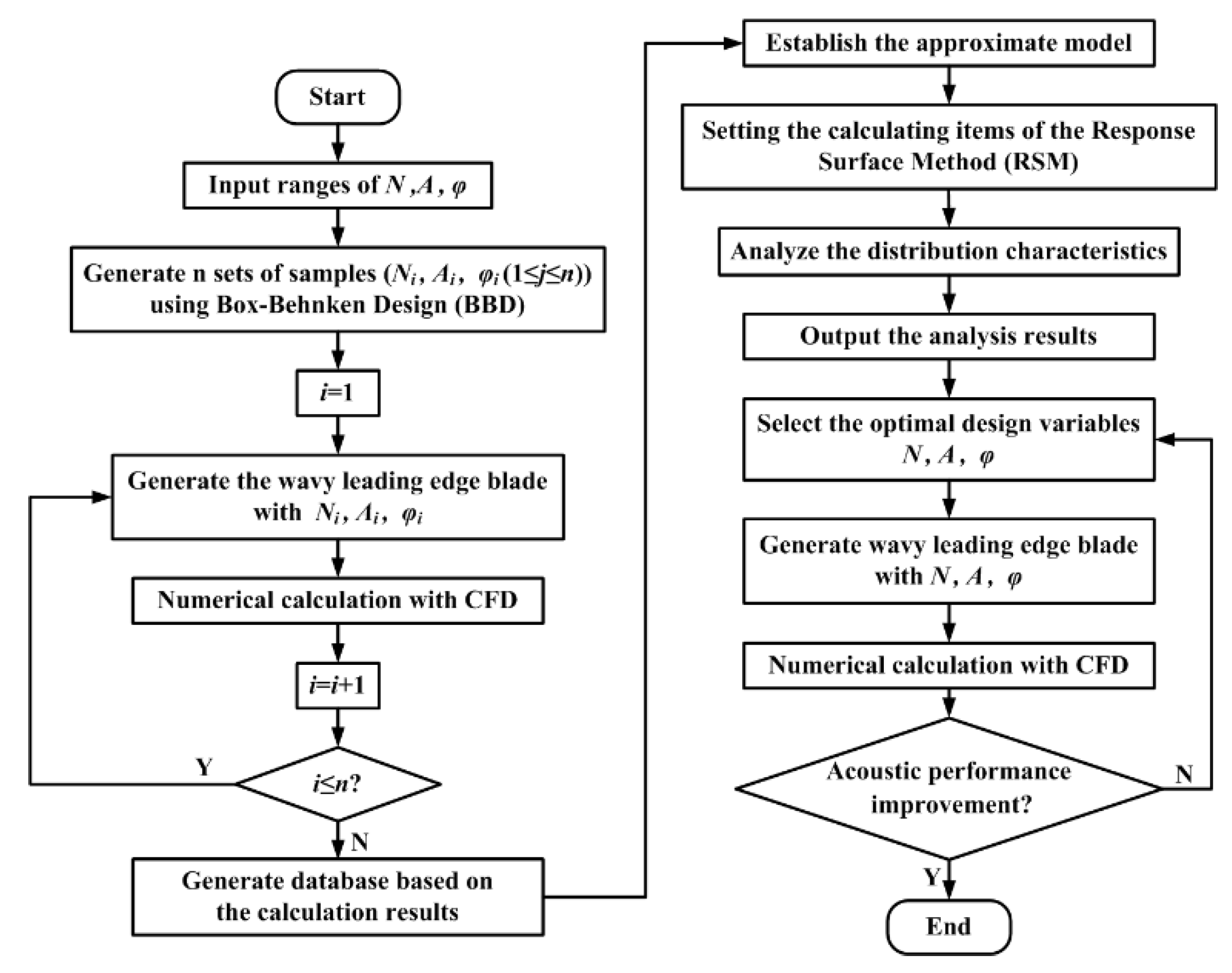
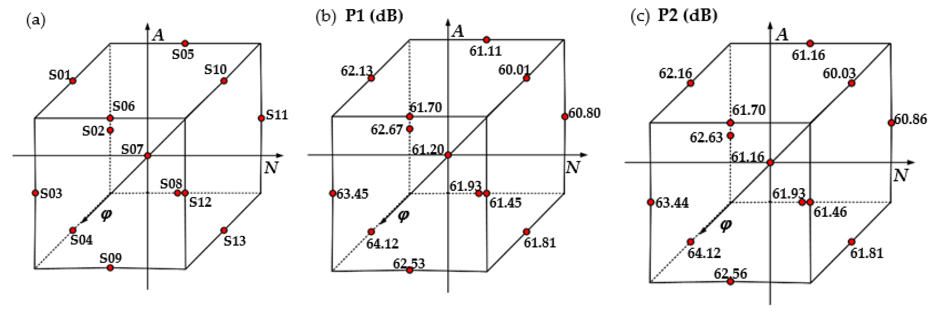
3.2.1. Box-Behnken Design (BBD) Sampling

As a Design of Experiment (DoE), BBD is a typical sampling methodology, which is applied in many fields [27,28]. Compared with the Central Composite Design (CCD) and the three-level full factorial designs, the number of experiments for the BBD is fewer [29]. Besides, the BBD does not contain extreme factor combinations; thus, they are avoided during sampling [30]. Hence, the sampling with BBD is utilized in this paper.

First, determine the ranges of variables (n, A, and φ). Considering the processing and manufacturing of the blade, the upper and lower limits of all design variables are listed in

Table 1. Ranges of variables.

Parameters	Values
Wave number (n)	[1,9]
Amplitude (A)	[1,13]
Near-wall adjustment factor (φ)	[0,1]

.

Then, code the design parameters according to the parameters ranges. The corresponding expressions and values are given in

Table 2. Design parameters and coded in BBD.

Items	Coded Variable Levels
	−1	0	1
	Xmin	(Xmax + Xmin)/2	Xmax
n	1	5	9
A	1	7	13
φ	0	0.5	1

. For the three factors, the number of experiments (Q) is 17, which can be defined as:

$$N=2k(k-1)+C_0$$

(11)

where k is the number of factors, k = 3 and C₀ is the number of central points, C₀ = 5.

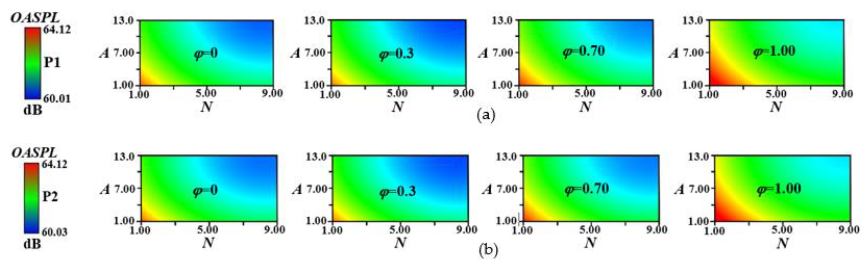
3.2.2. Database Generation

As shown in Figure 9a, the samples are generated based on the principle of three-factor BBD. Firstly, the bionic blade (attack angle α = 0°) for each sample is modeled via the parametric approach described in Section 3.1. Then, the sound fields are calculated with the simulation method mentioned in Section 2.2. According to Figure 4, the OASPL at the upper and lower surface of the NACA0018 blade is higher, so the corresponding monitoring points (P1 and P2) are defined as the target points. Finally, the calculation results of OASPL at the target points are shown in Figure 9b,c, and the database is generated.

3.2.3. Optimization Process

After the database is generated, an approximate model is established by learning the database, which can predict the relationship between the variables and the OASPL. Based on the application in acoustics [7,31], the Response Surface Method (RSM) is applied to predict the mathematical relationships, and the approximate model is simple and relatively accurate. Besides, the quadratic model is especially suitable for the three design parameters [32], which can be expressed as:

$${\widehat{y}}_i={\beta }_0+{\displaystyle \sum _{i=1}^3{\beta }_i^j{X}_i+}{\displaystyle \sum _{j=1}^3{\beta }_{ii}^j{(X_i)}^2+{\displaystyle \sum _{i\ne j}{\beta }_{ik}^j{X}_i{X}_k}}$$

(12)

where ${\widehat{y}}_i$ is the predicted value; $X_i$,$X_j$,$X_k$ are the design variables n, A, φ; ${\beta }_0$, ${\beta }_i^j$, ${\beta }_{ii}^j$,${\beta }_{ik}^j$ are the coefficients.

The formulas can be fitted by learning the database. Then the coefficient of determination (R²) is introduced [33] to verify the accuracy of the quadratic model. According to Figure 9, the values of R² for the fitting formulas are both 0.96 at the monitoring points (P1, P2), which meet the requirement that the value is greater than 0.8 [34]:

$$R^2=1-\frac{S{S}_{residual}}{S{S}_{tatal}}=1-\frac{{\displaystyle \sum _{i=1}^n{\left(y_i-{\widehat{y}}_i\right)}^2}}{{\displaystyle \sum _{i=1}^n{\left(y_i-\overline{y}\right)}^2}}$$

(13)

where $S{S}_{residual}$ is the sum of square of residuals; $S{S}_{total}$ is the total sum of squares; $y_i$, ${\widehat{y}}_i$, ${\overline{y}}_i$ are the actual value, the predicted value, and the mean value.

Based on the calculated quadratic model and the fitting process with RSM, the response surfaces are determined to predict the OASPL with different variables, which is given in Figure 10. As presented in Figure 10, due to the attack angle α = 0°, the overall OASPL distribution is the same at P1 and P2. It also can be seen that all three variables have an impact on the OASPL. The values of the OASPL have a decreasing trend with the increase in wavenumber (n) and amplitude (A), within the defined range. When the near-wall adjustment factor (φ) increases within the defined range, the values of the OASPL will first increase and then decrease.

Based on the response surface contours, optimal design variables are suggested, the values of which are n = 9, A = 13, φ = 0.3.

3.2.4. Optimization Results Verification

According to the suggested optimal parameters (n = 9, A = 13, φ = 0.3), the corresponding optimized bionic blade is modeled, which is shown in Figure 11a. The OASPL of the reference blade and the optimized bionic blade are simulated at the monitoring points in the Y-direction (Figure 4a). As shown in Figure 11b, compared with the reference blade, the optimized bionic blade can significantly reduce the OASPL, and the reduction is about 3 dB. Therefore, the proposed optimization strategy for the bionic blade is effective.

4. Results Analysis

For the original blade and the optimized blade, the aerodynamic performance and the acoustic performance is analyzed and the related mechanisms are discussed in this part.

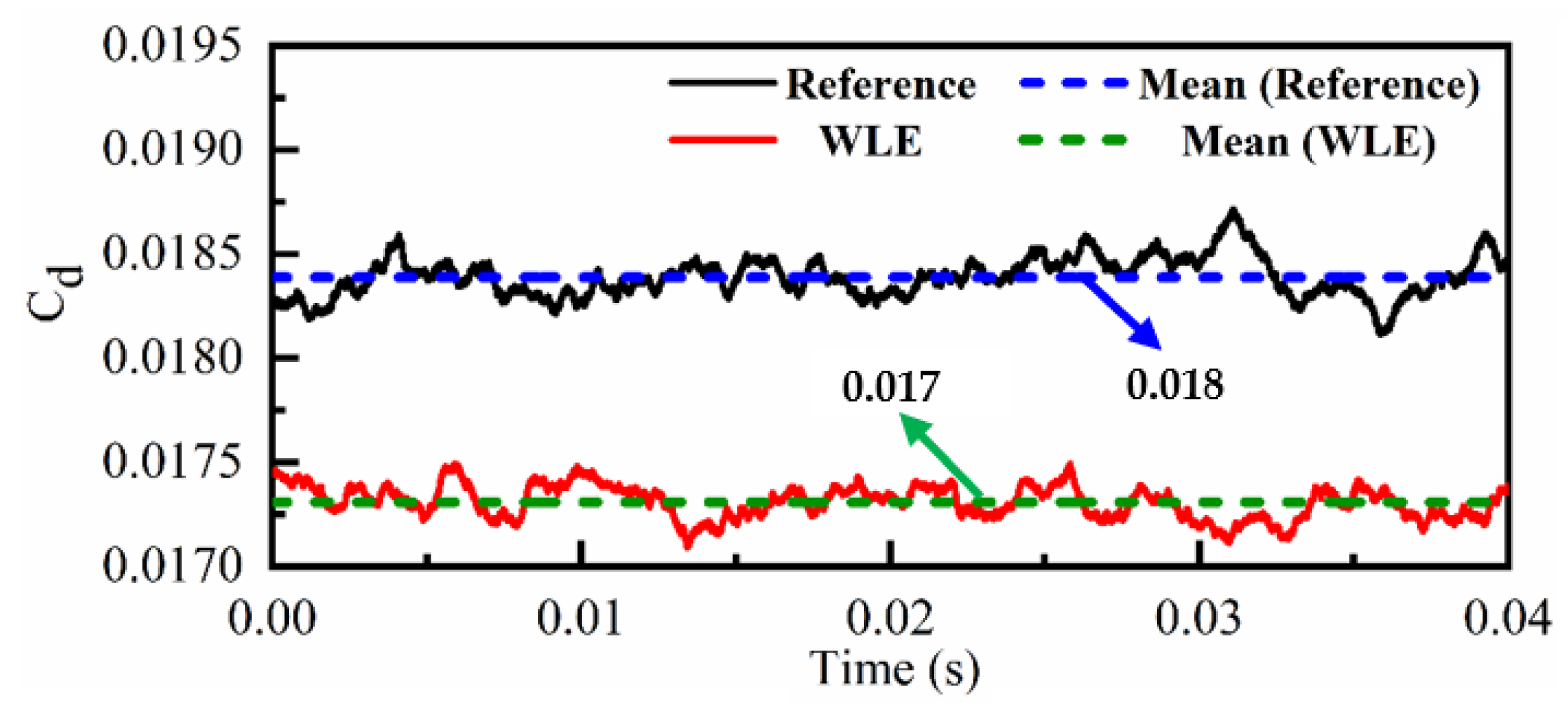
4.1. Aerodynamic Performance

For the optimized blade, three different span locations are extracted in Figure 12a, namely, peak, hill, and trough. According to Equation (8), the comparison of the time-averaged pressure coefficient distribution on the blade is given in Figure 12b. The WLE has an influence on the pressure coefficient distribution, which is mainly manifested in the upstream region. Compared with the original blade, the pressure coefficient shows a slow downward trend at peak and hill locations, which indicates the WLE can affect the flow field distribution of the upstream to some extent.

The blade drag coefficient is also a key performance, which can be defined as:

$$C_d=\frac{F_x}{0.5{\rho }_o{V}^{2}S}$$

(14)

where $F_x$ is the force on the blade in the X-direction; $V$ is the flow velocity relative to the blade; $S$ is the reference area, whose value is S = SL × CL.

The time history of the blade drag coefficient is shown in Figure 13. It can be found that the WLE can significantly reduce the drag coefficient. Then, the drag coefficient is processed by time average, and compared with the original blade, the mean drag coefficient of WLE is reduced by about 6%.

The magnitude of the wall shear stress can reflect the magnitude of the frictional drag, that is, one of the blade drag. Thus, the wall shear stress distributions of the blade for the original blade and optimized blade are presented in Figure 14. Compared with the original blade, the WLE can reduce the wall shear stress in the leading edge region, especially at peak and hill locations. The results further identify the drag reduction location and indicate that the WLE is effective for drag reduction.

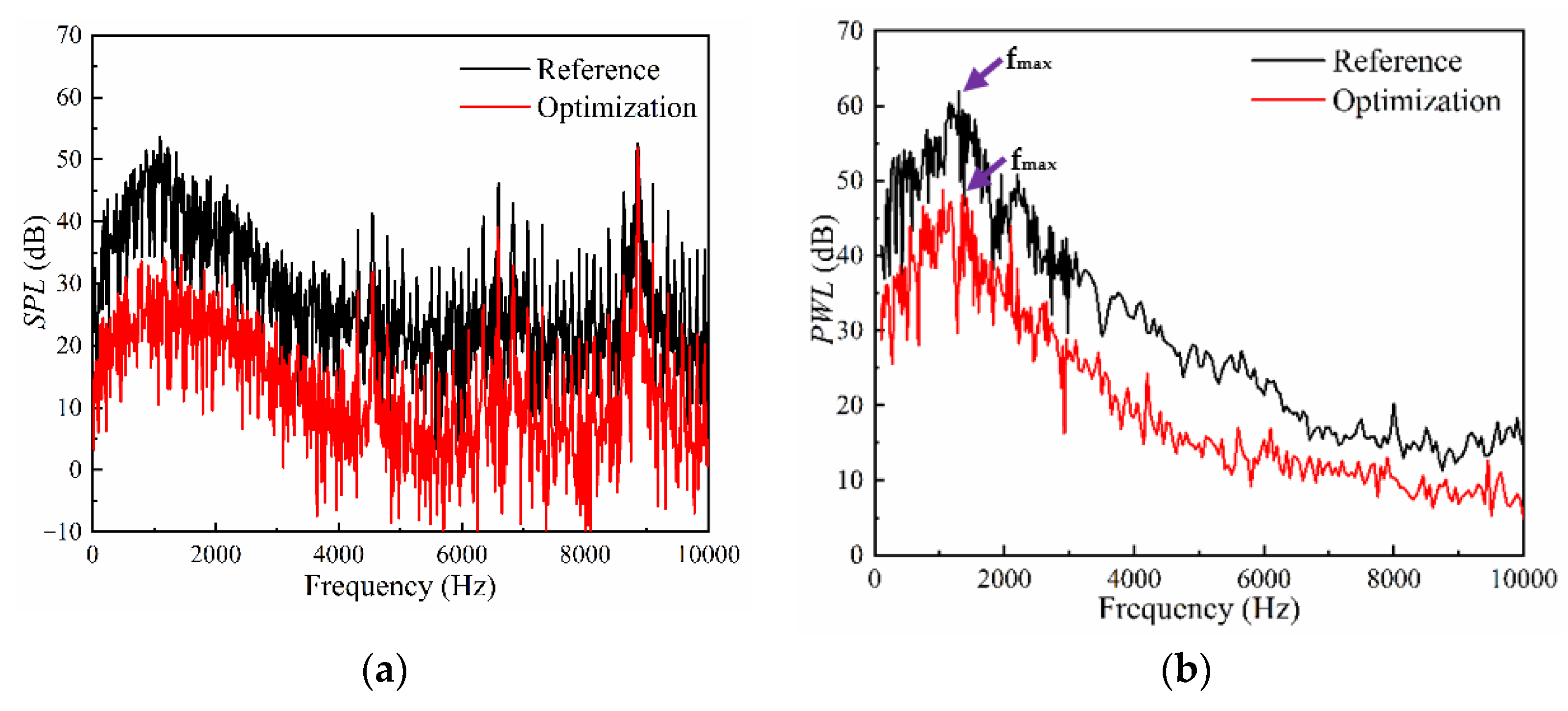
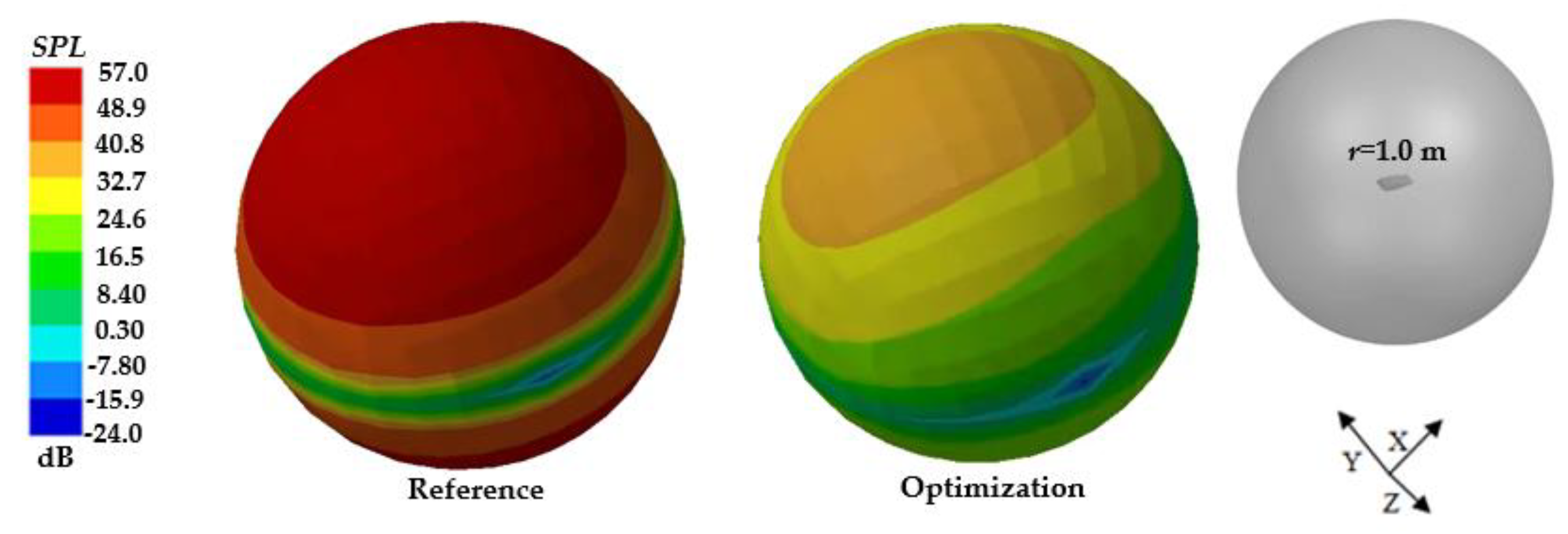
4.2. Acoustic Performance

For the acoustic performance, the comparisons of the acoustic spectrum between the original blade and the optimized blade are given in Figure 15. Figure 15a shows that the SPL at P1 is obviously reduced after optimization. Taking into account the randomness of monitoring point selection, the sound power level (PWL) is analyzed, the value of which is only determined by the sound source. As presented in Figure 15b, for the NACA blade, the maximum value of the PWL is at low-medium frequency, and the PWL of the optimized blade is smaller than that of the original blade.

$$PWL=10\lg \left(\frac{W}{W_{ref}}\right)$$

(15)

where W_ref is the reference sound power, whose value is 1 × 10⁻¹² W; W is the sound power.

To analyze the acoustic performance more intuitively, the blade is used as the sound source, and its influence on the spatial sound field distribution is given. A sphere centered at the blade’s centroid with a 1.0 m radius is established, and for each model, the spatial distribution of the maximum SPL is shown in Figure 16. It can be seen that the WLE can reduce the blade noise. Overall, the optimized blade has a beneficial effect on acoustic performance.

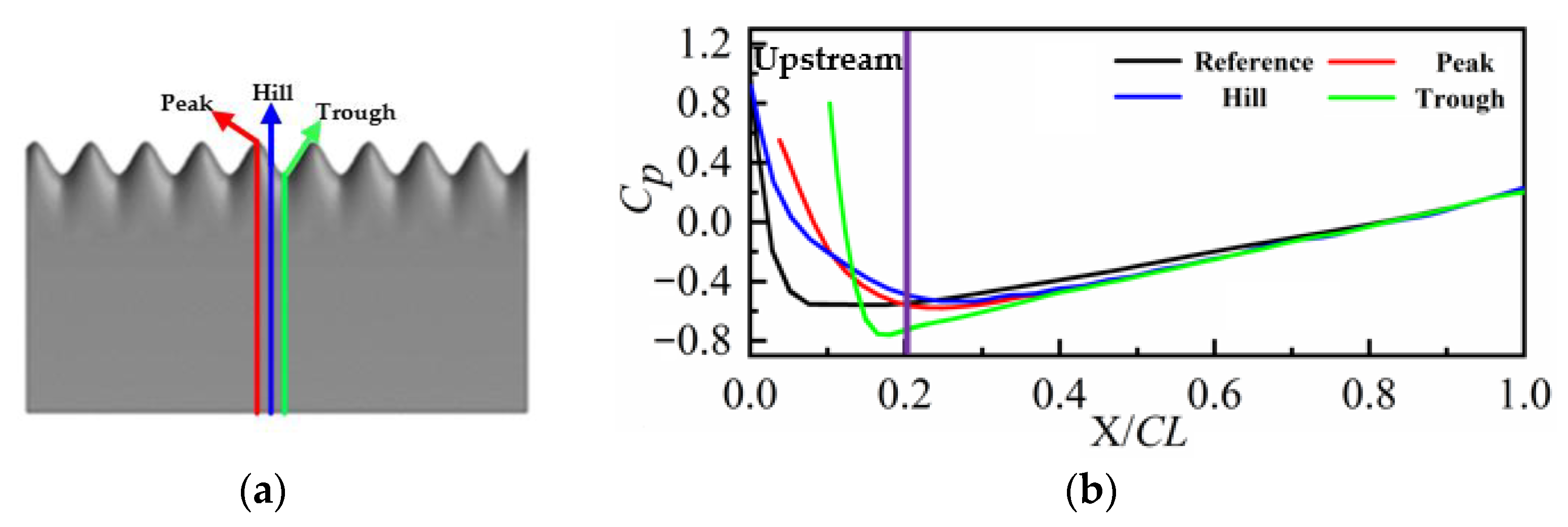
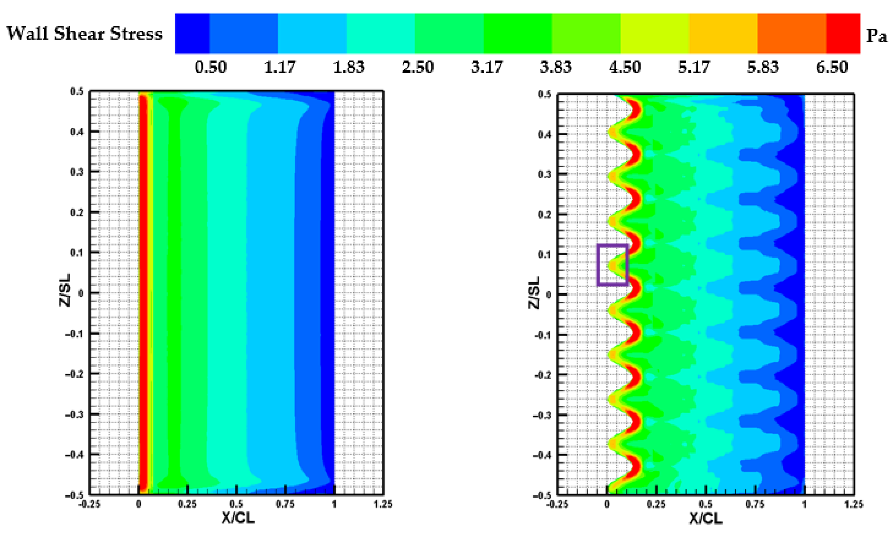
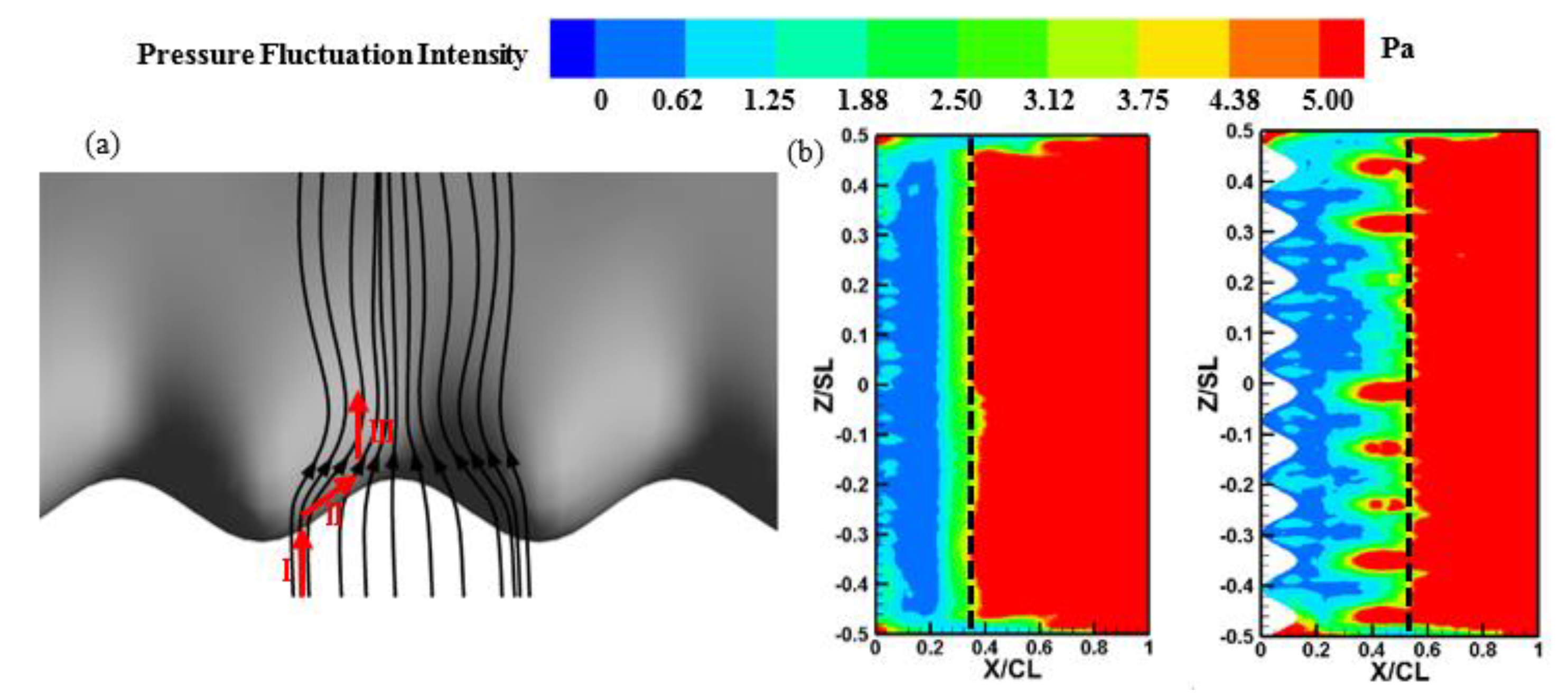
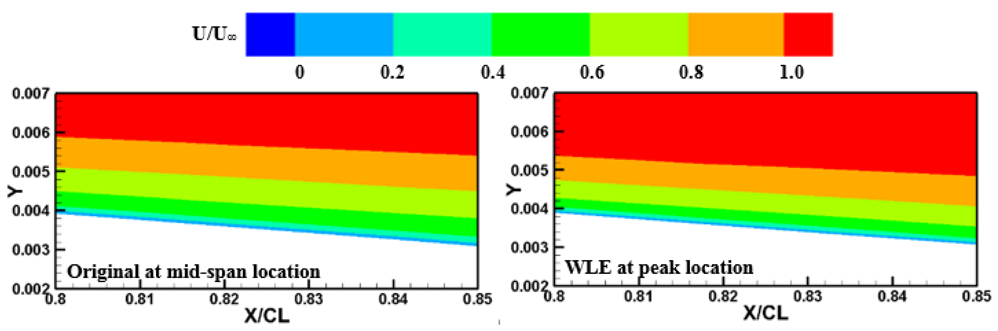
4.3. Mechanism Analysis

To further analyze the mechanism of drag reduction and noise reduction for the WLE blade, the streamlined distribution of WLE and the contour of the pressure fluctuation intensity are shown in Figure 17. The blade noise is related to the pressure fluctuation on the blade surface, so the pressure fluctuation intensity is introduced [35]:

$$\overline{P}(x,y,z)=\frac{1}{N}{\displaystyle \sum _{n=1}^N{P}_i}\left(x,y,z,\frac{n}{N}T\right)$$

(16)

$$P_f(x,y,z)=\sqrt{\frac{1}{N}{{\displaystyle \sum _{n=1}^N\left[P_i\left(x,y,z,\frac{n}{N}T\right)-\overline{P}\right]}}^2}$$

(17)

where $P_f$ is the pressure fluctuation intensity, $\overline{P}$ is the time-mean pressure, $P_i$ is the pressure at the netted nodes, T is the sampling time, n is the sampling quantity in the sample.

As shown in Figure 17a, the WLE structure can induce the spanwise velocity (II), which will reduce the impact of the incoming flow on the leading edge of the blade, especially at peak and hill locations. The spanwise velocity is not obvious at trough locations. Hence, the wall shear stress is reduced in the leading edge region (Figure 14), and the overall blade drag is reduced.

Figure 17b shows the comparison of pressure fluctuation intensity distribution on the blade surface, and it can be seen from the contours that the pressure fluctuation increases along the chord direction, which mainly is caused by the boundary layer separation at the trailing edge. Compared with the original blade, the high-pressure fluctuation zone of the WLE blade is significantly delayed in the downstream region (black dotted line).

The ratio of near-wall velocity and mainstream velocity in the downstream region is given in Figure 18. The boundary layer thickness of WLE at the peak location is thinner than that of the original at mid-span location. It is mainly due to the existence of spanwise velocity (II) at the wavy leading edge, which brings the air closer to the surface when it flows upstream of the WLE blade. Thus, the WLE blade can induce a further delay of the flow separation in the downstream region. That is the reason for the pressure fluctuation reduction and noise reduction.

5. Conclusions

To make up for the lack of aeroacoustic optimization of the bionic wavy leading edge in turbomachinery, a bionic optimization strategy about the leading edge of the typical blade is proposed. Using the NACA0018 blade as the basic blade, an optimal design scheme is obtained, which can improve the performance and reduce the noise.

The following conclusions can be gotten as:

• Based on the wavenumber and amplitude, a new parameter called the near-wall adjustment factor is proposed in this study to adjust the wavy leading edge of the closed impeller. A united parametric approach is then proposed, and it is proved that all parameters have an impact on the aerodynamic as well as acoustic performance.
• With the integration of the Box-Behnken Design (BBD) and other methods, an optimization strategy for the wavy leading edge of blade is established, and each process is introduced and evaluated. Ultimately, the optimal bionic blade is successfully obtained by the optimization strategy, which illustrates its effectiveness.
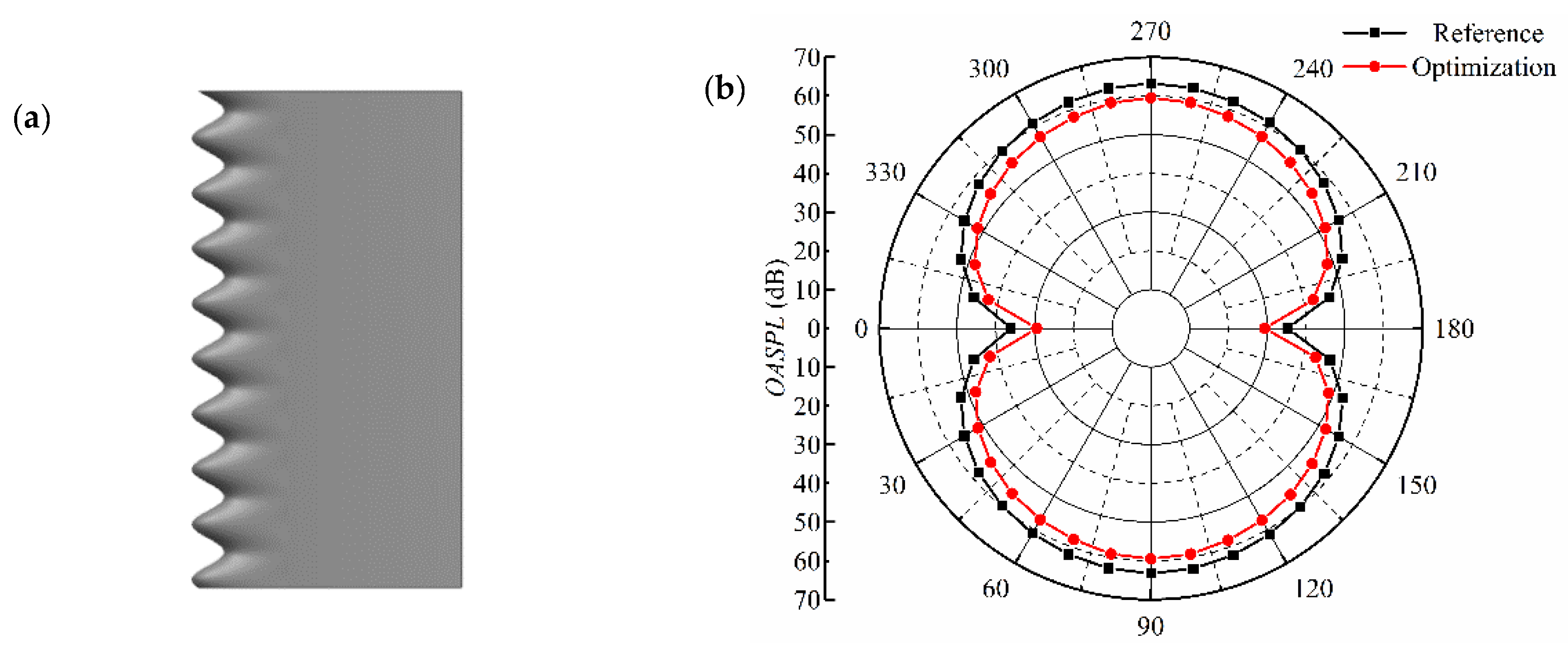
• The optimal wavy leading-edge blade is finally settled via optimization, and the corresponding external performance and inner flow mechanism is analyzed:
  • When compared to the original blade, the optimized blade can significantly reduce the blade’s drag, the mean drag coefficient of which has been reduced by about 6%;
  • According to the sound field results, it can be concluded that the optimized blade can reduce the noise, the OASPL of which can be reduced by as much as 3 dB.
• Through mechanism analysis, it can be found out that the wave structure can induce spanwise velocity at the leading edge, which causes a further delay in flow separation in the downstream region. Thus, both wall shear stress at the leading edge and the pressure fluctuation in the downstream region can be reduced. As a result, the drag and noise of the WLE blade are synchronously reduced.

References

1. Lu, Y.M.; Wang, X.F. Optimal design of the guide vane blade of the CAP1400 coolant pump based on the derived multi-source constrained zone. Nucl. Eng. Des. 2019, 342, 29–44. [Google Scholar] [CrossRef]
2. Yang, J.G.; Wang, R.; Zhang, M.; Liu, Y. Parametric study of rotor tip squealer geometry on the aerodynamic performance of a high subsonic axial compressor stage. J. Braz. Soc. Mech. Sci. 2021, 43, 1–13. [Google Scholar] [CrossRef]
3. Lu, Y.M.; Liu, H.R.; Wang, X.F.; Wang, H. Study of the operating characteristics for the high-speed water jet pump installed on the underwater vehicle with different cruising speeds. J. Mar. Sci. Eng. 2021, 9, 346. [Google Scholar] [CrossRef]
4. Sandra, V.S.; Rafael, B.T.; Juan, P.H.C.; Carlos, S.M. Experimental determination of the tonal noise sources in a centrifugal fan. J. Sound Vib. 2006, 295, 781–796. [Google Scholar] [CrossRef]
5. Carlo, C.; Davide, M. Numerical prediction of tonal noise in centrifugal blowers. In Proceedings of the Turbo Expo 2018, Oslo, Norway, 11–15 June 2018. [Google Scholar] [CrossRef]
6. Dong, X.; Dou, H.S. Effects of bionic volute tongue bioinspired by leading edge of owl wing and its installation angle on performance of multi-blade centrifugal fan. J. Appl. Fluid. Mech. 2021, 14, 1031–1043. [Google Scholar] [CrossRef]
7. Liu, H.R.; Lu, Y.M.; Li, Y.Y.; Wang, X.F. A bionic noise reduction strategy on the trailing edge of NACA0018 based on the central composite design method. Int. J. Aeroacoust. 2021, 20, 317–344. [Google Scholar] [CrossRef]
8. Song, X.P.; Wang, C.; Li, S.S.; Liu, H.P.; Zhang, C.H. Polyamide-poly (ionic liquid) reverse osmosis membrane with manifold excellent performance prepared via bionic capillary network for seawater desalinization. J. Membrane Sci. 2021, 632, 1–9. [Google Scholar] [CrossRef]
9. Graham, R.R. The silent flight of owls. J. Royal Aeronaut. Soc. 1934, 286, 837–843. [Google Scholar] [CrossRef]
10. Chen, W.J.; Qiao, W.Y.; Wei, Z.J. Aerodynamic performance and wake development of airfoils with wavy leading edges. Aerosp. Sci. Technol. 2020, 106, 1–27. [Google Scholar] [CrossRef]
11. Chen, W.J.; Qiao, W.Y.; Duan, W.H.; Wei, Z.J. Experimental study of airfoil instability noise with wavy leading edges. Appl. Acoust. 2021, 172, 1–8. [Google Scholar] [CrossRef]
12. Gao, H.T.; Zhu, W.C. Numerical investigation of bionic rudder with leading-edge protuberances. J. Offshore Mech. Arct. 2020, 142, 011802. [Google Scholar] [CrossRef]
13. Tong, F.; Qiao, W.Y.; Xu, K.B.; Wang, L.F.; Chen, W.J.; Wang, X.N. On the study of wavy leading-edge vanes to achieve low fan interaction noise. J. Sound Vib. 2018, 419, 200–226. [Google Scholar] [CrossRef]
14. Lyu, B.; Azarpeyvand, M. On the noise prediction for serrated leading edges. J. Fluid Mech. 2017, 826, 205–234. [Google Scholar] [CrossRef] [Green Version]
15. Nakhchi, M.E.; Naung, S.W.; Rahmati, M. High-resolution direct numerical simulations of flow structure and aerodynamic performance of wind turbine airfoil at wide range of Reynolds numbers. Energy 2021, 225, 120261. [Google Scholar] [CrossRef]
16. Shoukat, A.A.; Noon, A.A.; Anwar, M.; Ahmed, H.W. Blades optimization for maximum power output of vertical axis wind turbine. Int. J. Renew. Energ. Dev. 2021, 10, 585–595. [Google Scholar] [CrossRef]
17. Asadi, M.; Hassanzadeh, R. Effects of internal rotor parameters on the performance of a two bladed Darrieus-two bladed Savonius hybrid wind turbine. Energ. Convers. Manag. 2021, 238, 114109. [Google Scholar] [CrossRef]
18. Nakano, T.; Kim, H.J.; Lee, S.; Fujisawa, N.; Takagi, Y. A study on discrete frequency noise from a symmetrical airfoil in a uniform flow. In Proceedings of the JSME-KSME FEC5 Conference, Nagoya, Japan, 17–21 November 2002. [Google Scholar]
19. Fujisawa, N.; Shibuya, S.; Nashimoto, A.; Takano, T. Aerodynamic noise and flow visualization around two-dimensional airfoil. J. Vis. Jpn. 2001, 21, 123–129. [Google Scholar] [CrossRef] [Green Version]
20. Lu, Y.M.; Wang, X.F.; Liu, H.R.; Zhou, F.M.; Tang, T.; Lai, X.D. Analysis of the impeller’s tip clearance size on the operating characteristics of the underwater vehicle with a new high-speed water jet propulsion pump. Ocean Eng. 2021, 236, 109524. [Google Scholar] [CrossRef]
21. Lu, Y.M.; Wang, X.F.; Liu, H.R.; Li, Y.Y. Investigation of the effects of the impeller blades and vane blades on the CAP1400 nuclear coolant pump’s performances with a united optimal design technology. Prog. Nucl. Energ. 2020, 126, 103426. [Google Scholar] [CrossRef]
22. Ansys-Fluent Inc. Fluent User’s Guide; Ansys-Fluent Inc.: Pittsburgh, PA, USA, 2008. [Google Scholar]
23. Sagaut, P. Large Eddy Simulation for Incompressible Flows; Springer: Berlin/Heidelberg, Germany, 2006. [Google Scholar] [CrossRef]
24. Ffowcs Williams, J.F. Hydrodynamic noise. Annu. Rev. Fluid Mech. 1969, 1, 197–222. [Google Scholar] [CrossRef]
25. Kim, H.J.; Lee, S.; Fujisawa, N. Computation of unsteady flow and aerodynamic noise of NACA0018 airfoil using large-eddy simulation. Int. J. Heat Fluid Flow 2009, 27, 229–242. [Google Scholar] [CrossRef]
26. Mendonca, F.G.; Bonthu, S.K.; Kim, G. Transitional flow and aeroacoustic prediction of NACA0018 at Re=1.6×10⁵. In Proceedings of the Aiaa Theoretical Fluid Mechanics Conference, Atlanta, GA, USA, 16–20 June 2014. [Google Scholar]
27. Lee, S.H.; Kim, Y.J.; Lee, K.S.; Kim, S.J. Multiobjective optimization design of small-scale wind power generator with outer rotor based on Box–Behnken Design. IEEE. Trans. Appl. Supercon. 2016, 26, 1–5. [Google Scholar] [CrossRef]
28. Zhang, X.D.; Yu, S.M.; Gong, Y.; Li, Y.L. Optimization design for turbodrill blades based on response surface method. Adv. Mech. Eng. 2016, 8, 1–12. [Google Scholar] [CrossRef]
29. Ferreira, S.; Bruns, R.E.; Ferreira, H.S.; Matos, G.D.; David, J.M.; Brandao, G.C.; Silva, E.G.P.; Portugal, L.A.; Reis, P.S.; Souza, A.S.; et al. Box-Behnken design: An alternative for the optimization of analytical methods. Anal. Chim. Acta 2007, 597, 179–186. [Google Scholar] [CrossRef]
30. Rakic, T.; Kasagic-Vujanovic, I.; Jovanovic, M.; Jancic-Stojanovic, B.; Lvanovic, D. Comparison of full factorial design, Central Composite Design, and Box-Behnken Design in chromatographic method development for the determination of fluconazole and its impurities. Anal. Lett. 2014, 47, 1334–1347. [Google Scholar] [CrossRef]
31. Li, Z.; Su, X.P.; Tan, J.F.; Wang, H.N.; Wu, W.W. Multi-objective optimization of the layout of damping material for reducing the structure-borne noise of thin-walled structures. Thin Wall. Struct. 2019, 140, 331–341. [Google Scholar] [CrossRef]
32. Lu, Y.M.; Wang, X.F.; Wang, W.; Zhou, F.M. Application of the modified inverse design method in the optimization of the runner blade of a mixed-flow pump. Chin. J. Mech. Eng. 2018, 31, 127–143. [Google Scholar] [CrossRef] [Green Version]
33. Gunst, R.F. Response surface methodology: Process and product optimization using designed experiments. Technometrics 2008, 38, 284–286. [Google Scholar] [CrossRef]
34. Lim, J.W.; Beh, H.G.; Ling, D.; Ching, C.; Ho, Y.C.; Baloo, L.; Bashir, M.J.K.; Wee, S.K. Central Composite Design (CCD) applied for statistical optimization of glucose and sucrose binary carbon mixture in enhancing the denitrification process. Appl. Water Sci. 2016, 7, 3719–3727. [Google Scholar] [CrossRef] [Green Version]
35. Lu, Y.M.; Yang, J.G.; Wang, X.F.; Zhou, F.M. A symmetrical-nonuniform angular repartition strategy for the vane blades to improve the energy conversion ability of the coolant pump in the pressurized water reactor. Nucl. Eng. Des. 2018, 337, 245–260. [Google Scholar] [CrossRef]
Figure 1. Related pictures in introduction. (a) Wave structure; (b) Impeller form; (c) Pressure distribution.
Machines 09 00175 g001
Figure 2. Model and calculation domain. (a) NACA0018 blade; (b) Calculation domain.
Machines 09 00175 g002
Figure 3. Local mesh.
Machines 09 00175 g003
Figure 4. Mesh determination. (a) Monitoring points; (b) Mesh independence; (c) Y + value of the blade surface.
Machines 09 00175 g004
Figure 5. Comparison of the pressure distribution. (a) Experimental condition; (b) Time-averaged pressure coefficient.
Machines 09 00175 g005
Figure 6. Comparison of the sound field results. (a) Experimental condition; (b) Comparison of OASPL; (c) SPL spectrum.
Machines 09 00175 g006aMachines 09 00175 g006b
Figure 7. Wavy leading edge parameterization.
Machines 09 00175 g007
Figure 8. Flow chart of optimization strategy.
Machines 09 00175 g008
Figure 9. Distribution of the database on BBD. (a) BBD sampling; (b) OASPL at P1; (c) OASPL at P2.
Machines 09 00175 g009
Figure 10. Response surface contours. (a) P1; (b) P2.
Machines 09 00175 g010
Figure 11. Optimization results verification. (a) Optimized blade; (b) Comparison of the OASPL.
Machines 09 00175 g011
Figure 12. Comparison of the time-averaged pressure coefficient. (a) Chord position; (b) Time-averaged pressure coefficient.
Machines 09 00175 g012
Figure 13. Comparison of the drag coefficient.
Machines 09 00175 g013
Figure 14. Comparison of the wall shear stress.
Machines 09 00175 g014
Figure 15. Comparison of the frequency spectrum. (a) SPL spectrum; (b) PWL spectrum.
Machines 09 00175 g015
Figure 16. Comparison of the sound field distribution.
Machines 09 00175 g016
Figure 17. Streamlines and pressure fluctuation intensity. (a) Streamlines; (b) Pressure fluctuation intensity.
Machines 09 00175 g017
Figure 18. Comparison of the boundary layer thickness.
Machines 09 00175 g018