Design and Optimization of a Centrifugal Pump for Slurry Transport Using the Response Surface Method

Abstract

Since centrifugal pumps consume a mammoth amount of energy in various industrial applications, their design and optimization are highly relevant to saving maximum energy and increasing the system’s efficiency. In the current investigation, a centrifugal pump has been designed and optimized. The study has been carried out for the specific application of transportation of slurry at a flow rate of 120 m³/hr to a head of 20 m. For the optimization process, a multi-objective genetic algorithm (MOGA) and response surface methodology (RSM) have been employed. The process is based on the mean line design of the pump. It utilizes six geometric parameters as design variables, i.e., number of vanes, inlet beta shroud, exit beta shroud, hub inlet blade draft, Rake angle, and the impeller’s rotational speed. The objective functions employed are pump power, hydraulic efficiency, volumetric efficiency, and pump efficiency. In this reference, five different software packages, i.e., ANSYS Vista, ANSYS DesignModeler, response surface optimization software, and ANSYS CFX, were coupled to achieve the optimized design of the pump geometry. Characteristic maps were generated using simulations conducted for 45 points. Additionally, erosion rate was predicted using 3-D numerical simulations under various conditions. Finally, the transient behavior of the pump, being the highlight of the study, was evaluated. Results suggest that the maximum fluctuation in the local pressure and stresses on the cases correspond to a phase angle of 0°–30° of the casing that in turn corresponds to the maximum erosion rates in the region.

1. Introduction

Centrifugal pumps are being broadly used in coal, chemical, mining, and metallurgical industries mostly to transport solid–liquid mixtures referred to as slurries [1]. These pumps involve three-dimensional flows that are inherently turbulent and comprise secondary flows due to their complex internal passages [2]. Therefore, a good design for slurry transportation has always been a challenge, and several experimental and numerical studies to design and optimize centrifugal pumps can be found in the literature. George et al. performed a numerical study and provided a detailed analysis to minimize cavitation by improving the pump’s performance characteristics [3]. In another study [4], a detailed methodology for the inverse design method for a centrifugal impeller using the software HELIOX has been provided. Afterward, the authors also used numerical simulation to validate their results. Shojaeefard et al. [5] performed numerical studies to show the effects of specific geometric parameters on the pump impeller’s performance. They concluded that the passage width and blade outlet angle significantly affect the centrifugal pump’s performance. Kim et al. [6] performed a design optimization study for centrifugal pumps using numerical calculations. The authors proposed optimized geometry for the pump impeller and pump casing. Nourbakhsh et al. [7] compared the multi-objective particle swarm optimization method with the NSGA II algorithm to design and optimize the centrifugal pump. They tried to optimize variables ${\beta }_1^{hub}, {\beta }_1^{shr}$, and ${\beta }_2$. They consequently found important trade-offs in the optimum design of centrifugal pumps which they have proposed based on the Pareto front of two conflicting objective functions. Derakhshan et al. [8] optimized the impeller blade geometry using the artificial bee colony algorithm. They coupled three-dimensional Navier–Stokes optimization with the artificial bee colony algorithm to redesign the geometry and improve the performance of the barked 32–160 pump as a case study. They obtained 3.59% improvement in the efficiency and 6.89 m increase in the pressure head.

In the current study, a centrifugal pump impeller and casing geometry have been designed and optimized by coupling five different software packages, namely, ANSYS Vista CPD, response surface optimization software, DesignModeler, ANSYS TurboGrid, and ANSYS CFX. ANSYS Vista CPD obtains geometry based on required parameters using mean line calculations. The response surface optimization method was implemented to optimize the geometry obtained based on baseline calculations. More than one thousand design points were generated by varying geometrical parameters at the inlet and outlet of the impeller geometry. Three-dimensional geometries of impeller and casing were obtained using ANSYS DesignModeler software, and 3-D meshes of the geometries were generated in the software ANSYS TurboGrid. Finally, numerical simulations were carried out at different operating conditions to get the pump geometry’s characteristic maps. The pump geometry has been specifically optimized for the slurry transport of $120$m³ to a head of$20$ m in this study. After achieving the optimized geometry, complete characteristic maps were generated. Moreover, the erosion rate density of the designed pump geometry has been predicted using the Finnie model. Lastly, the pump’s transient behavior has been evaluated and reported in the current study, which has never been reported in the literature to the author’s best knowledge.

2. Initial Design of Pump and Pump Optimization

2.1. Pump and Volute Casing Design

The pump was designed using Vista CPD, which employs a 1-D approach for the centrifugal pump’s preliminary design in the current study. Assumptions and input parameters for the design are listed in

Table 1. Input parameter and assumptions.

Input Parameter	Symbol	Value
Volume flow rate	$Q \left[{\mathrm{m}}^3/\mathrm{hr}\right]$	$120$
Rotational speed	$N \left[\mathrm{RPM}\right]$	$1600$
Head rise	$H \left[\mathrm{m}\right]$	$20$
Inlet flow angle	${\theta }_1\left[\mathrm{degree}\right]$	${90}^{°}$
Hydraulic Efficiency	${\eta }_H$	$0.874$
Volumetric Efficiency	${\eta }_V$	$0.97$
Mechanical Efficiency	${\eta }_m$	$0.948$
Pump Efficiency	${\eta }_P$	$0.804$
Assumptions	Symbol	Value
Shaft min diameter factor	$D_f^{min}$	$1.1$
Hub to shaft diameter ratio	$\frac{D_{hub}}{D_{shaft}}$	$1.5$
Blade inlet angle at hub	${\beta }_1^{hub}\left[\mathrm{degree}\right]$	${27}^{°}$
Blade angle mean	${\beta }_1^{ML} \left[\mathrm{degree}\right]$	${19}^{°}$
Tip diameter	$D_{2t} \left[\mathrm{mm}\right]$	$280$
Blade angle at exit	${\beta }_2 \left[\mathrm{degree}\right]$	$22.5$

. The pump’s efficiency was calculated using built-in correlations in Vista CPD based on the past data for a given range of machine-specific speeds. Definitions of hydraulic efficiency, volumetric efficiency, mechanical efficiency, and pump efficiency are as follows.

2.1.1. Hydraulic Efficiency (${\eta }_H)$

Hydraulic efficiency is the most critical efficiency involved in the pump design that accounts for the head losses based on the hydrodynamic design, i.e., turning losses and friction losses, etc.

$${\eta }_H = \frac{H_i-H_{loss}}{H_i}$$

(1)

Here, $H_i$ is the ideal head, while losses based on hydrodynamic design are represented by$H_{loss}$.

2.1.2. Volumetric Efficiency $({\eta }_v)$

A certain amount of fluid $\left(Q_{leak}\right)$ from the main flow leaks from the tip clearance region to the eye of the pump. Volumetric efficiency in terms of the leaked flow $\left(Q_{leak}\right)$ and actual flow through the outlet $\left(Q\right)$ is thus given in the following equation.

$${\eta }_v=\frac{Q}{Q+Q_{leak}}$$

(2)

2.1.3. Mechanical Efficiency $\left({\eta }_v\right)$

Mechanical efficiency involves the losses due to mechanical friction and viscous friction, and it is defined below.

$${\eta }_v=\frac{P_{shaft}-P_{disk} }{P_{shaft}}$$

(3)

where $P_{shaft}$ is the power applied to drive the pump’s shaft and $P_{disk}$ is the power lost due to viscous and mechanical friction.

2.1.4. Pump Efficiency $\left({\eta }_p\right)$

Pump efficiency can be defined as in the equation given below.

$${\eta }_p ={\eta }_H\times {\eta }_V\times {\eta }_m$$

(4)

The shaft minimum diameter factor was calculated depending upon the maximum allowable shear stress of the shaft. The safety element is applied to the shaft minimum diameter, referred to here as the shaft minimum diameter factor, whereas the term $\frac{D_{hub}}{D_{shaft}}$ is the ratio of hub diameter to shaft diameter and taken as 1.5 in the current study.

2.1.5. Calculation of Leading Blade Angles

Leading-edge blade angles were computed using the Contingent method [9]. These angles were calculated relative to the shroud leading-edge blade angle as given below. It should be noted here that superscripts $hub$ and $shr$ correspond to the parameters related to hub and shrould of the rotor.

$${\beta }_1^{hub}={\tan }^{-1}\left(\frac{D_1^{shr}}{D_1^{hub}}{\tan }^{-1}\left({\beta }_1^{shr}\right)\right)$$

(5)

$${\beta }_1^{ML}={\tan }^{-1}\left(\frac{D_1^{shr}}{D_1^{ML}}{\tan }^{-1}\left({\beta }_1^{shr}\right)\right)$$

(6)

2.1.6. Calculations of Tip Diameter

Tip diameter is the diameter of the impeller at the mean line of the trailing edge. In this study, the tip diameter was computed by specifying the head coefficient $\left(\psi \right)$. Head coefficient could be defined as below.

$$\psi =\frac{g H}{U^2}$$

(7)

Blade angle at the trailing edge is an essential factor that defines the impeller width at the trailing edge $\left(b_2\right)$ because the flow rate at the outlet is a function of meridional velocity $\left(C_m\right)$ and cross-sectional area at the outlet$A_{out}$ as defined in the equation below. Impeller geometry computed by ANSYS Vista CPD is shown in Figure 1.

$$Q_{out}=C_m A_{out}$$

(8)

2.1.7. Specific Velocity

Pump efficiency will be maximum when the value of a specific speed $\left({\mathsf{\Omega }}_s\right)$ approaches 1. Specific speed $\left({\mathsf{\Omega }}_s\right)$ is defined in the equation below.

$${\mathsf{\Omega }}_s=\omega \frac{\sqrt{Q}}{g H}$$

(9)

Suction specific speed $\left({\mathsf{\Omega }}_{ss}\right)$ is a non-dimensional parameter that can be useful in the evaluation of pump cavitation performance. NPSH is the net positive suction head.

$$N_{sss}=\omega \frac{\sqrt{Q}}{{\left(g NPSH\right)}^{\frac{3}{4}}}$$

(10)

3. Pump Impeller Optimization

Pump geometry optimization was carried out using the RSM (response surface method) [10] coupled with a genetic algorithm (GA) [11]. Response surface methodology (RSM) is a tool used for optimization, regression analysis, and understanding the impact of design parameters on the objective function. It is well known and has been frequently adopted in the literature [12] based on its accuracy, trivial computational costs, and ease in implementation [13].

For the current study, the second-degree model of RSM has been adopted as given by Equation (11).

$$f\left(x\right)={\alpha }_0+{\displaystyle \sum }_{i=1}^n{\beta }_{i,i}{x}_i^2+{\displaystyle \sum }_{i=1}^{n-1}{\displaystyle \sum }_{j=i+1}^{nd}{\gamma }_{i,j}{x}_i{x}_j+{\displaystyle \sum }_{i=1}^n{\gamma }_i{x}_i$$

(11)

where $x_i$ and $f\left(x\right)$ denote variables and the system’s responses, respectively, while${\alpha }_0$, ${\beta }_{i,i}$,${\gamma }_{i,j}$, and ${\gamma }_i$ are regression coefficients. On the other hand, the term $n$ corresponds to the total number of design variables (e.g., for this study;$x_1\to x_6)$ as listed in

Table 2. Design variables used for the current work with their lower and upper bound limits.

Input Design Variable for the Optimization Procedure		Lower Bound	Upper Bound
Number of vanes (N)	$x_1$	$5$	8
Inlet beta shroud (${\beta }_1^{shr})$	$x_2$	$-5$	+5
Exit blade angle $({\beta }_2^M)$	$x_3$	${17.9}^{°}$	${23.1}^{°}$
Hub inlet draft	$x_4$	${27.1}^{°}$	${35}^{°}$
Rotation speed (rpm)	$x_5$	$1484$	1716
Rake angle	$x_6$	$-5^{°}$	$0^{°}$

. A list of the objective functions with respective constraints is given in

Table 3. Response variables and their constraints.

Response Variables	Constraints
Shaft power	Minimize
${\eta }_h$	Maximize
${\eta }_p$	Maximize
${\eta }_v$	Maximize

.

To develop the design of experiments (DOE) for the current work, a central composite design (CCD) option was utilized. The opted method of the design of the experiment, i.e., CCD, comprises an implanted factorial or fractional factorial design model with center points augmented with a group of “star points”. This method permits approximation of curvature [14] if required. If the distance from the center of the design space to a factorial point is ±1 unit for each factor, the distance from the center of the design space to a star point is|α| > 1. The exact value of α rests on defined properties anticipated for the design and the number of factors involved in the system. To uphold rotatability, the assessment of α is influenced by the number of experimental runs in the factorial design part of the CCD:

$$\alpha ={\left(2^n\right)}^{\frac{1}{4}}$$

Further details on the RSM and CCD can be found in the literature [10,13,14,15]. The list of design variables considered for the pump optimization problem with their upper and lower bounds is provided in Table 2. In contrast, the list of response variables is given in Table 3.

The various design combinations based on the selected design variables (Table 2) are based on the CCD are listed in

Table 4. Design of experiment using central composite design (CCD).

S. No.	$\mathit{N}\mathit{u}\mathit{m}\mathit{b}\mathit{e}\mathit{r} \mathit{o}\mathit{f}$ $\mathit{B}\mathit{l}\mathit{a}\mathit{d}\mathit{e}\mathit{s} \left(\mathit{N}\right)$	Inlet Beta Shroud $$\begin{gathered} ({\mathit{\beta }}_1^{\mathit{s}\mathit{h}\mathit{r}}) \\ \left(\mathbf{degree}\right) \end{gathered}$$	$$\begin{gathered} \mathbf{Exit} \mathbf{Blade} \mathbf{Angle} \\ ({\mathit{\beta }}_2^{\mathit{M}}) \\ \left(\mathbf{degree}\right) \end{gathered}$$	Hub Inlet Draft (degree)	$$\begin{gathered} \mathit{R}\mathit{a}\mathit{k}\mathit{e} \mathit{A}\mathit{n}\mathit{g}\mathit{l}\mathit{e} \\ \left(\mathbf{degree}\right) \end{gathered}$$	$\mathit{R}\mathit{P}\mathit{M}$
1	7	0.0	20.5	30.0	0.0	1600
2	5	0.0	20.5	30.0	0.0	1600
3	8	0.0	20.5	30.0	0.0	1600
4	7	−5.0	20.5	30.0	0.0	1600
5	7	5.0	20.5	30.0	0.0	1600
6	7	0.0	16.0	30.0	0.0	1600
7	7	0.0	25.0	30.0	0.0	1600
8	7	0.0	20.5	25.0	0.0	1600
9	7	0.0	20.5	35.0	0.0	1600
10	7	0.0	20.5	30.0	−5.0	1600
11	7	0.0	20.5	30.0	5.0	1600
12	7	0.0	20.5	30.0	0.0	1400
13	7	0.0	20.5	30.0	0.0	1800
14	6	−2.9	17.9	27.1	−2.9	1484
15	7	−2.9	17.9	27.1	−2.9	1716
16	6	2.9	17.9	27.1	−2.9	1716
17	7	2.9	17.9	27.1	−2.9	1484
18	6	−2.9	23.1	27.1	−2.9	1716
19	7	−2.9	23.1	27.1	−2.9	1484
20	6	2.9	23.1	27.1	−2.9	1484
21	7	2.9	23.1	27.1	−2.9	1716
22	6	−2.9	17.9	32.9	−2.9	1716
23	7	−2.9	17.9	32.9	−2.9	1484
24	6	2.9	17.9	32.9	−2.9	1484
25	7	2.9	17.9	32.9	−2.9	1716
26	6	−2.9	23.1	32.9	−2.9	1484
27	7	−2.9	23.1	32.9	−2.9	1716
28	6	2.9	23.1	32.9	−2.9	1716
29	7	2.9	23.1	32.9	−2.9	1484
30	6	−2.9	17.9	27.1	2.9	1716
31	7	−2.9	17.9	27.1	2.9	1484
32	6	2.9	17.9	27.1	2.9	1484
33	7	2.9	17.9	27.1	2.9	1716
34	6	−2.9	23.1	27.1	2.9	1484
35	7	−2.9	23.1	27.1	2.9	1716
36	6	2.9	23.1	27.1	2.9	1716
37	7	2.9	23.1	27.1	2.9	1484
38	6	−2.9	17.9	32.9	2.9	1484
39	7	−2.9	17.9	32.9	2.9	1716
40	6	2.9	17.9	32.9	2.9	1716
41	7	2.9	17.9	32.9	2.9	1484
42	6	−2.9	23.1	32.9	2.9	1716
43	7	−2.9	23.1	32.9	2.9	1484
44	6	2.9	23.1	32.9	2.9	1484
45	7	2.9	23.1	32.9	2.9	1716

. These designs were constructed and evaluated using Vista CPD. Computed results were later used to perform regression analysis by the response surface methodology. Details for input parameters, output parameters, and constraints are listed in

Table 5. Details for inlet and outlet parameters.

Input Parameters		Objective Functions
	Range	Parameters	Constraints
Number of vanes (N)	5–8	Shaft power	Minimize
Inlet beta shroud (${\beta }_1^{shr})$	−5–+5	${\eta }_h$	Maximize
$\mathrm{Exit} \mathrm{blade} \mathrm{angle} ({\beta }_2^M)$	${16}^{°}-{25}^{°}$	${\eta }_p$	Maximize
Hub inlet blade angle	${25}^{°}-{35}^{°}$	${\eta }_v$	Maximize
Rotation speed (rpm)	1200–1800
Hub inlet draft (degree)	${25}^{°}-{35}^{°}$

. Five input parameters with defined ranges were selected, i.e., number of vanes, inlet beta shroud, exit beta shroud, hub inlet blade angle, and the impeller’s rotational speed.

Multi-Objective Genetic Algorithm

The commonly implemented optimization algorithms in the literature are genetic algorithms [13,16,17,18,19,20,21] and particle swarm optimization (PSO) [22,23,24]. Both GA and PSO are iteration based and begin with a collection of initial data values and heuristic algorithms; however, the former utilizes discrete data and the latter works on the continuous data. It is registered in the published studies previously that both algorithms are extremely accurate; however, PSO presents comparatively better proficiency. At the same time, genetic algorithm (GA) is more valuable for constraint satisfaction challenges.

In light of the above discussion, the algorithm chosen for optimizing the current study is a multi-objective genetic algorithm (MOGA). Design variables mentioned above with their upper and lower limits have been displayed in Table 2. The solved regression model, i.e., solved Equation (11) for the RSM serves as an objective function for the MOGA. Previously conducted studies for the optimization of the pump have utilized complex and computationally expensive methods. Jiang et al. [25] utilized a CFD-DEM (computational fluid dynamics-discrete element method) approach for the fresh concrete pumping loss optimization. Ping et al. [26] utilized deep learning for the optimization of a multistage centrifugal pump. Similarly, Xiao and Tan [27] optimized pressure fluctuations for a multiphase flow in the pump. On the other hand, this is the first study, to the authors’ best knowledge, that utilizes response surface methodology coupled with 3D-RANS (Reynolds-averaged Navier–Stokes) simulations to compute the objective function that the MOGA would finally utilize to optimize the pump geometry.

Once the unknown coefficients of Equation (11) were found through RSM, it was used as an objective function for the multi-objective genetic algorithm (MOGA) [11]. For the current optimization process, Equation (11) was solved through RSM for shaft power, hydraulic efficiency, volumetric efficiency, and pump efficiency. For the optimization process, pump power was a constraint designated to be minimized, while hydraulic, volumetric, and pump efficiency were constraints to be maximized, as shown in Table 5. MOGA is based on the stochastic method and utilizes the principle of survival of the fittest [16]. The genetic algorithm is initialized through a random population of selected sizes based on the opted design variables that define the first generation. Every individual from the population is tested against the defined fitness function. In this process, each generation’s population gets improved through an iterative process using mutation, crossover, and elite selection. A schematic of the process is shown in Figure 2. Population size for the current study was selected as 100 combinations of the defined variables. The crossover fraction and mutation fraction values for the current problem were chosen as 0.9 and 0.01. A 10% elite of the total population was carried out as the next generation unchanged.

Figure 3 shows a variation of pump efficiency with rotational speed and hub draft angle. It can be observed that the effects of rotational speed on the pump efficiency are significant, but the hub draft angle has a minimum impact. It can also be noted that pump efficiency increases with the increase of the rotational speed, and then it starts decreasing after attaining a maximum value. A similar phenomenon was observed for all the hub inlet draft angles.

4. 3-D Computational Model

4.1. Governing Equations

On the other hand, Figure 4 shows a graph between shaft power, the blade angle beta, and the impeller’s rotational speed. It could also be depicted from Figure 4 that the count of vanes has a minimal impact on the power required to run the pump, and again, the shaft power varies significantly with the pump’s rotational speed. An increase in impeller rpm from 1400 to 1533 leads to a decrease in impeller power, but a further increase in rotational speed from 1533 to 1800 increases the pump’s required power.

Table 6. Parameters obtained for optimized impeller geometry.

Input Parameters		Objective Functions
Parameter	Value	Parameters	Value
Number of vanes (N)	7	Shaft power	9.06
Inlet beta shroud (${\beta }_1^{shr})$	1.7°	${\eta }_h$	97.5
$\mathrm{Exit} \mathrm{blade} \mathrm{angle} ({\beta }_2^M)$	22°	${\eta }_p$	89.3
Hub inlet blade angle	27°	${\eta }_v$	96.3
Rotation speed (rpm)	1533
Hub inlet draft (degree)	32°

shows the optimized parameter based on response surface optimization. A geometric comparison between base geometry and optimized geometry is shown in Figure 5.

In the previous section, an optimized model of the pump has been achieved based on the mean line 1-D computational model. Although 1-D calculations are robust, they are not as precise as 3-D calculations. Thus, this section provides a 3-D computational model to evaluate the performance of the optimized model accurately. Moreover, the design process has been conducted to design a pump specifically for slurry transport. Since the impact of slurry on the pump geometry, i.e., erosion and performance with slurry as a working fluid, could not be predicted using mean line design calculations, a 3-D computational model was necessary.

A steady form of the transport equations of continuity and momentum were solved for both phases (water and sand) using the Eulerian approach. Eulerian description of the equations is given in Equations (11)–(14) [28].

Continuity Equation for solid and fluid phase

$$\mathbf{\nabla }·\left({\alpha }_f{\rho }_f U_f\right)=0$$

(12)

$$\mathbf{\nabla }·\left({\alpha }_s{\rho }_s U_s\right)=0$$

(13)

Momentum Equation for solid and fluid phase

$$\mathbf{\nabla }·\left({\alpha }_f {\rho }_f{U}_f U_f \right)= -C_f \mathbf{\nabla }P+ \mathbf{\nabla }· ({\alpha }_f{\tau }_f)+ {\alpha }_f{\rho }_{f }g+ R+{\alpha }_f{\rho }_{f }\left(F_f+F_{l,f}+F_{v{m}_f}\right)$$

(14)

$$\mathbf{\nabla }·\left({\alpha }_s {\rho }_s{U}_s U_s \right)= -{\alpha }_s \mathbf{\nabla }P+ \mathbf{\nabla }· ({\alpha }_s{\tau }_s)+ {\alpha }_s{\rho }_{s }g+ R+{\alpha }_f{\rho }_{f }\left(F_f+F_{l,s}+F_{vm,s}\right)$$

(15)

In the above equation ${\alpha }_f and {\alpha }_s$ are the volume of fluid and solid while $U,\tau$ are velocity vector and shear stress tensor, respectively. Everywhere, subscript $f$and $s$ are used for fluid and solid, respectively. The term $p$ that appears in Equations (13) and (14) is an averaged pressure term and is the same for fluid and solid phases. It is presumed at the interface between the two phases [29].$F_l$ and $F_{vm,s}$ is the lift force and the virtual mass force per unit mass for either phase, respectively. $F_l,\mathit{s}$ is the lift force that could be calculated using the formula given by Equation (16) such that $F_l,\mathit{s}=-F_{l,f}$.

$$F_l,\mathit{s}=-0.5{\rho }_f{\alpha }_s\left({\mathit{V}}_{\mathit{f}}-{\mathit{V}}_{\mathit{s}}\right)\times \left(\mathbf{\nabla }·{\mathrm{V}}_{\mathrm{f}}\right)$$

(16)

Virtual mass effects come into play when the acceleration of the solid phase is observed in the fluid phase, and that results in a virtual mass force$F_{vm,s}$.

$$F_{vm,s}=0.5 {\alpha }_s{\rho }_f\left(\frac{d_f}{dt}\left( U_f\right)-\frac{d_s}{dt}\left(U_s\right)\right)$$

(17)

Coupling of solid with fluid could be either one-way or two-way coupling based on the value of the variable$\beta$. If the value of $\beta$ is less than 0.14, the one-way coupling is favored, while if it is more than or equal to 0.14, the two-way coupling is employed. Definition of $\beta$ is defined in the equation below.

$$\beta =\frac{{\alpha }_s{\rho }_s}{{\alpha }_f{\rho }_f}$$

(18)

The current study’s scope includes the wear prediction that occurs on the blade walls and the casing. The casing is likely to be more exposed to erosion than the blades, where higher tangential velocities tend to erode the casing.

Amongst available Reynolds-averaged Navier–Stokes (RANS) turbulence models, there exist two categories on the basis of how the boundary layer is treated in those models. In the first type of the RANS model, the boundary layer is not resolved, but a wall function is used to estimate the velocity profile, e.g., $k-ϵ$ turbulence model. The model uses two transport equations for the solution of turbulence kinetic intensity and dissipation. Simultaneously, turbulent viscosity is modeled as a product of turbulent velocity and turbulent length scale. The model is extremely computationally economical and efficient in resolving the turbulence in the mainstream flow. However, it does not solve the boundary but models it using wall functions. Therefore, it is not considered suitable for flows with boundary layer separation, flows with sudden changes in the mean strain rate, flows in rotating fluids, and flows over curved surfaces. On the other hand, the shear stress turbulence model combines two models [21,30,31,32], i.e., $k-\omega$ and $k-ϵ$ turbulence model according to the distance from the wall. Wilcox $k-\omega$ is utilized to resolve the flow in the vicinity of the walls for accurate prognostication of the boundary layer, whereas the $k-ϵ$ turbulence model is solving the flow in fully developed regions to gain advantage from its robustness, economy, and free stream independence [28,30]. Therefore, the shear stress turbulence model accounts for the transport of turbulent shear stress and avoids over-prediction of eddy viscosity. Numerous researchers [33,34,35,36,37,38] have adopted the shear stress transport (SST) turbulence model established by Menter [30] and achieved accurate aerodynamic predictions of rotating machines and complex flows. Based on the above discussion, the SST turbulence model is adopted for the current work as the flow is rotating. The accurate prediction of the boundary layer is critical for the precise evaluations of the erosion.

4.2. Erosion Model

Erosion initiates as particles collide against walls. This phenomenon is quite complicated and is a function of many parameters, such as multiphase effects, the effect of local cavities, properties of solid particles, shape, and size of particles, and local turbulent field. A simplified model suggested by Hutchings [39] shows that erosion rate density is modeled as a function of impact velocity and impact angle.

$$E= k{V}_p^n f\left(\gamma \right)$$

(19)

In the relation as mentioned above, $E$ characterizes a dimensionless mass, $V_p$ represents the velocity of the particle, and $f\left(\gamma \right)$ represents the impact angle in radians. The term $n$is assigned with different values for different metal ranges from 2.3 to 2.5. It is challenging to develop an erosion model that applies to a wide range of flow conditions and various geometrical features because tuning of model parameters always requires experimental data. Finnie [40] anticipated a model for ductile materials with a value of $n= 2$ that relates with the kinetic energy of the particles. Finnie’s model has been assumed to represent the wear in the current problem.

$$E= k{V}_p^2 f\left(\gamma \right)$$

(20)

$$\begin{array}{cc}f\left(\gamma \right)=\frac{1}{3}{\cos }^2\gamma \hfill & \hfill if\tan \gamma >\frac{1}{3}\\ f\left(\gamma \right)=\sin 2\gamma -3{\sin }^2\gamma \hfill & \hfill if\tan \gamma \le \frac{1}{3}\end{array}$$

(21)

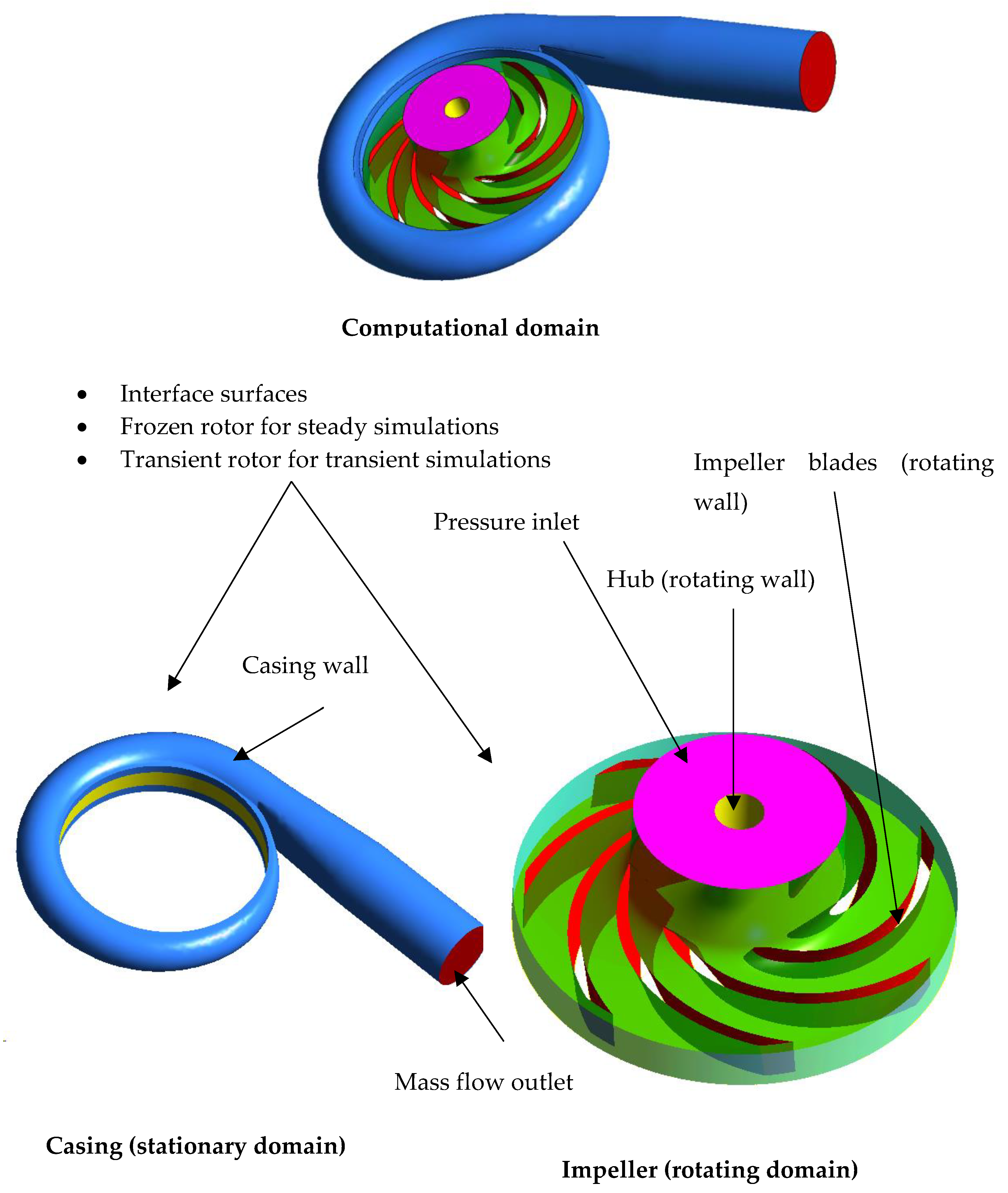
4.3. Computational Domain and Boundary Conditions

The current investigation, impeller, pump, and casing form the computational domain, as shown in Figure 6. Impeller geometry and the hub are modeled as a rotating domain that revolves at 1533 rpm, while the shroud is modeled as a stationary wall. On the other hand, the casing has been modeled as a stationary domain. The frozen rotor has been modeled as an interface between the impeller domain and casing domain for steady-state cases. In contrast, a transient stage interface type is implemented for unsteady simulations. At the inlet of the impeller, the total pressure boundary condition has been imposed, while the mass flow condition has been imposed on the outlet of the casing. Four different flow rates were used, i.e., $\frac{Q}{Q_{\eta \left(\max \right)}}=0.7, 0.8, 0.9,$and$1.0$. Here, $Q$ is the volume flow rate while $Q_{\eta \left(\max \right)}$ is the flow rate equivalent to the pump’s maximum efficiency, i.e., the point for which the rotor has been optimized. A volume concentration of 20% has been used for all the flow rates. Details of the simulations and particle distribution are listed in

Table 7. List of the simulations conducted for the current study.

Simulation Sets	Flow Rate $\frac{\mathit{Q}}{{\mathit{Q}}_{\mathit{\eta }\left(\mathit{m}\mathit{a}\mathit{x}\right)}}$	Analysis Type	Particle Distribution [micro]
			Min	Max	Ave	Std. dev.
1	0.7	Steady state	50	150	80	70
2	0.8		50	150	80	70
3	0.9		50	150	80	70
4	1.0		50	150	80	70
5	1.0	Unsteady Time step 0.001 s Simulation time 1.0 s Total number of time steps = 1000	50	150	80	70
Simulations to create characteristic curves
	$\frac{Q}{N_s}$	Simulations corresponding to various values of${\Omega }_s$	Particle Distribution [micro]
			Min	Max	Ave	Std. dev.
6	$1.0$	9 simulations	50	150	80	70
7	$0.1$	9 simulations	50	150	80	70
8	$0.01$	9 simulations	50	150	80	70
9	$0.001$	9 simulations	50	150	80	70
10	0.0001	9 simulations	50	150	80	70

. On this account, four sets of steady simulations were conducted with different flow rates.

For the unsteady simulation time step $\left(\mathsf{\Delta }t\right),$it was chosen equivalent to the time through which the rotor revolves through 1°. As mentioned above, the optimized value of the rotational speed of the rotor is 1533 rpm ($\omega =25.55 \mathrm{rad}/\mathrm{s}$); thus, time to complete $1^{°}= \mathsf{\Delta }t$= 0.11 ms. Meanwhile, $\mathsf{{\rm T}}$ can be referred to as time to complete one complete revolution ($\mathsf{{\rm T}}=\frac{2\mathsf{\Pi }}{\omega }=0.039 \mathrm{s})$. For the transient simulations, the total simulation time was chosen as 1.1 s, which corresponds to 10,000 time steps or 27.77 revolutions. It should be noted here that periodicity was achieved after ten revolutions; therefore, data of the first ten rotations was ignored.

It should be noted here that the Eulerian formulation has been used by providing individual densities of the solid phase and the liquid phase as opted by Adnan and Kim [41,42]. Although employing rheological models can improve the accuracy further, they are, however, not included in the current work to reduce the computational cost.

4.4. Mesh Generation

Structured mesh using hexahedral elements was generated for the impeller domain, while unstructured mesh was created for the stationary domain (volute casing). ANSYS TurboGrid was utilized to develop the structured mesh for the impeller domain with controlled topology. Meshes for the impeller domain and casing domain and the topology of the mesh are shown in Figure 7. The O-grid around the blade was constructed to capture the boundary layer accurately.

The value of $y^{+}$ was guaranteed to be less than 1 for both casing and impeller domains for all simulations to get maximum advantage to form the SST turbulence model [30].

The value $y^{+}$ is critical to get precise predictions for the SST turbulence model. Few turbulence models, such as the $k-ϵ$ turbulence model, do not solve the boundary layer but model it using the wall function. On the contrary, the SST turbulence model resolved the boundary layer, and it is essential to maintain $y^{+}<2$in the whole domain, and there must be fifteen nodes within the boundary layer, at least, for accurate predictions [30]. Consequently, it is ensured while generating the mesh that the value of $y_{max}^{+}<2$is everywhere in the domain. Further, the final mesh contains 27 elements within the boundary layer thickness.

The value of $y^{+}$ is dependent on the value of the $\mathsf{\Delta }y$ (distance of the first node from the wall), $D_H$ (hydraulic diameter), and Reynolds number $\left(Re\right)$. Equation (22) could be employed to estimate the value of the$\mathsf{\Delta }y$ that in turn will be used to compute the value of the $y^{+}$ [43].

$$\mathsf{\Delta }y=L y^{+}\sqrt{74} R{e}^{-\frac{13}{14}}$$

(22)

Four meshes were generated by varying different parameters listed in Table 1 to optimize the mesh for rotating and stationary domains.

For the mesh optimization, four different meshes were generated with parameters listed in

Table 8. Mesh details for mesh optimization study.

	Impeller Domain				Casing Domain	Number of Nodes	Memory Allocate [MB]	Computation Time for Ten Iteration	Computed Pump Power [kW]
Mesh	Number of Nodes in the Spanwise Direction	Number of Nodes in the O-Grid Region	Number of Nodes in the Tip Clearance Region	Number of Nodes in the Inlet Domain	Element Size in the Stationary Domain
M1	35	10	5	15	0.003	1,025,341	11,325	57	11.2
M2	45	20	7	20	0.002	1,523,452	18,256	97	10.7
M3	60	30	11	25	0.0015	2,742,863	35,261	195	9.26
M4	70	40	15	30	0.001	3,929,536	47,325	310	9.19

. The average corrosion rate was set as a parameter for optimization. Computed results for Mesh 3 and 4 matches closely; however, based on less computational power and time requirements, M3 was selected as the final mesh for all the simulations conducted for the current study.

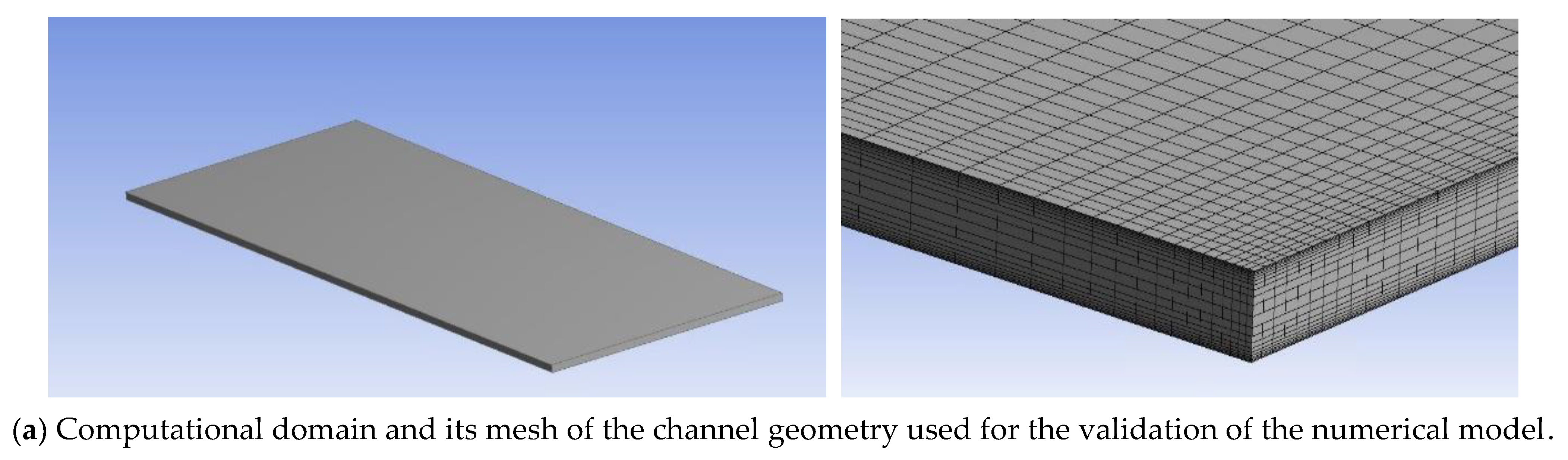
5. Validation of the Computational Model

Validation of the existing numerical model was completed by assessing the numerical model results utilized in the current study with the experimental research available in [44]. Experimental results introduced in [44] were acquired for a channel flow problem. Dimensions of the channel used were $6 \mathrm{m}\times 2 \mathrm{m}\times 0.05 \mathrm{m}.$ The geometrical model of the channel and mesh distribution is shown in Figure 3. Particles used for the study have an average diameter of $165 \mathsf{\mu }\mathrm{m}$ and density of $2680 \mathrm{kg}/{\mathrm{m}}^3$. The volume concentration of the particles at the inlet of the domain was $8.41\%$, while average velocity at the inlet of the domain of the fluid was $1.66 \mathrm{m}/\mathrm{s}$. The same geometry (Figure 8a) and other properties mentioned above used by [44] were implemented for the numerical model discussed above, and a comparison of the results is shown in Figure 8b,c. Figure 8b,c compare the concentration of particles and velocity profile for experimental results and results produced by the current numerical model. The comparison study shows that both works are in close agreement, and the present numerical model could predict erosion rate. The same validation procedure has been adopted in the literature as well by [29].

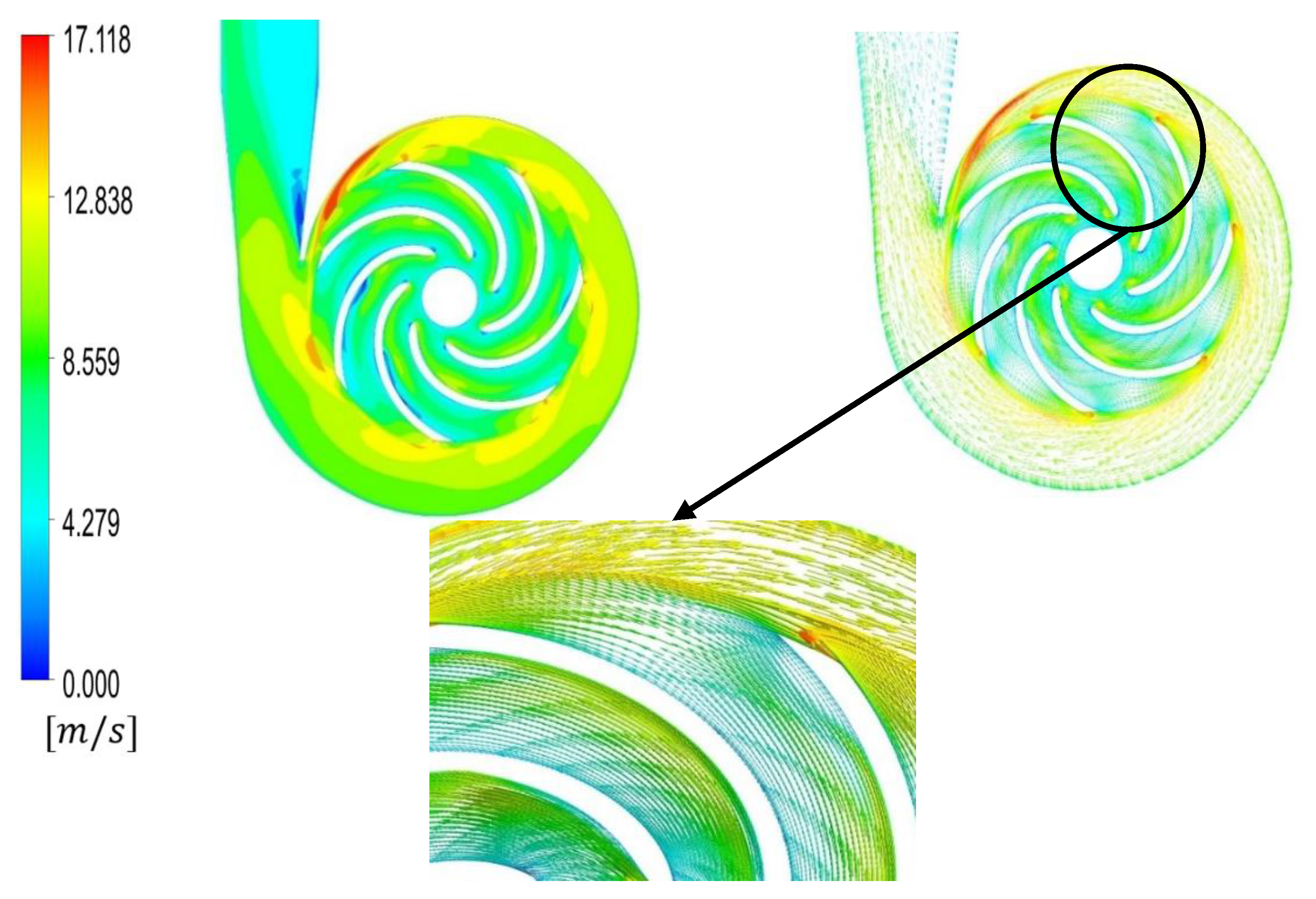
6. Computational Results

A centrifugal pump for slurry transport has been designed and optimized in the current study using mean line design calculations. To evaluate the optimized pump performance under slurry transport and to develop the characteristic maps of the pump, a 3-D computational model was developed and solved numerically using commercial software ANSYS CFX. Moreover, the pump’s transient behavior under slurry flow has been solved to predict the areas under the influence of the maximum erosion rate. Figure 9 and Figure 10 show the qualitative results of pressure, erosion rate, and velocity contours. Figure 9 shows pressure and erosion rate density contours on the walls of both rotating and stationary domains.

In contrast, Figure 10 shows contours and velocity vectors plotted on a turbo surface generated at the 50% span. It could be seen qualitatively in Figure 9 that erosion rate density is much higher at the casing than the erosion rates on the blades of the pump. It can be observed from velocity contours and vectors in Figure 10 that maximum velocity appears to be concentrated near the pump casing. In contrast, the velocities’ magnitudes are comparatively low in the flow region near the blades of the impeller. This is why higher erosion rate density can be observed in the casing region and not on the blades of the impeller.

6.1. Characteristic Maps of the Optimized Pump Geometry

Characteristic maps of the centrifugal pump were generated using 45 simulations at different values of $\frac{Q}{N_s}$ and specific speed$\left({\mathsf{\Omega }}_s\right)$. Five curves were plotted to complete the characteristic maps for the pump using values of $\frac{Q}{N_s}$ being 1.0, 0.1, 0.01, 0.001, and 0.001, where $Q$is the volume flow rate term and $N_s$ is the specific speed term. The relation between ${\mathsf{\Omega }}_s$ and $N_s$ is given in the equation below. Each curve was plotted using the results from nine simulations, as shown in Figure 11. It could be seen from Figure 11 that at specific speed values under 0.25, the efficiency of the pump is exceedingly small. Although, efficiency starts rising rapidly as specific speed rises above 0.25. As soon as specific speed approaches 0.5, efficiency increases faintly for a specific speed range from 0.5 to 1.0. Efficiency is maximum at a specific speed${ \mathsf{\Omega }}_s=1$ for all the curves. Moreover, for a specific speed range of 0.5 to 3.0, efficiency of the pump decreases for the curves at different values of $\frac{Q}{N_s}.$

6.2. Effect of Flow Rate on Erosion Rate Density

Figure 12 shows a variation of shear stress along the pump casing wall at various flow rates. Shear stress fluctuates twice at the throat of the casing near point C. It then keeps on increasing until point “D”, where it achieves maximum value. After that, it starts to decrease along with the casing at a steady rate. Variation of this shear stress depends on the local velocities and concentration of the sand particles. It can be seen from Figure 11 that wall shear stresses also vary with flow rates. Maximum shear stress was observed for a flow rate corresponding to maximum efficiency, i.e., $\frac{Q}{Q_{\eta \left(max\right)}}=1.0$ near point D. While minimum shear stress at point D was observed for a curve corresponding to$\frac{Q}{Q_{\eta \left(max\right)}}=0.7$. The difference between the maximum shear stress value and minimum stress value at point D was $32.68\%$. An interesting observation was made in this graph that shear stress values corresponding to $\frac{Q}{Q_{\eta \left(max\right)}}=1.0$ were higher in comparison with stress values at all other flow rates from point A to F. Afterwards, the amount of shear stress corresponding to $\frac{Q}{Q_{\eta \left(max\right)}}=1.0$ decreases suddenly and stays less from point F to H in comparison with stress values corresponding to all other flow rates.

Figure 13 shows a variation of erosion rate density along the casing wall from point A to J. Similar to the shear stress graph shown in Figure 12, erosion rate curves fluctuated near point C, but contrary to the previous graph, it dips down from point C to D. That increases marginally as it moves further. This is because erosion is a complex phenomenon that depends on many parameters, i.e., particle impact angle, particle size, particle velocity, concentration, etc., other than wall shear stress.

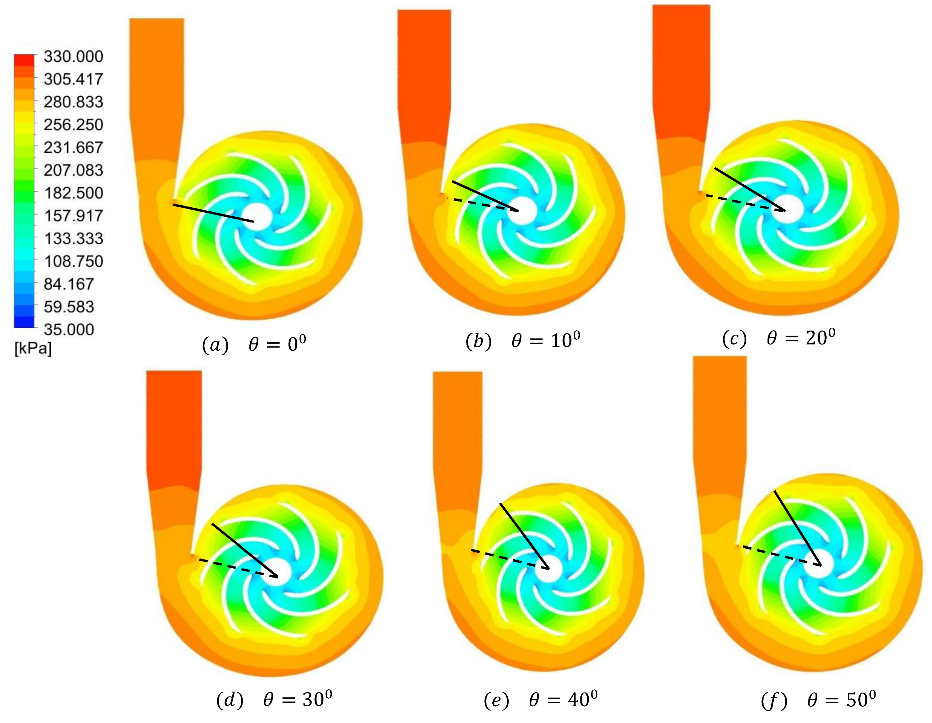
6.3. Transient Behavior of the Pump under a Slurry Flow Condition

This part of the results elaborates the variations in shear stress and pressure data during one rotor pitch rotation. The impeller of the pump consists of seven blades; thus, the elapsed angle corresponding to one pitch is $\frac{360°}{7}=51.42°\approx 50$. Furthermore, it is mentioned above that 1°of rotation corresponds to one time step ($\mathsf{\Delta }t=0.11 \mathrm{ms})$; therefore, one pitch will lapse nearly 51 time steps.

In the current study, result variations for one pitch are reported. Figure 14 shows pressure contours on the turbo surface extracted at 50% of the blade span corresponding to different phases, i.e., 0° − 50°. When the blade trailing edge is coincident with the line joining the throat of the casing to the axis of rotation, the blade phase angle is taken as $\theta =0^{°}$ as shown in Figure 14a. It can be seen that for phase angle $\theta =0^{°}-{30}^{°}$, maximum pressure at the casing exists then increases at some other locations, and it starts decreasing as the phase angle further increases from$\theta ={30}^{°}-{50}^{°}$. On the other hand, the variation of pressure along the casing is shown in Figure 15. Pressure increases clearly and significantly everywhere in the casing as the phase angle increases from $0^{°}-{30}^{°}$ and then it decreases from${30}^{°}-{50}^{°}$. The pressure curve in Figure 15 from point C to D shows a quite different distribution compared to all other curves plotted for various phase angles. A maximum difference of pressure was observed as 49.91%, just ahead of point C, between the forces recorded at a phase angle of $0^{°}$ and${30}^{°}$. This difference was recorded at 9.46% at the exit of the pump casing, reflecting that a fluctuating pressure will be recorded at the exit of the pump with a fluctuating frequency equal to the number of the pump’s impeller blades. The magnitude of flection for the current design was observed as 9.46%. Its dependence on other parameters, however, requires further investigations.

A variation of the wall shear stresses and the centrifugal pump’s casing at different phases of rotation is displayed in Figure 16. It can be seen that clearly there are three peaks of the wall shear stress—Peek 1 just ahead of C, Peak 2 and Peak 3 just after D. Location of Peak 1 and 2 are same for all phase angles; however, the location of Peak 3 changes slightly with the phase angle.

7. Conclusions

In the current study, design and optimization of the centrifugal pump geometry has been carried out to transport slurry with a flow rate of $120{ \mathrm{m}}^3{\mathrm{s}}^{-1}$to a given head of 20 m. Five different software packages were coupled to develop the optimization strategy. Optimized geometry was further investigated for performance prediction and erosion prediction under steady and transient conditions. The following points were concluded from the current study.

• Response surface optimization has proven to be an effective method for the optimization process in the ANSYS workbench environment, where it could be coupled with another meshing software and the Navier–Stokes solver.
• Pressure varies slightly, but shear stresses on the wall vary significantly with flow rate variations.
• Maximum pressure at the casing exits at phase angle θ = 0° − 30° and also increases at some other locations, and then it starts decreasing as the phase angle further increases from θ = 30° − 50°
• Fluctuating pressure was recorded at the pump’s exit with a fluctuating frequency equal to the number of impeller blades of the pump. The magnitude of fluctuation for the current design was observed as 9.46%. Its dependence on other parameters requires further investigation.

References

1. Wilson, K.C.; Addie, G.R.; Sellgren, A.; Clift, R. Slurry Transport Using Centrifugal Pumps; Gardners Books; Elsevier Applied Science: London, UK, 1992; ISBN 9781441935915. [Google Scholar]
2. Shah, S.R.; Jain, S.V.; Patel, R.N.; Lakhera, V.J. CFD for centrifugal pumps: A review of the state-of-the-art. Procedia Eng. 2013, 51, 715–720. [Google Scholar] [CrossRef] [Green Version]
3. George, A.; Muthu, D.P. CFD Analysis of Performance Characteristics of Centrifugal Pump Impeller to Minimizing Cavitation. In Proceedings of the International Conference on Current Research in Engineering Science and Technology (ICCREST-2016), Trichy, Tamilnadu, India, 4 May 2016; pp. 24–30. [Google Scholar]
4. Asuaje, M.; Bakir, F.; Kouidri, S.; Rey, R. Inverse Design Method for Centrifugal Impellers and Comparison with Numerical Simulation Tools. Int. J. Comut. Fluid Dyn. 2004, 18, 101–110. [Google Scholar] [CrossRef]
5. Shojaeefard, M.H.; Tahani, M.; Ehghaghi, M.B.; Fallahian, M.A.; Beglari, M. Numerical study of the effects of some geometric characteristics of a centrifugal pump impeller that pumps a viscous fluid. Comput. Fluids 2012, 60, 61–70. [Google Scholar] [CrossRef]
6. Kim, J.H.; Oh, K.T.; Pyun, K.B.; Kim, C.K.; Choi, Y.S.; Yoon, J.Y. Design optimization of a centrifugal pump impeller and volute using computational fluid dynamics. IOP Conf. Ser. Earth Environ. Sci. 2012, 15, 032025. [Google Scholar] [CrossRef]
7. Nourbakhsh, A.; Safikhani, H.; Derakhshan, S. The comparison of multi-objective particle swarm optimization and NSGA II algorithm: Applications in centrifugal pumps. Eng. Optim. 2011, 43, 1095–1113. [Google Scholar] [CrossRef]
8. Derakhshan, S.; Pourmahdavi, M.; Abdolahnejad, E.; Reihani, A.; Ojaghi, A. Numerical shape optimization of a centrifugal pump impeller using artificial bee colony algorithm. Comput. Fluids 2013, 81, 145–151. [Google Scholar] [CrossRef]
9. ANSYS 16.0 Vista RTD; Ansys Inc.: Canonsburg, PA, USA, 2016; Available online: https://www.ansys.com/products/fluids/ansys-vistatf (accessed on 26 June 2018).
10. ANSYS 16, Response Surface Optimization User Manual; Ansys Inc.: Canonsburg, PA, USA, 2016; Available online: https://www.ansys.com/products/platform/ansys-designxplorer (accessed on 12 August 2019).
11. Goldberg, D.E. Genetic Algorithms in Search, Optimization, and Machine Learning; Addison-Wesley Publishing Company, Inc.: Menlo Park, CA, USA, 1989; ISBN 0201157675. [Google Scholar]
12. Saeed, M.; Kim, M. Analysis of a recompression supercritical carbon dioxide power cycle with an integrated turbine design/optimization algorithm. Energy 2018, 165, 93–111. [Google Scholar] [CrossRef]
13. Saeed, M.; Kim, M.-H. Thermal-hydraulic analysis of sinusoidal fin-based printed circuit heat exchangers for supercritical CO2 Brayton cycle. Energy Convers. Manag. 2019, 193, 124–139. [Google Scholar] [CrossRef]
14. Saeed, M.; Khatoon, S.; Kim, M.-H. Design optimization and performance analysis of a supercritical carbon dioxide recompression Brayton cycle based on the detailed models of the cycle components. Energy Convers. Manag. 2019, 196, 242–260. [Google Scholar] [CrossRef]
15. Salim, M.S.; Saeed, M.; Kim, M.-H. Performance Analysis of the Supercritical Carbon Dioxide Re-compression Brayton Cycle. Appl. Sci. 2020, 10, 1129. [Google Scholar] [CrossRef] [Green Version]
16. Wang, K.; He, Y.-L. Thermodynamic analysis and optimization of a molten salt solar power tower integrated with a recompression supercritical CO2 Brayton cycle based on integrated modeling. Energy Convers. Manag. 2017, 135, 336–350. [Google Scholar] [CrossRef]
17. Li, H.; Su, W.; Cao, L.; Chang, F.; Xia, W.; Dai, Y. Preliminary conceptual design and thermodynamic comparative study on vapor absorption refrigeration cycles integrated with a supercritical CO2 power cycle. Energy Convers. Manag. 2018, 161, 162–171. [Google Scholar] [CrossRef]
18. Bahamonde Noriega, J.S. Design Method for s-CO2 Gas Turbine Power Plants Integration of Thermodynamic Analysis and Components Design for Advanced Applications, Report: P&E-2530; Delft University of Technology: Delft, The Netherlands, 2012. [Google Scholar]
19. Zhang, X.; Sun, X.; Christensen, R.N.; Anderson, M.; Carlson, M. Optimization of S-Shaped Fin Channels in a Printed Circuit Heat Exchanger for Supercritical CO2 Test Loop. In Proceedings of the 5th International Supercritical CO2 Power Cycles Symposium, San Antonio, TX, USA, 28–31 March 2016. [Google Scholar]
20. Shen, X.; Yang, H.; Chen, J.; Zhu, X.; Du, Z. Aerodynamic shape optimization of non-straight small wind turbine blades. Energy Convers. Manag. 2016, 119, 266–278. [Google Scholar] [CrossRef] [Green Version]
21. Ha, S.T.; Ngo, L.C.; Saeed, M.; Jeon, B.J.; Choi, H. A comparative study between partitioned and monolithic methods for the problems with 3D fluid-structure interaction of blood vessels. J. Mech. Sci. Technol. 2017, 31, 281–287. [Google Scholar] [CrossRef]
22. Venkata Rao, R.; Patel, V. Multi-objective optimization of combined Brayton and inverse Brayton cycles using advanced optimization algorithms. Eng. Optim. 2012, 44, 965–983. [Google Scholar] [CrossRef]
23. Xiao, D.; do Prado, J.C.; Qiao, W. Optimal joint demand and virtual bidding for a strategic retailer in the short-term electricity market. Electr. Power Syst. Res. 2021, 190, 106855. [Google Scholar] [CrossRef]
24. Zhang, H.; Liu, J.; Xiao, D.; Qiao, W. Security-Constrained Optimal Power Flow Solved with a Dynamic Multichain Particle Swarm Optimizer. In Proceedings of the 51st North American Power Symposium, NAPS 2019, Wichita, KS, USA, 13–15 October 2019. [Google Scholar]
25. Jiang, S.; Chen, X.; Cao, G.; Tan, Y.; Xiao, X.; Zhou, Y.; Liu, S.; Tong, Z.; Wu, Y. Optimization of fresh concrete pumping pressure loss with CFD-DEM approach. Constr. Build. Mater. 2021, 276, 122204. [Google Scholar] [CrossRef]
26. Ping, X.; Yang, F.; Zhang, H.; Zhang, J.; Zhang, W.; Song, G. Introducing machine learning and hybrid algorithm for prediction and optimization of multistage centrifugal pump in an ORC system. Energy 2021, 222, 120007. [Google Scholar] [CrossRef]
27. Xiao, W.; Tan, L. Design method of controllable velocity moment and optimization of pressure fluctuation suppression for a multiphase pump. Ocean Eng. 2021, 220, 108402. [Google Scholar] [CrossRef]
28. Versteeg, H.K.; Malalasekera, W. An Introduction to Computational Fluid Dynamics—The Finite Volume Method. In Fluid Flow Handbook; McGraw-Hill: Essex, UK, 1995; p. 267. [Google Scholar]
29. Pagalthivarthi, K.V.; Gupta, P.K.; Tyagi, V.; Ravi, M.R. CFD Predictions of Dense Slurry Flow in Centrifugal Pump Casings. World Acad. Sci. Eng. Technol. Int. J. Mech. Aerosp. Ind. Mechatron. Manuf. Eng. 2011, 5, 538–550. [Google Scholar]
30. Menter, F.R. Zonal two equation kappa-omega turbulence models for aerodynamic flows. In Proceedings of the 24th Fluid Dynamics Conference, Orlando, FL, USA, 6–9 July 1993. [Google Scholar]
31. Siddiqui, M.S.; Latif, S.T.M.; Saeed, M.; Rahman, M.; Badar, A.W.; Hasan, S.M. Reduced order model of offshore wind turbine wake by proper orthogonal decomposition. Int. J. Heat Fluid Flow 2020, 82, 108554. [Google Scholar] [CrossRef]
32. Saeed, M.; Berrouk, A.S.; Salman Siddiqui, M.; Ali Awais, A. Numerical investigation of thermal and hydraulic characteristics of sCO2-water printed circuit heat exchangers with zigzag channels. Energy Convers. Manag. 2020, 224, 113375. [Google Scholar] [CrossRef]
33. Cai, X.; Gu, R.; Pan, P.; Zhu, J. Unsteady aerodynamics simulation of a full-scale horizontal axis wind turbine using CFD methodology. Energy Convers. Manag. 2016, 112, 146–156. [Google Scholar] [CrossRef]
34. Sayed, M.A.; Kandil, H.A.; Shaltot, A. Aerodynamic analysis of different wind-turbine-blade profiles using finite-volume method. Energy Convers. Manag. 2012, 64, 541–550. [Google Scholar] [CrossRef]
35. Sörensen, N.N.; Michelsen, J.A.; Schreck, S. Navier-Stokes predictions of the NREL phase VI rotor in the NASA Ames 80 ft × 120 ft wind tunnel. Wind Energy 2002, 5, 151–169. [Google Scholar] [CrossRef]
36. Saeed, M.; Kim, M.-H. Thermal and hydraulic performance of SCO2 PCHE with different fin configurations. Appl. Therm. Eng. 2017, 127, 975–985. [Google Scholar] [CrossRef]
37. Saeed, M.; Kim, M.-H. Aerodynamic performance analysis of an airborne wind turbine system with NREL Phase IV rotor. Energy Convers. Manag. 2017, 134, 278–289. [Google Scholar] [CrossRef]
38. Saeed, M.; Kim, M.-H. Airborne wind turbine shell behavior prediction under various wind conditions using strongly coupled fluid structure interaction formulation. Energy Convers. Manag. 2016, 120, 217–228. [Google Scholar] [CrossRef]
39. Hutchings, I. Mechanical and metallurgical aspects of the erosion of metals. Wear 1979, 393–427. [Google Scholar]
40. Finnie, I. Some observations on the erosion of ductile metals. Wear 1972, 19, 81–90. [Google Scholar] [CrossRef]
41. Aslam Noon, A.; Kim, M.H. Erosion wear on Francis turbine components due to sediment flow. Wear 2017, 378–379, 126–135. [Google Scholar] [CrossRef]
42. Noon, A.A.; Kim, M.H. Erosion wear on centrifugal pump casing due to slurry flow. Wear 2016, 364–365, 103–111. [Google Scholar] [CrossRef]
43. ANSYS CFX CFX-Pre User’s Guide Release 16.0. 2015. Available online: https://www.ansys.com/products/fluids/ansys-cfx (accessed on 25 November 2019).
44. Roco, C.; Addie, G.R. Analytical Model and Experimental studies on Slurry flow and erosion in pump casings. Slurry Transp. 1983, 8, 263–275. [Google Scholar]
Figure 1. Initial impeller geometry generated using ANSYS Vista CPD.
Machines 09 00060 g001
Figure 2. Schematic genetic algorithm.
Machines 09 00060 g002
Figure 3. Variation of pump efficiency with rotational speed and hub inlet draft angle.
Machines 09 00060 g003
Figure 4. Variation of pump power with rotational speed and blade angle beta.
Machines 09 00060 g004
Figure 5. Comparison between base geometry and optimized geometry.
Machines 09 00060 g005
Figure 6. Computational domain and boundary conditions.
Machines 09 00060 g006
Figure 7. Mesh for the impeller and volute casing.
Machines 09 00060 g007
Figure 8. Validation of the computational model.
Machines 09 00060 g008aMachines 09 00060 g008b
Figure 9. Pressure and erosion rate density contours on the walls of the impeller and casing walls.
Machines 09 00060 g009
Figure 10. Velocity contours and velocity vector on a plane at 50% span location.
Machines 09 00060 g010
Figure 11. Characteristic curves of the centrifugal pump.
Machines 09 00060 g011
Figure 12. Variation of wall shear stress along the walls of the pump casing at different flow rates.
Machines 09 00060 g012
Figure 13. Variation of erosion rate density along the walls of casing with corresponding flow rates.
Machines 09 00060 g013
Figure 14. Pressure contours plotted on the turbo surface at 50% of the span corresponding to various phase angles.
Machines 09 00060 g014
Figure 15. Variation of the pressure along with the casing of the centrifugal pump at different phases of rotation.
Machines 09 00060 g015
Figure 16. Variation of the wall shear stresses along the casing of the centrifugal pump at different phases of rotation.
Machines 09 00060 g016