Article

Valve Deadzone/Backlash Compensation for Lifting Motion Control of Hydraulic Manipulators

1
School of Aerospace Engineering, Beijing Institute of Technology, Beijing 100081, China
2
School of Mechanical Engineering, Nanjing University of Science and Technology, Nanjing 210094, China
*
Author to whom correspondence should be addressed.
Machines 2021, 9(3), 57; https://doi.org/10.3390/machines9030057
Submission received: 13 February 2021 / Revised: 1 March 2021 / Accepted: 2 March 2021 / Published: 8 March 2021
(This article belongs to the Special Issue Advanced Control of Industrial Electro-Hydraulic Systems)

Abstract

:
In this paper, a novel nonlinear model and high-precision lifting motion control method of a hydraulic manipulator driven by a proportional valve are presented, with consideration of severe system nonlinearities, various uncertainties as well as valve backlash/deadzone input nonlinearities. To accomplish this mission, based on the independent valve orifice throttling process, a new comprehensive pressure-flow model is proposed to uniformly indicate both the backlash and deadzone effects on the flow characteristics. Furthermore, in the manipulator lifting dynamics, considering mechanism nonlinearity and utilizing a smooth LuGre friction model to describe the friction dynamics, a nonlinear state-space mathematical model of hydraulic manipulation system is then established. To suppress the adverse effects of severe nonlinearities and uncertainties in the system, a high precision adaptive robust control method is proposed via backstepping, in which a projection-type adaptive law in combination with a robust feedback term is conducted to attenuate various uncertainties and disturbances. Lyapunov stability analysis demonstrates that the proposed control scheme can acquire transient and steady-state close-loop stability, and the excellent tracking performance of the designed control law is verified by comparative simulation results.

1. Introduction

Hydraulic systems have been extensively applied in heavy manipulators [1,2,3,4] due to their good capabilities, such as high power/weight ratio, large output force, etc., especially in the operation of load-lifting with heavy load gravity. However, the control of electro-hydraulic systems is very challenging because the hydraulic system involves not only severe nonlinearities, such as mechanism nonlinearity, flow nonlinearity and friction nonlinearity, but also various modeling uncertainties (i.e., parametric uncertainties and uncertain nonlinearities). Thus, the traditional linear control methods have become more and more difficult to satisfy the demand of modern hydraulic systems. To cope with these issues, dozens of advanced nonlinear controllers have been proposed, such as feedback linearization control [5,6,7], nonlinear adaptive control [8,9,10] and adaptive robust control [11,12,13].
In most hydraulic control applications, nozzle-flapper-based servovalves are utilized as the control elements by virtue of fast response and high precision. Although servovalves have good controllability, their own defects are also obvious, that is, they are expensive and prone to malfunction due to fluid contamination. As a result, the electro-hydraulic systems controlled by servovalves have low reliability and poor economy. In recent decades, the proportional servo technology, using proportional valves as the control elements, has developed rapidly and received widespread attention in industrial fields. Compared to servovalves, proportional valves possess various advantages. They are much cheaper and have higher reliability because less accuracy is required in the manufacturing of spool and valve sleeve, and vulnerable nozzle-flapper structure is replaced by proportional elements. The electric feedback form is also employed in proportional valves to construct their internal closed-loop control, so they are less sensitive to oil contamination and simultaneously retain satisfactory servo control performance. Thereby, they are more suitable for industrial environments.
However, because of less precise manufacturing accuracy, proportional valves usually encounter backlash/deadzone input nonlinearities existing between the valve spool and the valve sleeve, which are one of the most typical features different from servovalves. Generally, the process of manufacturing proportional valves can be divided into two modes, namely, the backlash mode and the deadzone mode. In the backlash mode, there is a backlash between the valve spool and the valve sleeve, which may raise stability concerns due to the increased flow gain near neutral spool position. The deadzone mode, meaning that there exists overlapped part between the valve spool and the valve sleeve, may result in response to lag because a small control input cannot drive the spool in neutral spool position. Practice reveals that the existence of a backlash/deadzone may lead to reduced control performance, even instability. Furthermore, valve backlash/deadzone input nonlinearities, coupled with other system nonlinearities and various uncertainties, make it harder to control the hydraulic systems controlled by proportional valves. Thus, how to effectively compensate the influence of valve backlash/deadzone input nonlinearities in the presence of severe nonlinearities and modeling uncertainties has always been a practically important problem.
Regretfully, there are few works considering valve backlash nonlinearities, so the following discussion mainly focuses on the existing control method of valve deadzone compensation. As pointed out in [14], there are generally two kinds of methods to alleviate the effects of deadzone in the literature. One is to model the deadzone as a combination of a linear control input with a constant/time-varying gain (for symmetric/asymmetric deadzone, respectively) and a bounded disturbance-like term, examples like in [15,16,17,18]. In these control algorithms, the disturbance-like term was lumped into uncertain nonlinearities and suppressed by various robust feedback terms, which was likely to arise reduced control performance. Furthermore, when the practical hydraulic system encounters severe valve deadzone, high control gains have to be implemented in the robust feedback control, which might amplify the noise and even lead to instability. The other way of minimizing the deadzone effects is to construct a deadzone inverse based active compensation control, such as in [19,20,21,22]. In [19], an integrated direct/indirect adaptive robust controller was exploited for an electrohydraulic manipulator with an unknown valve deadzone via a deadzone inverse, but it is worth pointing out that its employed deadzone inverse was discontinuous, which might result in the control input chattering. Motivated by this issue, a smooth deadzone inverse function was developed to compensate deadzone effects and an adaptive controller was proposed for uncertain nonlinear systems [20]. Unfortunately, both Refs. [19,20] can only yield ultimately bounded tracking results. Hence, Deng et al. developed a robust adaptive control strategy for hydraulic systems with valve deadzone nonlinearities and modeling uncertainties, which can theoretically obtain asymptotic tracking performance [21]. However, the nonlinear characteristics of valve deadzone and backlash characteristics are not considered together in the modeling of valve pressure-flow characteristics in all above-mentioned deadzone compensation control approaches, which limits its application in electro-hydraulic proportional servo systems.
Based on the above analysis, it can be concluded that there still remain some open issues in the research of high-performance control methods for hydraulic manipulators controlled by proportional valves: (1) The mathematical model is an important foundation for the research of nonlinear control methods, whose accuracy directly determines the achievable precision of the closed-loop control. Thereby, for electrohydraulic proportional servo systems, how to establish a proper valve pressure-flow model with both backlash/deadzone input nonlinearities possibility in a unified framework, and how to employ a nonlinear dynamic friction model which also plays an important role in achieving high accuracy manipulation, and then set up an accurate system model, is still a pending issue. (2) In addition to system nonlinearities and valve backlash/deadzone input nonlinearities, electrohydraulic proportional servo systems also encounter many modeling uncertainties, which further restrict the improvement of servo performance, so how to design an appropriate high-performance control strategy is a remaining unsettled problem. (3) The hydraulic manipulator has typical features of severe mechanism nonlinearity and eccentric load. These properties are coupled with the inherent nonlinearities and uncertainties in the electrohydraulic proportional servo systems, which further complicates the controller design.
In this paper, a novel nonlinear model and high-precision control strategy of hydraulic manipulator driven by a proportional valve is presented. Not only system nonlinearities and modeling uncertainties, but also valve backlash/deadzone input nonlinear properties, are taken into account. By creatively utilizing the Boolean nonlinear function, a new comprehensive pressure-flow model is proposed to uniformly indicate both the backlash and deadzone effects of the proportional valve. Based on this new model, the pressure dynamics of the hydraulic actuator are established. In terms of the manipulator dynamics, the smooth dynamic LuGre friction model [23] is combined. Meanwhile, with consideration of mechanism nonlinearity and the eccentric load of the hydraulic manipulator, the manipulator dynamics is then built up. By selecting appropriate system states, the system state space equation is then obtained. In addition, to alleviate various modeling uncertainties, by referring to the adaptive robust control method [24], a projection-type adaptive law is designed to compensate parametric uncertainties, whose designing core is to limit the parameter estimate within the reset range and ensure the bounds of estimation errors are calculatable via projection mapping. Additionally, a robust feedback term is utilized to restrain the uncertain nonlinearities (e.g., modeling errors and external disturbances). Lyapunov stability analysis indicates the proposed control strategy can obtain transient and steady-state close-loop stability. Comparative simulation results are acquired to further demonstrate its priority.

2. Dynamic Model and Problem Formulation

In this paper, the considered lifting degree of the hydraulic manipulator is illustrated in Figure 1.

2.1. Manipulator Dynamics

Figure 1 shows two states of the manipulator’s arm in motion. In state 1, the manipulator is in a horizontal position and state 2 is any state during the motion. As shown in Figure 1, q represents the angular displacement of the robot arm, within the range of 0°~90°; O is the rotation center; O1 and O2 represent the rotation centers of the upper and lower ears of the hydraulic cylinder, respectively; O3 is the center of gravity of the manipulator, and let OO2 = L1, O1O2 = L2, OO1 = L3, OO3 = L4, O1O2 = L, ∠O1OO3 = β0, ∠O1OO2 = q0, ∠O1OO1 = q, ∠OO1O2 = α0.
The torque equilibrium equation of the manipulator can be written as
J q ¨ = F L 3 sin α m g L 4 cos ( q + β 0 ) f ( t ) + d 1 ( t )
where J is the moment of the inertia of the robot arm; F = P1A1P2A2 is the output force of the cylinder, P1 and P2 are the pressures in the cylinder forward and return chamber, respectively, A1 and A2 are the ram areas of the forward and return chambers, respectively; m is the manipulator mass; f(t) represents the nonlinear friction torque and its expression will be given later; d1(t) is the modeling error including external disturbances and unmodeled dynamics, etc.
From the cosine law, we can obtain
L = L 1 2 + L 3 2 2 L 1 L 3 cos ( q + q 0 )
Defining the cylinder displacement as xp = LL2 and combining Equation (2), we then have
x p q = L 1 L 3 sin ( q + q 0 ) L 1 2 + L 3 2 2 L 1 L 3 cos ( q + q 0 )
By using the sine law, we acquire
L 1 sin α = L sin ( q + q 0 )
Substituting Equations (2)–(4) into Equation (1), the manipulator dynamics can be described by
J q ¨ = ( x p q ) ( P 1 A 1 P 2 A 2 ) m g L 4 cos ( q + β 0 ) f ( t ) + d 1 ( t )

2.2. Friction Dynamics

The system friction mainly includes two aspects: (1) The friction in the hydraulic cylinder; (2) the rotational friction of the mechanism. For clarity of presentation, the nonlinear friction torques in the system are lumped into the total friction torque term f(t). The existence of nonlinear friction seriously affects the system control performance. If only the linear friction model or the simple nonlinear friction model are used to describe the nonlinear friction characteristics of the system, it is not accurate enough which will increase the time-varying disturbances. Given that the traditional LuGre dynamic friction model is non-differentiable, it is not applicable to the unmatched friction compensation control for hydraulic systems. Therefore, most of the literature uses a simplified approximate smooth friction model. To achieve better tracking performance, according to the analysis in [23], the following more accurate friction model is obtained:
f ( t ) = σ 0 z + σ 1 z ˙ + σ 2 q ˙
where σ0, σ1 and σ2 are friction force parameters, which can be physically interpreted as the stiffness of the bristles between two contact surfaces, damping coefficient of the bristles, and viscous coefficient, respectively; the unmeasurable internal friction state z physically stands for the average deflection of the bristles between two contact surfaces, and its dynamics is given by
z ˙ = q ˙ N ( q ˙ ) z
where the nonlinear function N ( q ˙ ) is modeled by
N ( q ˙ ) = q ˙ ( f s f c ) [ tanh ( c 1 q ˙ ) tanh ( c 2 q ˙ ) ] + f c tanh ( c 3 q ˙ )
in which fc and fs denote the level of the normalized Coulomb friction and stiction force, respectively; c1, c2, c3 are various shape coefficients to approximate various friction effects.
The core of the aforementioned friction model is to construct the friction nonlinear Stribeck effect by a sufficiently smooth tanh function [23,25], which makes the dynamic friction model described in Equation (6) smooth enough while accurately describing various real friction effects. It is conducive to specifically compensate the nonlinear friction effects in the subsequent backstepping design.
Remark 1.
In practical applications, the hydraulic valves are usually controlled with the dither technique, which compensates the nonlinear friction passively. Since the friction dynamics have been carefully considered in this paper, the nonlinear friction can be compensated actively. Therefore, the dither technique is not utilized in this work.

2.3. Pressure Dynamics

Considering the oil compressibility in the actuator, the pressure dynamics in both chambers can be written as
V 1 ( q ) β P ˙ 1 = A 1 x p q q ˙ C t ( P 1 P 2 ) + Q 1 + d 21 ( t ) V 2 ( q ) β P ˙ 2 = + A 2 x p q q ˙ + C t ( P 1 P 2 ) Q 2 d 22 ( t )
where V1(q) = V01 + A1xp, V2(q) = V02A2xp are the control volume of the forward and return chambers, respectively; V01 and V01 are the original total volumes of the two chambers; β is the effective oil bulk modulus; Ct is the internal leakage coefficient; Q1 is the supplied oil flow to the forward chamber and Q2 is the return oil flow to the return chamber, and both of them are positive; d21(t) and d22(t) are the modeling errors in the dynamics of the two chambers, including complex unmodeled leakage, valve dynamics, etc.

2.4. Flow Characteristics

The valve backlash/deadzone characteristics of the proportional valve are a vital nonlinear factor to be reckoned with in hydraulic systems. If it is ignored in the modeling of valve flow characteristics and simply handled by robustness, reduced control accuracy will be yielded. To this end, a new comprehensive pressure-flow equation is exploited to uniformly indicate both the backlash and deadzone nonlinearities of the proportional valve in this paper.
Taking backlash in the valve ports as an example, the schematic diagram of the proportional valve flow in the valve ports is shown in Figure 2. According to the actual orifice flow equation proposed in [26], and combining with the results in [27], the supplied flow to the hydraulic forward chamber can be designed as
Q 1 = { k q ( x v + ε ) | P s P 1 | sgn ( P s P 1 ) if x v > ε k q ( x v + ε ) | P s P 1 | sgn ( P s P 1 ) k q ( x v + ε ) | P 1 P r | sgn ( P 1 P r ) if ε x v ε k q ( x v + ε ) | P 1 P r | sgn ( P 1 P r ) if x v < ε
where
k q = C d w 2 ρ
To introduce the subsequent controller design more clearly, we assume that the backlashes of the proportional valve between the two orifice sides and their corresponding valve sleeve are identical. Denote the backlash as ε > 0. If the backlashes between the two sides of the proportional valve are unequal, the modeling approach is parallel. Ps and Pr are the supplied and return pressures, respectively; kq is the flow gain; xv is the spool displacement of the proportional valve; Cd is the discharge coefficient; w is the area gradient of the orifice; ρ is the density of the oil.
To obtain a comprehensive pressure-flow model in the following controller design, two nonlinear functions are proposed:
R 1 = | P s P 1 | sgn ( P s P 1 ) R 2 = | P 1 P r | sgn ( P 1 P r )
and a nonlinear Boolean function is defined as
s ( * ) = { 1 if * 0 0 if * < 0
Hence, the supplied flow Q1 can be uniformly expressed as
Q 1 = k q x v [ R 1 s ( x v + ε ) + R 2 s ( x v + ε ) ] + k q ε [ R 1 s ( x v + ε ) R 2 s ( x v + ε )
To further synthesize the flow equation, the following function is defined.
W 1 = R 1 s ( x v + ε ) + R 2 s ( x v + ε ) W 2 = k q ε [ R 1 s ( x v + ε ) R 2 s ( x v + ε ) ]
Then the resulting new comprehensive pressure-flow model can be obtained as
Q 1 = k q W 1 x v + W 2
The return flow Q2 has a similar form as:
Q 2 = k q W 3 x v + W 4
where the four nonlinear functions are defined as
W 3 = R 3 s ( x v + ε ) + R 4 s ( x v + ε ) W 4 = k q ε [ R 3 s ( x v + ε ) R 4 s ( x v + ε ) ] R 3 = | P 2 P r | sgn ( P 2 P r ) R 4 = | P s P 2 | sgn ( P s P 2 )
Since the system frequency is much lower than the valve frequency, the proportional valve dynamics can be neglected. Hence, it can be assumed that the control applied to the proportional valve is directly proportional to the spool position, i.e., xv = kiu, where ki is a positive electrical constant and u is the control input voltage. Therefore, Equations (16) and (17) can be transformed to
Q 1 = k t W 1 ( u , P 1 ) u + W 2 ( u , P 1 ) Q 2 = k t W 3 ( u , P 2 ) 3 u + W 4 ( u , P 2 )
where kt is the total flow gain with respect to the control input u.
Remark 2.
Given that a high-performance hydraulic system is considered in this work, a high-response proportional valve is utilized. In such a case, the dynamics of the high-response servovalve is much faster than the remaining part of the system. Then the valve dynamics, including the electromagnetic part, can be neglected.
The valve pressure-flow equation is then established through the above theoretical analysis in the backlash mode. With respect to the deadzone mode, we just need to replace ε with −ε in Equation (19). In this case, ε is also a positive constant, indicating the overlap of the deadzone. That is to say, a novel flow model with both backlash/deadzone possibilities is built into a unified framework, and this model will greatly facilitate and simplify the nonlinear model-based controller design for hydraulic systems driven by proportional valves.

3. Nonlinear Adaptive Robust Controller Design

This section may be divided by subheadings. It should provide a concise and precise description of the experimental results, their interpretation, as well as the experimental conclusions that can be drawn.

3.1. Design Model and Issues to Be Addressed

In general, the considered system is subjected to parametric uncertainties due to the variations of σ0, σ1, σ2, kt, β, Ct. Define an unknown parameter vector as θ = [θ1, θ2, θ3, θ4, θ5, θ6]T, where θ1 = σ0, θ2 = σ1, θ3 = σ1 + σ2, θ4 = ktβ, θ5 = β, θ6 = Ctβ. Define a set of state variables as x = [ x 1 , x 2 , x 3 , x 4 ] T = [ q , q ˙ , P 1 , P 2 ] T . Utilizing these state variables, the system described by Equations (5), (6), (9), (19) can be expressed as
z ˙ = x 2 N ( x 2 ) z x ˙ 1 = x 2 f 1 x ˙ 2 = x 3 A ¯ c x 4 f 2 θ 1 f 3 z + θ 2 f 4 z θ 3 f 5 + D 1 ( t ) x ˙ 3 = θ 4 W 1 V 1 u + θ 5 W 2 V 1 A 1 θ 5 V 1 x p x 1 x 2 θ 6 V 1 ( x 3 x 4 ) + q 1 ( t ) x ˙ 4 = θ 4 W 3 V 2 u θ 5 W 4 V 2 + A 2 θ 5 V 2 x p x 1 x 2 + θ 6 V 2 ( x 3 x 4 ) q 2 ( t )
where A ¯ c = A 2 A 1 , the nonlinear functions are written as
f 1 = J A 1 ( x p x 1 ) 1 , f 2 = ( x p x 1 ) 1 m g L 4 A 1 cos ( q + β 0 ) , f 3 = ( x p x 1 A 1 ) 1 , f 4 = ( x p x 1 ) 1 N ( x 2 ) A 1 , f 5 = ( x p x 1 ) 1 x 2 A 1 .
The modeling errors are
D 1 ( t ) = ( x p x 1 ) 1 d 1 ( t ) A 1 , q 1 ( t ) = d 21 ( t ) β V 1 , q 2 ( t ) = d 22 ( t ) β V 2 .
The control objective is: Given a desired motion trajectory qd(t) = x1d(t), design a bounded control input u such that the system output x1 can track x1d as closely as possible despite of system nonlinearities, various modeling uncertainties as well as valve deadzone/backlash nonlinearities.
Assumption 1.
The desired motion trajectory x1dC3 and bounded; in practical hydraulic systems under normal working conditions, P1 and P2 are always bounded by Ps and Pr (i.e., 0≤ Pr < P1< Ps, 0≤ Pr < P2< Ps).
Assumption 2.
The unknown parameter set θ satisfies
θ Ω θ { θ : θ min θ θ max }
where θmax = [θ1max, …, θ6max]T,θmin = [θ1min, …, θ6min]T are the known upper and lower bounds; and the unmodeled disturbances D1(t), D2(t) are bounded by
| D 1 ( t ) | δ 1 | D 2 ( t ) | δ 2
where δ1, δ2 are the upper bounds of D1(t) and D2(t), respectively; and
D 2 ( t ) = q 1 ( t ) + A ¯ c q 2 ( t )

3.2. Projection Mapping and Parameter Adaptation

In the following sections, •i denotes the ith element of the vector •, and the operation < for two vectors is performed in terms of the corresponding elements of the vectors.
Define θ ^ as the estimate of θ and θ ˜ = θ ^ θ as the estimation error. To ensure the stability of the adaptation law and limit the parameter estimation within the range defined in Equation (21), a discontinuous projection can be represented as [13]
Proj θ ^ i ( i ) = { 0 if θ ^ i = θ i max and i > 0 0 if θ ^ i = θ i min and i < 0 i otherwise
where i = 1, …, 6. Then the following adaptation law is given by
θ ^ ˙ = Proj θ ^ ( Γ τ ) θ ^ ( 0 ) Ω θ
in which Proj θ ^ ( ) = [ Proj θ ^ 1 ( 1 ) , , Proj θ ^ 6 ( 6 ) ] T ; Γ > 0 is a positive diagonal adaptation rate matrix; τ is an adaptation function to be synthesized later. For any adaptation function τ, the discontinuous projection used in Equation (24) satisfies [13]
θ ^ Ω θ ^ = { θ ^ : θ min θ ^ θ max } θ ˜ T [ Γ 1 Pr o j θ ^ ( Γ τ ) τ ] 0 , τ .
Except for the unknown parameter set θ, the friction state z in Equation (20) is neither known nor measurable. Hence, a state observer has to be designed to estimate the value of z. In order to deal with the different characteristics of the unmeasurable friction state z between θ1f3z and θ2f4z, according to [23], the following dual state observer is constructed
z ^ ˙ 1 = Proj z ^ 1 ( η 1 ) , z ^ ˙ 2 = Proj z ^ 2 ( η 2 )
where z ^ 1 and z ^ 2 are the estimates of the two unmeasurable friction state z; η1 and η2 are two learning functions to be synthesized later; the projection mapping in Equation (27) is given as
Proj z ^ i ( η i ) = { 0 if z ^ i = z max and η i > 0 0 if z ^ i = z min and η i < 0 η i otherwise
where the observation range corresponds to the physical bounds of z (i.e., zmax = fs, zmin = −fs).
Similar to the adaptation law, for any learning functions η1 and η2, the projection mapping in Equation (28) guarantees [23]
z 1 min z ^ 1 z 1 max , z 2 min z ^ 2 z 2 max z ˜ 1 [ z ^ ˙ 1 η 1 ] 0 , z ˜ 2 [ z ^ ˙ 2 η 2 ] 0
where z ˜ 1 = z ^ 1 z , z ˜ 2 = z ^ 2 z are the estimation errors, which have the following dynamics:
z ˜ ˙ 1 = z ^ ˙ 1 z ˙ = Proj z ^ 1 ( η 1 ) [ x 2 N ( x 2 ) z ] z ˜ ˙ 2 = z ^ ˙ 2 z ˙ = Proj z ^ 2 ( η 2 ) [ x 2 N ( x 2 ) z ]

3.3. Controller Design

The following adaptive robust controller [28] is designed based on the classical backstepping technique [13].
Step 1: Define a set of variables as
e 2 = e ˙ 1 + k 1 e 1 = x 2 α 1 , α 1 = x ˙ 1 d k 1 e 1
where e1 = x1x1d is the output tracking error; k1 is any positive feedback gain; α1 is the virtual control input of x2, e2 is the deviation between them; differentiating Equation (31) and noting Equation (20), we have
f 1 e ˙ 2 = f 1 α ˙ 1 + x 3 A ¯ c x 4 f 2 θ 1 f 3 z + θ 2 f 4 z θ 3 f 5 + D 1 ( t )
Define the load pressure as P L = x 3 A ¯ c x 4 . According to Equation (32), PL can be treated as the virtual control input and simultaneously design a virtual control function α2 for it. Additionally, define the input discrepancy as e3 = PLα2 then the virtual control law α2 can be designed as
α 2 = α 2 a + α 2 s , α 2 s = α 2 s 1 + α 2 s 2 α 2 a = f 1 α ˙ 1 + f 2 + θ ^ 1 f 3 z ^ 1 θ ^ 2 f 4 z ^ 2 + θ ^ 3 f 5 α 2 s 1 = k 2 e 2
where k2 is a positive feedback gain; α2a is the model compensation with the parameter estimates θ ^ ; α2s is the robust feedback control consisting of the linear term α2s1 and the nonlinear term α2s2. Substituting Equation (33) and the expression of e3 into Equation (32), we then acquire
f 1 e ˙ 2 = k 2 e 2 + e 3 + α 2 s 2 θ ˜ T φ 2 + θ 1 z ˜ 1 f 3 θ 2 z ˜ 2 f 4 + D 1 ( t )
where the regressor φ2 is written as
φ 2 [ z ^ 1 f 3 , z ^ 2 f 4 , f 5 , 0 , 0 , 0 ] T
To handle parametric uncertainties and uncertain nonlinearities, the nonlinear robust feedback term is constructed as
α 2 s 2 = [ | | θ M | | | | φ 2 | | + θ 1 M z M | f 3 | + θ 2 M z M | f 4 | + δ 1 ] 2 4 ε 2 e 2
where θM = θmaxθmin, θ1M = θ1maxθ1min, θ2M = θ2maxθ2min, zM = zmaxzmin, ε2 is a positive design parameter. Then the above designed α2s2 satisfies:
α 2 s 2 e 2 0 e 2 [ θ ˜ T φ 2 + θ 1 z ˜ 1 f 3 θ 2 z ˜ 2 f 4 + D 1 ( t ) + α 2 s 2 ] ε 2
Step 2: According to the definition of z3, its dynamics can be represented as
e ˙ 3 = θ 4 f 6 u + θ 5 f 7 θ 6 f 8 α ˙ 2 + D 2 ( t )
where
f 6 = W 1 V 1 + A ¯ c W 3 V 2 , f 7 = ( W 2 V 1 + A ¯ c W 4 V 2 ) ( A 1 V 1 + A ¯ c A 2 V 2 ) x p x 1 x 2 f 8 = ( 1 V 1 + A ¯ c V 2 ) ( x 3 x 4 ) , D 2 ( t ) = q 1 ( t ) + A ¯ c q 2 ( t )
For a clearer presentation, in this paper, the first derivative of α2 is assumed to be known, which means the motion acceleration of the hydraulic manipulator should be measurable. If the acceleration is unavailable, the design method and main results of this paper are still effective, with just making some modifications, as illustrated in [13]. From Equation (38), the resulting controller is given as
u = u a + u s , u a = 1 θ ^ 4 f 6 ( α ˙ 2 θ ^ 5 f 7 + θ ^ 6 f 8 ) u s = 1 θ 4 min f 6 ( u s 1 + u s 2 ) , u s 1 = k 3 e 3
where ua is the model compensation term with online parameter adaptation; us1 is the negative linear feedback term with gain k3 > 0 to stabilize the nominal model of the system; us2 is the nonlinear robust feedback term to handle modeling uncertainties in Equation (38). Combining Equation (39), we can rewrite Equation (38) as
e ˙ 3 = θ 4 θ 4 min k 3 e 3 θ ˜ T φ 3 + θ 4 θ 4 min u s 2 + D 2 ( t )
where the regressor for the parameter adaptation φ3 is defined as
φ 3 [ 0 , 0 , 0 , f 6 u a , f 7 , f 8 ] T
Based on Equation (40), the robust feedback term us2 is designed as
u s 2 = [ | | θ M | | | | φ 3 | | + δ 2 ] 2 4 ε 3 e 3
where ε3 > 0 is an arbitrarily small design parameter. Then us2 satisfies the following conditions:
e 3 u s 2 0 e 3 [ θ ˜ T φ 3 + θ 4 θ 4 min u s 2 + D 2 ( t ) ] ε 3

3.4. Main Results

Theorem 1.
If the unmodeled disturbances D1(t) = D2(t) = 0, namely, there only exists parametric uncertainties and friction nonlinearity in the system, choosing large enough feedback gains k1, k2, k3, such that the following defined matrix Λ is positive definite:
Λ = [ k 1 1 2 0 1 2 k 2 1 2 0 1 2 k 3 ]
and utilizing the discontinuous projection-type adaptation law in Equation (25) and adaptation function τ = φ2e2 + φ3e3, giving the dual state observer in Equation (27) and learning functions as
η 1 = x 2 N ( x 2 ) z ^ 1 γ 1 f 3 e 2 η 2 = x 2 N ( x 2 ) z ^ 2 γ 2 f 4 e 2
where γ1 and γ2 are positive learning gains, then the proposed control method (39) can ensure that all the system signals are bounded under closed-loop operation, and asymptotic tracking performance is also obtained (i.e., t∞, e1, e2, e3→ 0).
Proof of Theorem 1.
See Appendix A. □
Theorem 2.
If the system exists unmodeled disturbances (i.e., D1(t), D2(t) are not zero at the same time), then the designed control law (39) can guarantee that all system signals are bounded under closed-loop operation. Define the Lyapunov function as
V 2 ( t ) = 1 2 e 1 2 + 1 2 f 1 e 2 2 + 1 2 e 3 2
According to the definition of the nonlinear function f1, it can be inferred that f1 is always positive within the motion angle of the manipulator. Hence, V2 is positive definite. Additionally, it is bounded by
V 2 ( t ) V 2 ( 0 ) exp ( κ t ) + ε κ [ 1 exp ( κ t ) ]
where
ε = ε 2 + ε 3 , κ = 2 λ min ( Λ ) max { 1 , f 1 max }
in which f1max is the maximum of f1 within the angular range of the manipulator motion. In such a case, it can also be obtained that t → ∞, e1, e2, e3 will be bounded by 2 ε κ .
Proof of Theorem 2.
See Appendix B. □

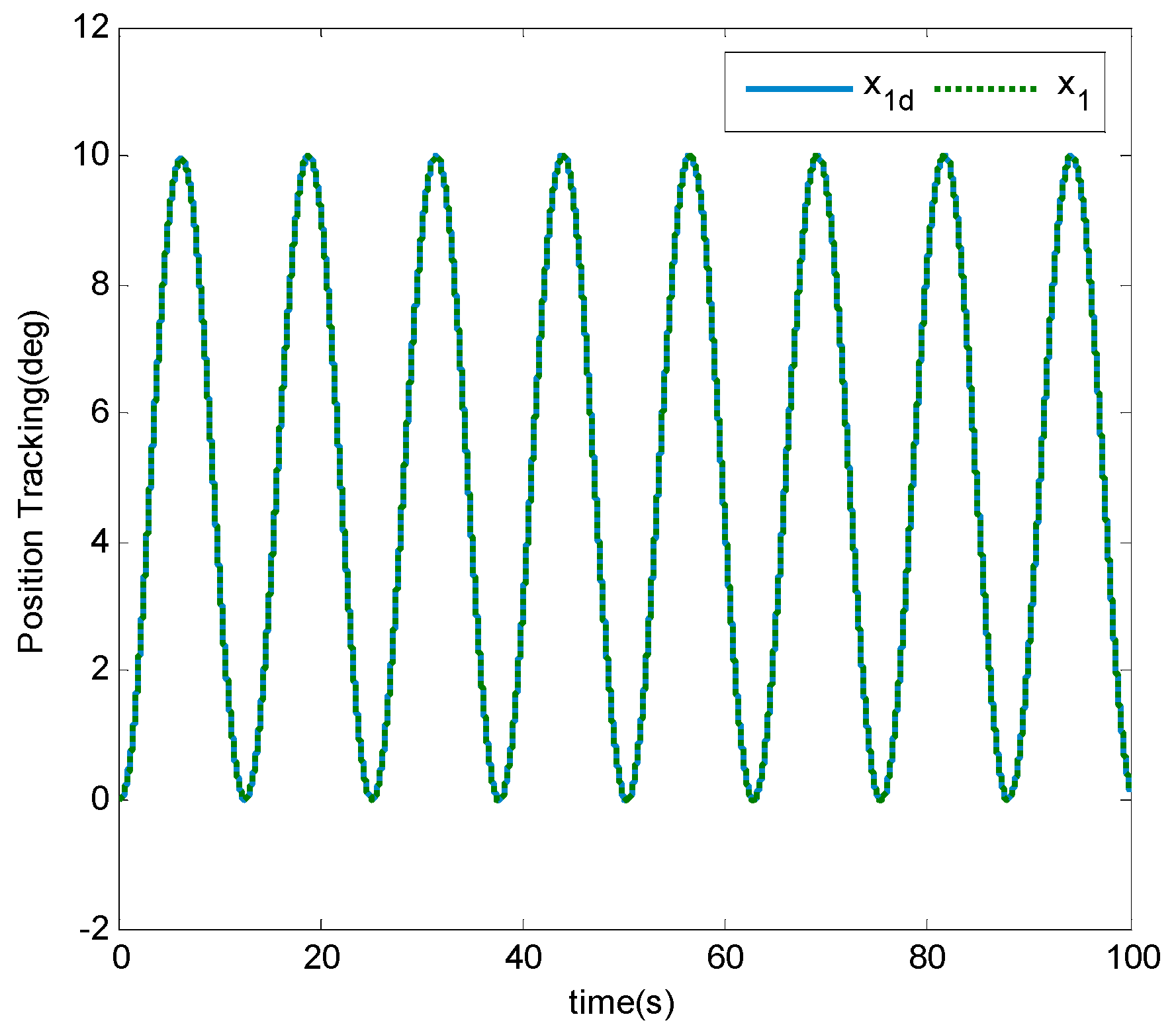
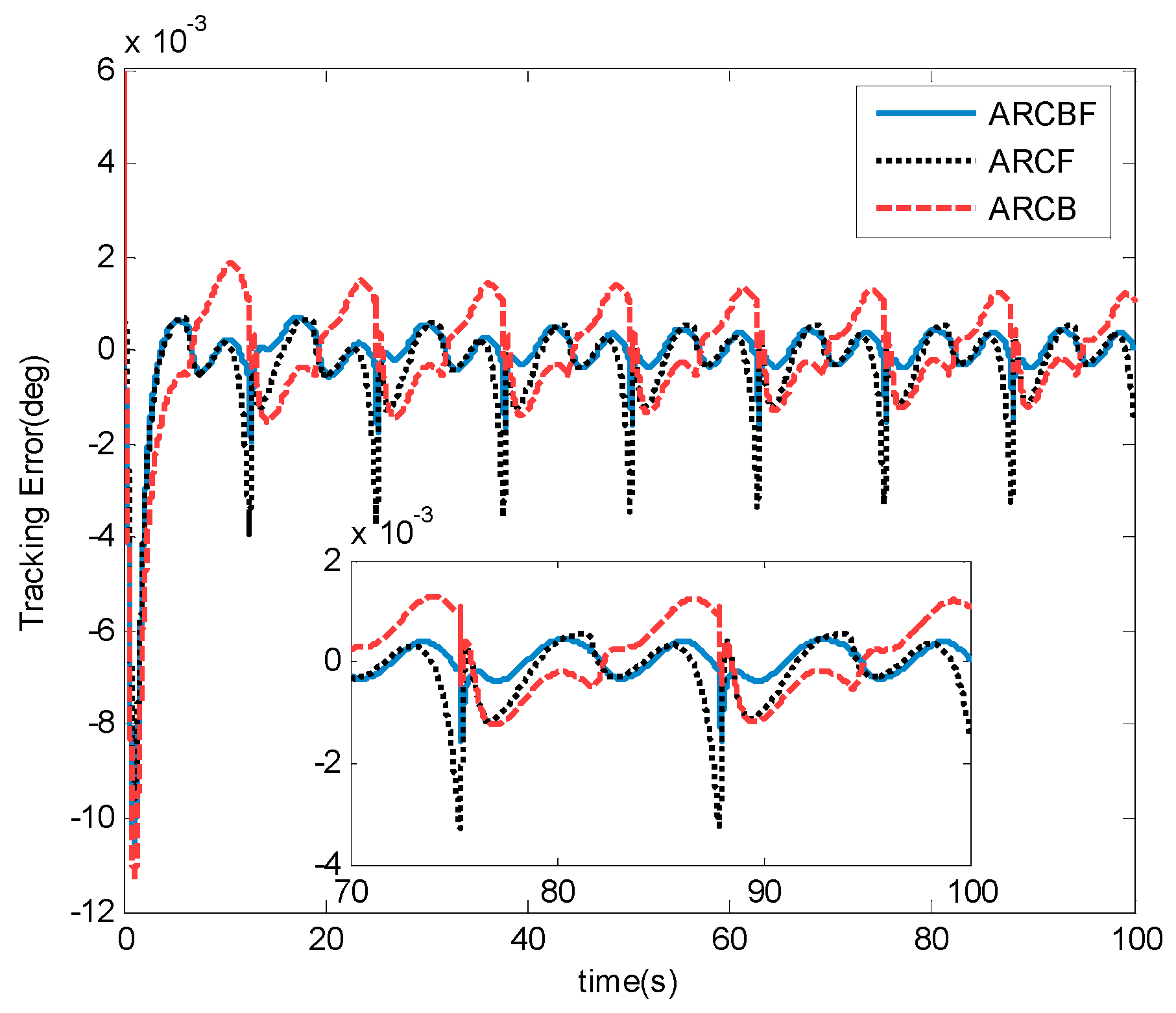
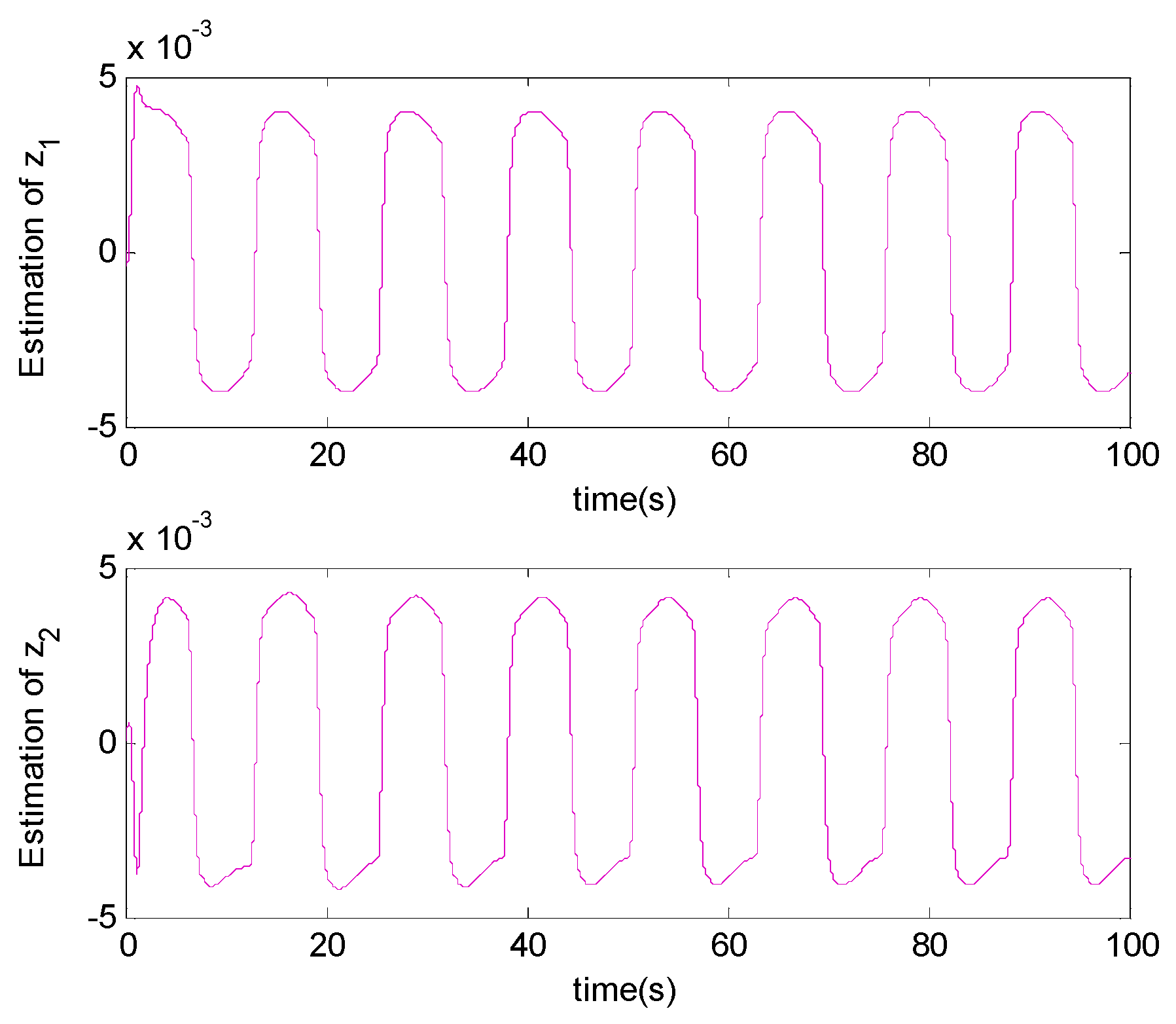
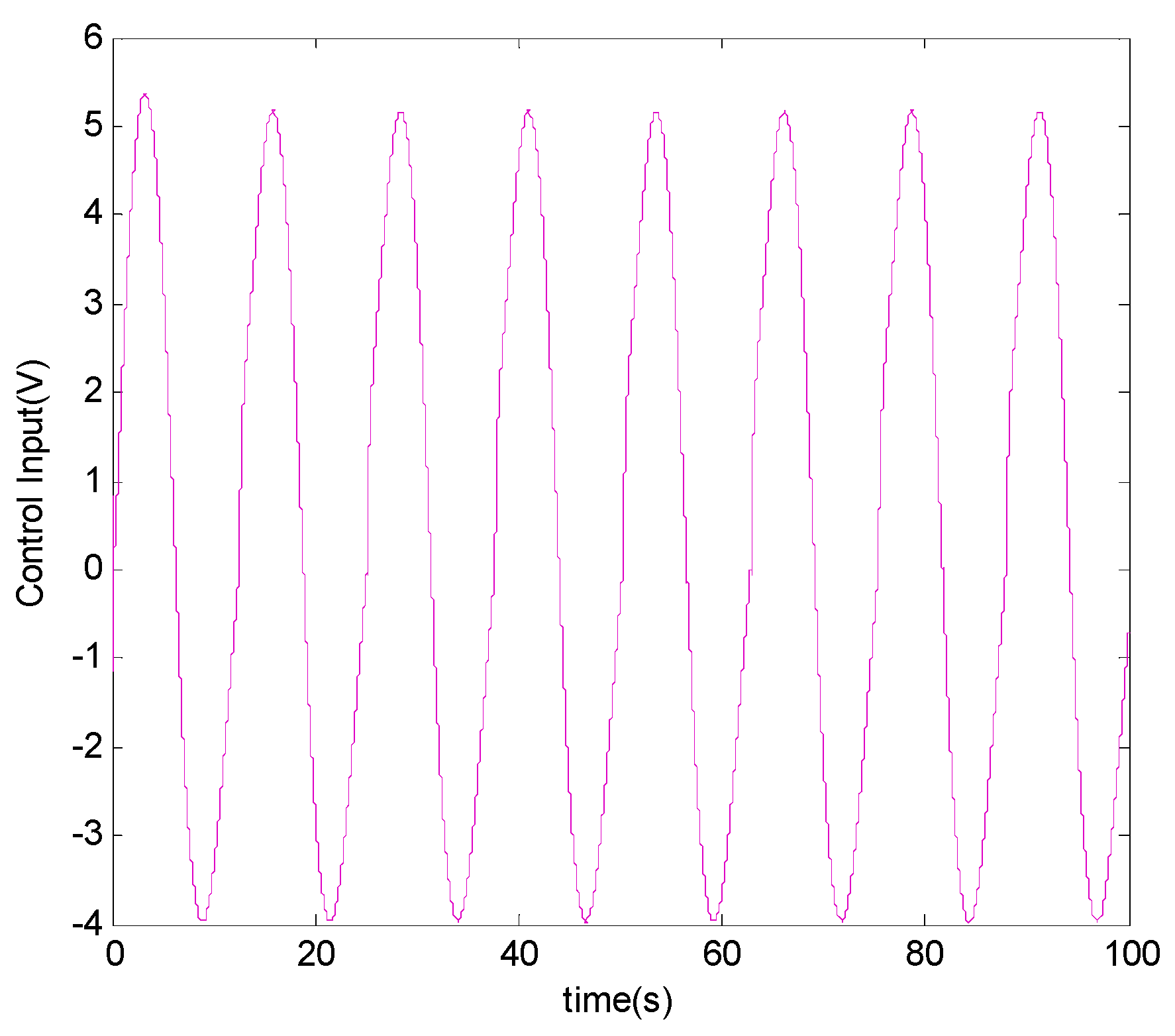
4. Simulation Results and Discussion

To further demonstrate the effectiveness of the proposed control strategy, various simulations are carried out based on the MATLAB/Simulink software. The simulation model parameters of hydraulic manipulation system are chosen as: Ps = 21 MPa, Pr = 0 MPa, A1 = 3.14 × 10⁻² m2, A2 = 1.6 × 10⁻² m2, V01 = 3.1416 × 10⁻⁴ m3, V02 = 3.04 × 10⁻² m3, J = 1.5 × 10⁵ kg·m2, m = 10 t, L1 = 1.6 m, L2 = 2 m, L3 = 3.5 m, L4 = 3 m. The nonlinear function N(x2) is selected as N(x2) = x2/{2 × 10−3 × [tanh(15 × 2) − tanh(1.5 × 2)] + 3 × 10⁻³ × tanh(900 × 2)}. The simulation step size is set to 0.5 ms and the applied disturbance torque d1(t) = 5000sin(t) N·m. The following three controllers are compared:
(1) ARCBF: This is the proposed adaptive robust controller with valve backlash/deadzone compensation and dynamic friction compensation described in Section III;. The following control gains are utilized: k1 = 200, k2 = 5 × 10⁷, k3 = 80. The initial estimate of θ is chosen as θ ^ 0 = [ 5 × 10 5 , 1100 , 2 × 10 5 , 60 , 5 × 10 8 , 0 ] T . The initial estimate of z is z ^ 1 ( 0 ) = z ^ 2 ( 0 ) . The bounds of θ are chosen as θmax = [1 × 10⁷, 1 × 10⁴, 3 × 10⁶, 500, 2 × 10⁹, 0.01]T, θmin = [0, 900, 0, 50, 2 × 10⁸, 0]T. The bounds of z estimation are zmax = 5 × 10⁻³, zmin = −5 × 10⁻³. Parameter adaptation rates are set at Γ = diag{2 × 10⁸, 500, 2 × 10⁵, 2 × 10⁻¹³, 100, 1.5 × 10⁻²⁰}. Friction state learning gains are γ1 = 5 × 10⁻³, γ2 = 5 × 10⁻³.
Remark 3.
The simplification suitable for our simulation is made for the selection of the control gains k1, k2, and k3. We may implement the needed robust control gains in the following two ways. The first method is to pick up a set of values for k1, k2, and k3 rigorously to ensure the theoretical stringency with various prerequisites. However, it increases the complexity of the resulting control law considerably since it may need a significant amount of offline investigating work, sometimes even be impossible. Alternatively, a pragmatic approach is to simply choose k1, k2, and k3 large enough without worrying about the specific prerequisites. In this way, prerequisites will be satisfied for a certain set of values of k1, k2, and k3, at least locally around the desired trajectory to be tracked. In this paper, the second approach is used since it facilitates the online tuning process of gains in implementation.
(2) ARCF: This is the adaptive robust controller same as the proposed ARCBF controller but without considering backlash/deadzone nonlinearities (i.e., let backlash/deadzone ε = 0 in the controller design). Thereby, it can be utilized to verify the significance of the new comprehensive pressure-flow equation compensated in ARCBF. To ensure fair comparison this controller selects the same control gains as ARCBF.
(3) ARCB: The adaptive robust controller without dynamic friction compensation (i.e., let z ^ 1 = z ^ 2 = 0 with γ1 = γ2 = 0). Hence, it will be used to illustrate the effectiveness of the smooth dynamic LuGre friction model proposed in ARCBF. The control parameters are also selected to be consistent with those of ARCBF.
Case 1: The desired position trajectory x1d = 5[1 − cos(0.5t)][1 − exp(−0.1t)]° is first implemented, shown in Figure 3. In this case, the three controllers are tested for two kinds of proportional valves with different backlash values (1 × 10⁻⁶ m and 1 × 10⁻⁵ m). It can be used to illustrate the influence of backlash/deadzone on control performance and the effectiveness of the new comprehensive pressure-flow equation proposed in ARCBF. The compared tracking errors of the three controllers controlled by the two valves are shown in Figure 4 and Figure 5, respectively. As illustrated, the designed control strategy ARCBF has the best tracking performance among the compared controllers since the backlash nonlinearity and nonlinear friction have been compensated effectively. It is interesting to note that, without using the backlash compensation, the control accuracy of ARCF gets worse sharply as the valve backlash increases. Additionally, by comparing the tracking errors between ARCBF and ARCB, it can be inferred that the proposed dynamic friction compensation scheme of ARCBF can effectively suppress the nonlinear friction effects in electrohydraulic systems. Furthermore, the simulation results when ε = 1 × 10⁻⁶ are depicted in Figure 3, Figure 6, Figure 7 and Figure 8. The position tracking performance of ARCBF is shown in Figure 3. From Figure 6, the convergence of the parameter estimation of ARCBF is rather good, which can demonstrate the validity of parameter adaptive law. The estimation of unknown friction states of ARCBF are presented in Figure 7 and the control input is in Figure 8.
Case 2: To further verify the control capability of the proposed control scheme, a higher frequency motion trajectory x1d = [1 − cos(3.14t)][1 − exp(−0.1t)]° is tested and the valve backlash ε = 1 × 10⁻⁵. The position tracking performance of ARCBF is seen from Figure 9 and the compared tracking errors of the three controllers are shown in Figure 10. In this test stage, since the proportional valve switches more frequently, backlash has a greater impact on the tracking performance. However, even in such a high-frequency tracking test, the proposed control strategy is able to compensate for the unexpected effects and achieves the best performance among the three compared controllers, as shown in Figure 10. The parameter adaptation and the friction state estimation, as well as the control input of the proposed ARCBF, are omitted due to space limitation.

5. Conclusions

In this paper, the nonlinear modeling and control of a hydraulic manipulator driven by the proportional valve is studied. Not only system nonlinearities and modeling uncertainties, but also explicit valve backlash/deadzone input nonlinearities in proportional valves, are taken into consideration. To this end, a new comprehensive pressure-flow model is proposed which uniformly indicates both the backlash and deadzone input nonlinearities. Based on this, the pressure dynamics of the hydraulic actuator are established. Additionally, in terms of the manipulator dynamics, with consideration of mechanism nonlinearity and utilizing the smooth LuGre friction model to describe the friction dynamics, a more accurate nonlinear model of the electrohydraulic proportional servo manipulator is then set up. To effectively compensate the nonlinearities and various uncertainties, a high-precision adaptive robust control scheme according to [13,19] is proposed based on the backstepping technology, where a projection-type adaptive law in combination with a robust feedback term is conducted to attenuate parametric uncertainties and uncertain nonlinearities. Based on the Lyapunov stability analysis, the stability of the closed-loop system and the excellent control performance of the proposed controller are proved. Comparative simulation tests are finally obtained to illustrate the effectiveness and priority of the proposed control scheme. As future works, it is worth further testifying the advantages of this new comprehensive pressure-flow model in a practical experimental platform.

Author Contributions

Formal analysis, L.L. and J.Y.; Investigation, Y.J., C.Y. and J.Y.; Methodology, L.L. and J.Y.; Project administration, Z.L.; Writing—original draft, L.L. and Z.L. All authors have read and agreed to the published version of the manuscript.

Funding

This research received no external funding.

Informed Consent Statement

Not applicable.

Data Availability Statement

Data sharing not applicable.

Conflicts of Interest

The authors declare no conflict of interest.

Appendix A

Proof of Theorem 1.
Define a Lyapunov function as
V 1 ( t ) = 1 2 e 1 2 + 1 2 f 1 e 2 2 + 1 2 e 3 2 + 1 2 θ ˜ T Γ 1 θ ˜ + 1 2 γ 1 1 θ 1 z ˜ 1 2 + 1 2 γ 2 1 θ 2 z ˜ 2 2
and its time derivative is
V ˙ 1 = e 1 e ˙ 1 + f 1 e 2 e ˙ 2 + e 3 e ˙ 3 + θ ˜ T Γ 1 θ ^ ˙ + γ 1 1 θ 1 z ˜ 1 z ˜ ˙ 1 + + γ 2 1 θ 2 z ˜ 2 z ˜ ˙ 2
Based on Equations (31), (34) and (40), and noting the condition D1(t) = D2(t) = 0, then we can infer
V ˙ 1 = k 1 e 1 2 + e 1 e 2 k 2 e 2 2 + e 2 e 3 θ 4 θ 4 min k 3 e 3 2 θ ˜ T φ 2 e 2 + θ 1 z ˜ 1 f 3 e 2 θ 2 z ˜ 2 f 4 e 2 + α S 2 e 2 θ ˜ T φ 3 e 3 + θ 4 θ 4 min u S 2 e 3 + θ ˜ T Γ 1 θ ^ ˙ + θ 1 γ 1 1 z ˜ 1 z ˜ ˙ 1 + θ 2 γ 2 1 z ˜ 2 z ˜ ˙ 2
Combing the definition of τ, the property in Equation (26), and noting θ 4 θ 4 min > 1 , we can upper bound V ˙ 1 by
V ˙ 1 k 1 e 1 2 + e 1 e 2 k 2 e 2 2 + e 2 e 3 k 3 e 3 2 + θ 1 z ˜ 1 f 3 e 2 θ 2 z ˜ 2 f 4 e 2 + θ 1 γ 1 1 z ˜ 1 z ˜ ˙ 1 + θ 2 γ 2 1 z ˜ 2 z ˜ ˙ 2
Noting the positive definite matrix defined in Equation (44) and the dynamics given in Equation (30), we obtain
V ˙ 1 e T Λ e + θ 1 γ 1 1 z ˜ 1 { z ^ ˙ 1 [ x 2 N ( x 2 ) z ^ 1 γ 1 f 3 e 2 ] } + θ 2 γ 2 1 z ˜ 2 { z ^ ˙ 2 [ x 2 N ( x 2 ) z ^ 2 + γ 2 f 4 e 2 ] } θ 1 γ 1 1 N ( x 2 ) z ˜ 1 2 θ 2 γ 2 1 N ( x 2 ) z ˜ 2 2
where e = [e1, e2, e3]T. Combing the definition of the learning functions η1 and η2, and the property in Equation (29), we can upper bound the above equation as
V ˙ 1 e T Λ e θ 1 γ 1 1 N ( x 2 ) z ˜ 1 2 θ 2 γ 2 1 N ( x 2 ) z ˜ 2 2
Noting that the nonlinear function N(x2) is always positive, then
V ˙ 1 e T Λ e λ min ( Λ ) ( e 1 2 + e 2 2 + e 3 2 ) W
where λmin(Λ) is the minimal eigenvalue of matrix Λ. Therefore, V1L and WL2. Based on the definition of V1 in Equation (A1), it can be inferred that e 1 , e 2 , e 3 , θ ˜ , z ˜ 1 , z ˜ 2 are bounded; from assumptions 1 and 2, we can infer that x is bounded; based on Equation (34) and assumption 2, the boundness of e ˙ 2 is; thus, obtained; from Equation (33), we can easily obtain that α ˙ 2 is bounded. Then the boundedness of the control input u can be concluded. Hence, all system signals are bounded under closed-loop operation.
From the above analysis, combining the dynamics of e1, e2, e3, it is easy to check that the time derivative of W is bounded, thus W is uniformly continuous. By applying Barbalat’s lemma [28], W→0 as t→∞, which leads to the results in Theorem 1. □

Appendix B

Proof of Theorem 2.
If there exists unmodeled disturbances in the system, the time derivative of V2 defined in Equation (46) can be presented by
V ˙ 2 k 1 e 1 2 + e 1 e 2 k 2 e 2 2 + e 2 e 3 k 3 e 3 2 + e 2 [ θ ˜ T φ 2 + θ 1 z ˜ 1 f 3 θ 2 z ˜ 2 f 4 + D 1 ( t ) + α S 2 ] + e 3 [ θ ˜ T φ 3 + θ 4 θ 4 min u S 2 + D 2 ( t ) ]
Combining the conditions in Equations (37) and (43), we can infer that
V ˙ 2 k 1 e 1 2 + e 1 e 2 k 2 e 2 2 + e 2 e 3 k 3 e 3 2 + ε
Based on the definition of Λ in Equation (44), the inequality becomes
V ˙ 2 λ min ( Λ ) ( e 1 2 + e 2 2 + e 3 2 ) + ε κ V + ε
By integrating the aforementioned equation, the inequality in Equation (47) can be proved. Then, V2 is bounded (i.e., e1, e2, e3 are bounded). Similar to the proof in Theorem 1, the boundness of u can also be obtained. □

References

  1. Lu, L.; Yao, B. Energy-Saving Adaptive Robust Control of a Hydraulic Manipulator Using Five Cartridge Valves with an Accumulator. IEEE Trans. Ind. Electron. 2014, 61, 7046–7054. [Google Scholar] [CrossRef]
  2. Seron, J.; Martinez, J.L.; Mandow, A.; Reina, A.J.; Morales, J.; Garcia-Cerezo, A.J. Automation of the Arm-Aided Climbing Maneuver for Tracked Mobile Manipulators. IEEE Trans. Ind. Electron. 2013, 61, 3638–3647. [Google Scholar] [CrossRef]
  3. Lane, D.M.; Dunnigan, M.W.; Clegg, A.C.; Dauchez, P.; Cellier, L. A comparison between robust and adaptive hybrid position/force control schemes for hydraulic underwater manipulators. Trans. Inst. Meas. Control 1997, 19, 107–116. [Google Scholar] [CrossRef]
  4. Koivumaki, J.; Mattila, J. Stability-Guaranteed Force-Sensorless Contact Force/Motion Control of Heavy-Duty Hydraulic Manipulators. IEEE Trans. Robot. 2015, 31, 918–935. [Google Scholar] [CrossRef]
  5. Yao, J.; Yang, G.; Jiao, Z. High dynamic feedback linearization control of hydraulic actuators with backstepping. Proc. Inst. Mech. Eng. Part. I J. Syst. Control Eng. 2015, 229, 728–737. [Google Scholar] [CrossRef]
  6. Kim, W.; Won, D.; Tomizuka, M. Flatness-Based Nonlinear Control for Position Tracking of Electrohydraulic Systems. IEEE/ASME Trans. Mechatron. 2014, 20, 197–206. [Google Scholar] [CrossRef]
  7. Choi, Y.-S.; Choi, H.H.; Jung, J.-W. Feedback Linearization Direct Torque Control With Reduced Torque and Flux Ripples for IPMSM Drives. IEEE Trans. Power Electron. 2016, 31, 3728–3737. [Google Scholar] [CrossRef]
  8. Al Aela, A.M.; Kenne, J.-P.; Mintsa, H.A. A Novel Adaptive and Nonlinear Electrohydraulic Active Suspension Control System with Zero Dynamic Tire Liftoff. Machines 2020, 8, 38. [Google Scholar] [CrossRef]
  9. Lin, Y.-T.; Tseng, C.-Y.; Kuang, J.-H.; Hwang, Y.-M. A Design Method for a Variable Combined Brake System for Motorcycles Applying the Adaptive Control Method. Machines 2021, 9, 31. [Google Scholar] [CrossRef]
  10. Noghredani, N.; Pariz, N. Robust adaptive control for a class of nonlinear switched systems using state-dependent switching. SN Appl. Sci. 2021, 3, 290. [Google Scholar] [CrossRef]
  11. Homayounzade, M. Adaptive robust output-feedback boundary control of an unstable parabolic PDE subjected to unknown input disturbance. Int. J. Syst. Sci. 2021, 1–14. [Google Scholar] [CrossRef]
  12. Kissai, M.; Monsuez, B.; Mouton, X.; Martinez, D.; Tapus, A. Adaptive Robust Vehicle Motion Control for Future Over-Actuated Vehicles. Machines 2019, 7, 26. [Google Scholar] [CrossRef] [Green Version]
  13. Zhao, D.; Wang, Y.; Xu, L.; Wu, H. Adaptive Robust Control for a Class of Uncertain Neutral Systems with Time Delays and Nonlinear Uncertainties. Int. J. Control Autom. Syst. 2021, 1–13. [Google Scholar] [CrossRef]
  14. Hu, C.; Yao, B.; Wang, Q. Performance-Oriented Adaptive Robust Control of a Class of Nonlinear Systems Preceded by Unknown Dead Zone with Comparative Experimental Results. IEEE/ASME Trans. Mechatron. 2011, 18, 178–189. [Google Scholar] [CrossRef]
  15. Jia, X.; Xu, S.; Qi, Z.; Zhang, Z.; Chu, Y. Adaptive output feedback tracking of nonlinear systems with uncertain nonsymmetric dead-zone input. ISA Trans. 2019, 95, 35–44. [Google Scholar] [CrossRef] [PubMed]
  16. Jia, X.; Xu, S.; Zhang, Z.; Cui, G. Output feedback robust stabilization for uncertain nonlinear systems with dead-zone input. IET Control Theory Appl. 2020, 14, 1828–1836. [Google Scholar] [CrossRef]
  17. Zhang, Z.; Xu, S.; Zhang, B. Asymptotic Tracking Control of Uncertain Nonlinear Systems with Unknown Actuator Nonlinearity. IEEE Trans. Autom. Control. 2014, 59, 1336–1341. [Google Scholar] [CrossRef]
  18. Ma, Z.; Ma, H. Decentralized adaptive NN output-feedback fault compensation control of nonlinear switched large-scale systems with actuator dead-zones. IEEE Trans. Syst. Man Cybern. Syst. 2018, 1–13. [Google Scholar] [CrossRef]
  19. Mohanty, A.; Yao, B. Integrated Direct/Indirect Adaptive Robust Control of Hydraulic Manipulators with Valve Deadband. IEEE/ASME Trans. Mechatron. 2010, 16, 707–715. [Google Scholar] [CrossRef]
  20. Zhou, J.; Wen, C.; Zhang, Y. Adaptive Output Control of Nonlinear Systems with Uncertain Dead-Zone Nonlinearity. IEEE Trans. Autom. Control 2006, 51, 504–511. [Google Scholar] [CrossRef]
  21. Deng, W.; Yao, J.; Ma, D. Robust adaptive precision motion control of hydraulic actuators with valve dead-zone compensation. ISA Trans. 2017, 70, 269–278. [Google Scholar] [CrossRef] [PubMed]
  22. Lewis, F.; Tim, W.K.; Wang, L.-Z.; Li, Z. Deadzone compensation in motion control systems using adaptive fuzzy logic control. IEEE Trans. Control Syst. Technol. 1999, 7, 731–742. [Google Scholar] [CrossRef]
  23. Yao, J.; Deng, W.; Jiao, Z. Adaptive Control of Hydraulic Actuators with LuGre Model-Based Friction Compensation. IEEE Trans. Ind. Electron. 2015, 62, 6469–6477. [Google Scholar] [CrossRef]
  24. Yao, B.; Tomizuka, M. Adaptive robust control of SISO nonlinear systems in a semi-strict feedback form. Automatica 1997, 33, 893–900. [Google Scholar] [CrossRef]
  25. Makkar, C.; Dixon, W.; Sawyer, W.; Hu, G. A new continuously differentiable friction model for control systems design. In Proceedings of the 2005 IEEE/ASME International Conference on Advanced Intelligent Mechatronics, Monterey, CA, USA, 24–28 July 2005; IEEE: New York, NY, USA, 2006; pp. 600–605. [Google Scholar]
  26. Eryilmaz, B.; Wilson, B.H. Unified modeling and analysis of a proportional valve. J. Frankl. Inst. 2006, 343, 48–68. [Google Scholar] [CrossRef]
  27. Manring, N.D. Hydraulic Control Systems; John Wiley & Sons: Hoboken, NJ, USA, 2005; pp. 224–228. [Google Scholar]
  28. Krstic, M.; Kanellakopoulos, I.; Kokotovic, P. Nonlinear and Adaptive Control Design; Wiley: New York, NY, USA, 1995. [Google Scholar]
Figure 1. The motion schematic diagram of hydraulic lifting manipulator.
Machines 09 00057 g001
Figure 2. The schematic diagram of the flow of the proportional valve.
Machines 09 00057 g002
Figure 3. The position tracking of ARCBF as ε = 1 × 10⁻⁶.
Machines 09 00057 g003
Figure 4. The compared tracking errors of the three controllers as ε = 1 × 10⁻⁶.
Machines 09 00057 g004
Figure 5. The compared tracking errors of the three controllers as ε = 1 × 10⁻⁵.
Machines 09 00057 g005
Figure 6. The parameter adaptation of ARCBF as ε = 1 × 10⁻⁶.
Machines 09 00057 g006
Figure 7. The friction state adaptation of ARCBF as ε = 1 × 10⁻⁶.
Machines 09 00057 g007
Figure 8. The control input of ARCBF as ε = 1 × 10⁻⁶.
Machines 09 00057 g008
Figure 9. The position tracking of ARCBF in case 2.
Machines 09 00057 g009
Figure 10. The compared tracking errors of the three controllers in case 2.
Machines 09 00057 g010
Publisher’s Note: MDPI stays neutral with regard to jurisdictional claims in published maps and institutional affiliations.

