Article

Motion Planning of Ground Simulator for Space Instable Target Based on Energy Saving

1
School of Mechanical Science and Engineering, Huazhong University of Science and Technology, Wuhan 430074, China
2
Shenyang Institute of Automation, Chinese Academy of Sciences, Shenyang 110016, China
3
Institutes for Robotics and Intelligent Manufacturing, Chinese Academy of Sciences, Shenyang 110169, China
4
Aerospace System Engineering Shanghai, Shanghai 201109, China
5
Shanghai Aerospace Chemical Engineering Institute, Huzhou 313000, China
*
Author to whom correspondence should be addressed.
Machines 2021, 9(12), 368; https://doi.org/10.3390/machines9120368
Submission received: 12 November 2021 / Revised: 8 December 2021 / Accepted: 15 December 2021 / Published: 18 December 2021
(This article belongs to the Topic Motion Planning and Control for Robotics)

Abstract

:
In order to achieve the high-precision motion trajectory in ground experiment of space instable target (SIT) while reducing the energy consumption of the motion simulator, a robot motion planning method based on energy saving is proposed. Observable-based ground robot motion experiment system for SIT is designed and motion planning process is illustrated. Discrete optimization mathematical model of energy consumption of motion simulator is established. The general motion form of the robot joints in ground test is given. The optimal joint path of motion simulator based on energy consumption under discontinuous singularity configuration is solved by constructing the complete energy consumption directed path and Dijkstra algorithm. An improved method by adding the global optimization algorithm is used to decouple the coupled robot joints to obtain the minimum energy consumption path under the continuous singularity configuration of the motion simulator. Simulations are carried out to verify the proposed solution. The simulation data show that total energy saving of motion simulator joints adopting the proposed method under the condition of non-singularity configuration, joints coupled motion with continuous singularity configuration, and coexistence of non-singularity path and continuous singularity path are, respectively, 72.67%, 28.24%, and 62.23%, which proves that the proposed method can meet the requirements of ground motion simulation for SIT and effectively save energy.

1. Introduction

As unstable targets in space continue to increase and become more threatening, maneuvering tasks, such as on-orbit removal, have become more and more urgent [1,2,3,4]. Space instable targets are objects to be manipulated in orbit, such as satellites and space debris, in space operation missions. The movement of SIT is complicated, and their manipulation task is also difficult [5]. In order to verify the feasibility of the space control method and optimize the control algorithm, it is necessary to conduct ground manipulation simulation experiments of SIT [6,7]. The primary task of the ground simulation test is to accurately simulate the relative spatial movement and relative attitude motion between SIT and space operation aircraft.
A serial robot with multi-DOF, widely used in areas such as grinding, polishing, and parts processing, has the advantages of a large range of pose motion and high repeat positioning accuracy. It is an effective method to achieve the given motion of SIT in ground test platform through using six-DOF industrial robot [8,9]. During simulating given space movement in the ground test, it is necessary to optimize the robot path on the premise that the simulation accuracy meets the requirements, and at the same time ensure the dynamic characteristics of the simulator. With the increasingly tense global energy situation, the optimization and control of robot energy consumption has gradually become an important goal in industrial systems [10].
Many motion planning methods and trajectory optimization algorithms have been proposed and studied to achieve smooth movement, obstacle avoidance, and flexible contact collisions in different application scenarios [11,12,13,14,15]. Interpolation, curve fitting the trajectory of the robot joint angular displacement or the cartesian pose of the robot end target position, generally including polynomial curve, Bézier spline, and NURBS curve, is adopted to smooth the path in robot motion planning to reduce acceleration shock and movement jitter [16,17]. In high-precision machining of parts, Pavel [18] adopts the analytic geometry method on the basis of the symmetries in the Euclidean plane and achieves a trajectory error of less than 5% in experiments, which proves the feasibility of generating complex processing motion for robot. Modelled predictive control approach, based on vision system and linear interpolation, is applied for the task of ball-catching to generate robot real-time trajectory [19]. Aiming at the multi-path optimization issue, R.A. [20] uses genetic algorithms to search for the shortest path without collision, which connects preset points in the robot’s task space. Chaos enhanced accelerated particle swarm optimization (CAPSO) is developed by Taghavifar [21] to plan the optimal path of a wheeled robot, and ensures the shortest path from the starting point to the target position by avoiding collision with static and dynamic obstacles. The improved algorithm combining Dijkstra algorithm or A* algorithm with other algorithms can effectively perform the shortest path search, which has the advantages of a small calculation and fast convergence speed, and is used in varieties of scenarios of robot operations [22,23,24,25,26].
In terms of optimal motion planning combined with minimal energy consumption and robot operation tasks, many implementation methods have emerged. One DoF mechatronic system is studied by Giovanni to reduce the energy consumption and the minimum energy consumption conditions have been found in a closed form taking into account the chance of recovering the braking energy [27]. A robot configuration selection method based on the lowest power consumption is studied by Abdullah and verified through a straight-line scenario and a square-path scenario, which achieve the goal of optimizing the calculated joint configuration [28]. Luo uses Chebyshev interpolation points and direct iteration method to plan the trajectory of industry robotic manipulators for energy minimization, and the method is applied to the three-link plane mechanism, which obtained optimal joint angles under the premise that the start and end points of the movement are known [29]. A task-related analysis is used by Scalera to enhance the energy efficiency of a 4-DOF parallel robot [14]. Carabin adopts the trajectory planning mean, which is on the basis of electromagnetic field model and the derivation of the energy formulation, to realize the minimum-energy consumption of the Cartesian robot [30]. Bitar proposed a method of obtaining energy-optimized trajectory planning while managing obstacle constraints for ASVs [31]. The enhanced bacterial foraging optimization algorithm is researched by Abbas and applied to path planning in two-dimensional motion space [32]. An artificial bee colony algorithm and a genetic algorithm is studied to optimize the working path length and welding time of the welding robot, which minimizes the total amount of robot joint movement [33,34]. Sathiya [35] takes the execution time and execution tasks of mobile robots as the optimization goals, and proposes the application of evolutionary algorithms to achieve multi-objective optimization in trajectory planning. Under the conditions of kinematics and dynamics constraints, Amruta [36] presents the EMOTLBO approach to get the best joint motion that defines the weld path, which effectively enhances the efficiency of the robot in operation tasks. Wang [37] applies the improved whale optimization algorithm to obtain the constant velocity motion of the robot end effector, which improves the processing efficiency and quality of the grinding task. Under the working conditions of the power generation mode and the energy exchange, Christian [38] proposes an energy-based robot model based on B-spline functions and realizes the optimization of energy between different joints. Aiming at the robot PTP motion planning without collision, Francisco [39] uses a third-order polynomial method to fit the joint space motion, which obtains an approximate optimal time trajectory and considers the constraint of energy consumed.
Inspired by the above-mentioned research works and considering the particularity of ground simulation of space instability targets, there are still several issues that need to be studied and solved. Firstly, it is hard to completely avoid robot singularity configuration due to the large coverage of the motion range in ground simulation experiment of SIT [40,41], which makes the motion optimization with singular position particularly important. Secondly, although the intelligent optimization algorithm based on the global search is sufficiently robust to acquire the optimized path, the optimization result is more likely to converge prematurely in the process of processing multi-objective optimization [42], which will cause the problem of difficulty in motion reproduction and simulation validity when the robot exists with different error sources. Furthermore, there may be multiple optimal motion paths or cases where the sub-optimal path is better than the optimal path on certain evaluation functions and the path search algorithm needs to be improved accordingly. Finally, the spin motion of SIT on orbit is not restricted, that is, it can be rotated infinitely, in contrast to the limited simulation of rotational motion subjected to robot structure. How to achieve the simulation of spin motion as much as possible with minimal energy consumption through the combined motion and motion optimization of the robot joints is also an issue of motion planning of the SIT movement simulation robot, especially when singularity causes multi-axis coupling.
Focusing on the characteristics of ground motion simulation of SIT and the mentioned challenges above, the study proposes an optimization method of simulator motion path including a singularity configuration based on energy saving. Ground motion planning of SIT is performed through motion mapping and path optimization of motion simulation robots. The local optimal solution is avoided through path search algorithm on the basis of constructing a complete directional motion path of energy consumption. The versatility of ground motion simulation of SIT is achieved using the presented approach and it enhances the authenticity of the ground experiment and reduces the energy consumption of the ground system.
The rest of the paper is organized as follows: ground motion planning method of SIT and motion optimization model of SITMSR are described in Section 2 and Section 3, respectively; solution to the optimal joint trajectory of SITMSR and results obtained by a series of simulations are presented in Section 4 and Section 5, respectively; and conclusions are drawn in Section 6.

2. Ground Motion Planning Method of SIT

2.1. Ground Motion Simulation State Description of SIT

The motion of SIT in space is in the free-floating state, which can be decomposed into attitude movement and centroid translation movement. The attitude general form of SIT is spin movement around the axis of maximum inertia and the nutation angle will change with the pose controllability in the close-range orbit and attitude tracking stage and the final approach stage according to space dynamics [4]. Position movement is the three-dimensional space motion obtained after task-level trajectory planning. Therefore, the movement of the SIT is a motion of 6-DOF in space. The motion simulation state of SIT in the ground experiment is described in Figure 1.
Where O GS X GS Y GS Z GS is the inertial coordinate system of the ground experiment system, O IT X IT Y IT Z IT is the framework fixed in SIT, r GS denotes centroid vector of SIT in O GS X GS Y GS Z GS . φ IT , θ IT and ψ IT are precession angle, nutation angle, and spin angle defined in O IT X IT Y IT Z IT .
To ensure the effectiveness of the ground test, the angular velocity and translation velocity are required to meet the given precision. The expressions of ground simulation motion accuracy of SIT are as follows:
| V ITa GS r ˙ IT GS | γ v
| ω ITa IT ω IT IT | γ ω
where V ITa GS and r ˙ IT GS are the actual velocity and the given velocity of the mass center of SIT defined in O GS X GS Y GS Z GS during the ground simulation experiment, respectively. ω ITa IT and ω IT IT are the actual angular velocity and the given angular velocity. γ v and γ ω are the given velocity error and angular velocity error.
The observable angular velocity in the ground test can be obtained by projecting Equation (2) in O GS X GS Y GS Z GS . Taking ω ITa IT as an example, we get:
ω ITa GS IT = T GS IT T φ θ R ˙ Eu
where ω ITa GS IT is the projection of ω ITa IT in O GS X GS Y GS Z GS , T GS IT is the homogeneous transformation matrix from O IT X IT Y IT Z IT to O GS X GS Y GS Z GS , T φ θ is the angular velocity projection matrix, and R ˙ Eu = [ φ ˙ IT θ ˙ IT ψ ˙ IT ] T .
Through the analysis of the simulation state of the ground motion of SIT, it can be seen that the state exists where projection of the centroid velocity and angular velocity of the ground motion in O GS X GS Y GS Z GS is not zero, which means 6-DOF motion of SIT should be simulated in the ground test. In other words, velocity motion and angular velocity motion of SIT in the ground test possess the generality of space motion.

2.2. Composition and Motion Planning Process of SITMSRS

Compared with parallel robot and cooperative manipulator, 6-DOF industrial robots have the characteristics of large motion range, high load capacity, and high motion accuracy. At the same time, they have the advantages of small envelope space, high technology maturity, and low cost over a truss robot. Therefore, the 6-DOF industrial robot system is chosen to simulate the motion of SIT in the ground experiment. The space instable target motion simulation robot system (SITMSRS), mainly composed of a 6-DOF industrial robot (SITMSR), the space instable target simulator (SITS), a motion control computer, and electrical system, is designed to achieve the planned positions and attitudes given above. SITS is installed on the end flange of SITMSR, which equipped with capture ring, on-board analogue elements, and six-axis force/torque sensor. The capture ring is the capture object for the space manipulator to carry out takeover tasks during the ground test. The capture ring and on-board analogue elements are used as recognition features for motion parameter estimation and 3D reconstruction. The six-axis force/torque sensor can measure the forces and moments applied on SITS. SITS need to have the same properties as the real SIT, including the width and height of the SIT, the geometric size and material of the capture ring, etc. The motion control computer is used to realize the planning and optimization of the motion trajectory and interact with the robot system. The composition of designed SITMSRS is shown in Figure 2.
The spatial movement of the centroid of the SIT and attitude movement, including precession, nutation, and spin planned by the motion control computer, can be achieved by joint compound motion of SITMSR to form the general motion form of SIT. It is hard to control angular velocity of SITMSR joints directly. Nevertheless, the spatial position r IT GS and attitude P IT GS can be obtained by integrating the velocity and angular velocity of the SIT in the ground simulation experiment. Thus, the ground motion of the SIT is simulated by controlling the angular displacement motion of the SITMSR joints.
Since there are multiple solutions for the angular displacement of robot joints under the same position and pose of the SIT, it is necessary to optimize the joint movement of SITMSR to save energy consumption. The input to robot motion control is based on discrete point planning, and when the number of discrete points Ndis is constant, the motion planning of the SIT is transformed into the path planning and optimization problem of the SITMSR joint motions. The motion planning flowchart of SITMSRS is indicated in Figure 3.
From Figure 3, the joint path optimization of the SITMSR based on energy saving is the crucial part of the above motion planning process and needs to be further studied in detail.

3. Motion Optimization Model of the SITMSR Based on Energy Saving

3.1. Mathematical Model of Joint Trajectory of the SITMSR

Define qi (i = 1, 2, ⋯, 6 as generalized coordinate of SITMSR and SITMSR kinematics is modeled by the D-H method. Suppose OX 0 Y 0 Z 0 is the base coordinate system and OX i Y i Z i is the joint coordinate system. The definition of DH parameters and joint coordinate systems of SITMSR are shown in Figure 4.
Suppose the centroid coordinates of SIT is r c and it can be calculated as follows:
T 6 0 = T s T s 6 - 1
T 6 0 = f ( q 1 , q 2 , q 3 , q 4 , q 5 , q 6 , a 1 , a 2 , a 3 , d 1 , d 4 , α 1 , α 3 , α 4 , α 5 )
T s = [ P IT GS r IT GS 0 1 ]
T s 6 = [ I 3 × 3 r c 0 1 ]
where T 6 0 is the homogeneous transformation matrix of SITMSR and T s is the position and attitude matrix planned of SIT in the ground experiment. a1, a2, a3, d1, and d4 are the geometric parameters of the coordinate transformation and α1, α3, α4, and α5 are the rotation angles of the joint coordinate system using D-H method as shown in Figure 4.
The value of qi, which is also the joint angular displacement of each axis of the SITMSR, can be obtained by solving Equations (4)–(7).
The motion control of the SITMSR is based on the displacement control of the discrete points in the ground experiment. The angular displacement is discretized based on the dispersing of the given trajectory. The approach of polynomial fitting is used to carry out the continuity of the discrete path of the SITMSRS.

3.2. Discrete Optimization Mathematical Model of Energy Consumption

SITMSR need to accurately simulate the given motion of SIT firstly, which meet the given motion simulation error. Secondly, it is necessary to ensure the total energy consumption of the SITMSR axes is low during the simulating trajectory. Additionally, in order to avoid violent measurement data jitter of the six-axis force/torque sensor measurement values, the smoothness of the movement of the SITS is also required. Based on the above considerations, the objective function in the mathematical model of motion optimization of SITMSR can be described as follows:
min F = [ f 1 f 2 ] = [ N d i s t p N d i s 1 i = 1 N q j = 1 N d i s | T q i , j q ˙ i , j | ]
where t p is the given motion simulation time, q ˙ i , j is the joint angular velocity, Nq is the number of SITMSR joint axes, Ndis is the number of discrete points of a given trajectory of SITS, q ˙ i , j is the angular velocity of qj at the discrete point j, and T q i , j is the joint drive torque when the angular displacement is qi,j.
The constraint conditions corresponding to above objective function are:
s . t . { | V ITa GS r ˙ IT GS | γ v | ω ITa IT ω IT IT | γ ω | M ITa IT M IT IT M IT IT | γ M q i , j [ q i m i n , q i m a x ] t p | q i , j q i , j - 1 | N t r a j 1 q ˙ i m a x t p q ˙ i , j N t r a j 1 q ¨ i m a x
where M ITa IT and M IT IT are the values of the six-axis force/torque sensor in SITS when the trajectory is given and when the trajectory is planned, respectively. γ M is the allowable value of relative error between M ITa IT and M IT IT , N t r a j is the number of discrete points from the joint path to the joint trajectory. q ˙ i m a x and q ¨ i m a x are the maximum allowable values of the joint angular velocity and the angular acceleration, respectively.
SITMSR dynamics equations in discrete form using Newton–Euler algorithm is presented in Equation (10).
T q i , j = T i + 1 i × T q i + 1 , j f i , j × r i 1 , c i + T i + 1 i × f i + 1 , j × r i , c i + ω i , j × ( I i × ω i , j ) + I i × a i , j
where f i , j is the interaction force between link i and link i + 1 at the discrete point j of the trajectory, r i , c i is the position vector of the gravity center of link i in the framework of OXiYiZi, ω i , j is the angular velocity of the link i, I i is the inertial tensor matrix and a i , j is the linear acceleration at the end point of the link i.
SITMSR is considered as rigid bodies in the process of dynamic modeling, and the effects of viscous force are ignored. The measurements for six-axis force/torque can be obtained by solving the dynamics model of SITS based on Newton–Euler algorithm. The expressions of f i , j , r i , c i , ω i , j , and a i , j are obtained in [28]. f 7 , j and τ 7 , j in the framework of OX6Y6Z6 can be written as:
( f 7 , j , τ 7 , j ) = [ ( G SITS , 0 , 0 ) , r c × f 7 , j ]
where GSITS is the gravity of SITS.

4. Solution to the Optimal Joint Trajectory of SITMSR

4.1. The General Form of Joint Motion Trajectories

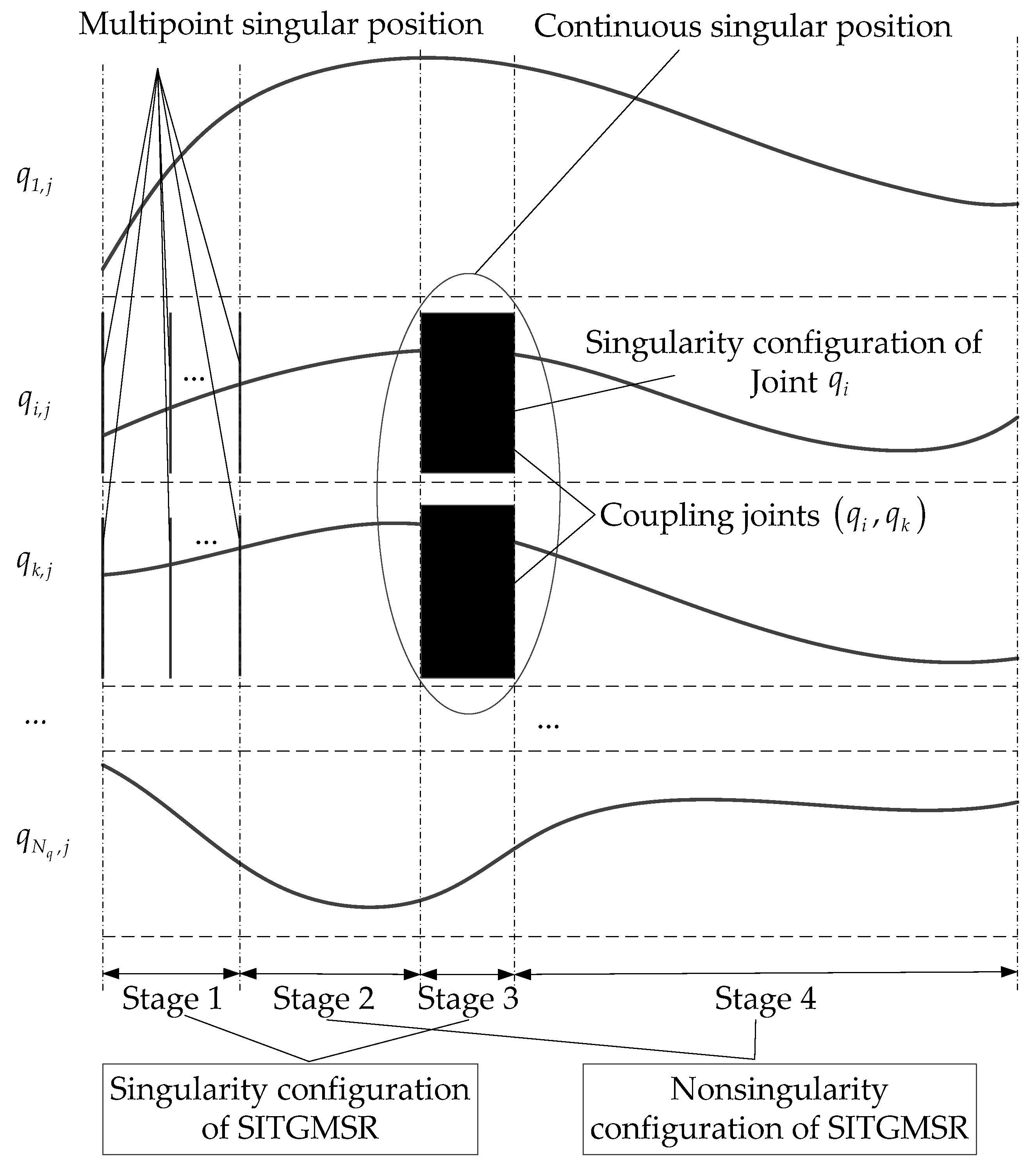
For the planned motion of SITS is complex and diverse, it leads to the generality of the motion of SITMSR. As a result, the compound situations of singularity configuration and non-singularity configuration of SITMSR should be considered. The singularity can be judged by the full rank of Jacobian matrix, which can also be quickly determined by using three singular factors extracted from the joint expressions of the Jacobian matrix. Another method is to judge whether there is a problem of DOF degradation. The general forms of the SITMSR joint motion trajectories are seen in Figure 5.
To facilitate the solution of the optimal trajectory, the joint movement above can be segmented into paths with non-singularity configuration (Stages 2 and 4 in Figure 5) and paths with singularity configuration. Paths with singularity configuration are divided into trajectory with multipoint singular position (Stage 1 in Figure 5) and trajectory with continuous singular position (Stage 3 in Figure 5). Although joint qi and qk have constraints, respectively, even under the premise of coupled angular displacement constraints, there are infinite sets of solutions for their joint angular displacements. If the robot continues to run in this condition, then the robot is in the continuous singularity configuration as shown in Stage 3. We solved each segment of the optimal path separately, and, finally, merged the optimal solutions of the multiple segments to obtain the optimal trajectory of SITMSR under the general path form of SIT in the ground experiment.

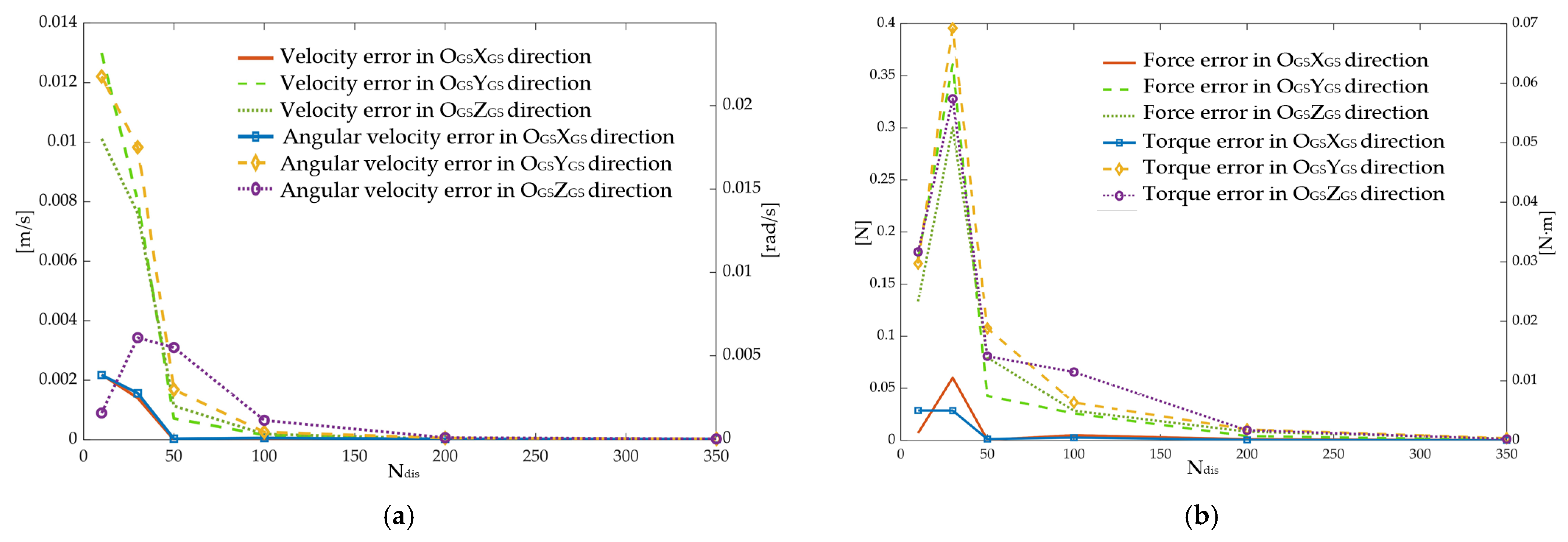
4.2. Optimal Selection of Ndis

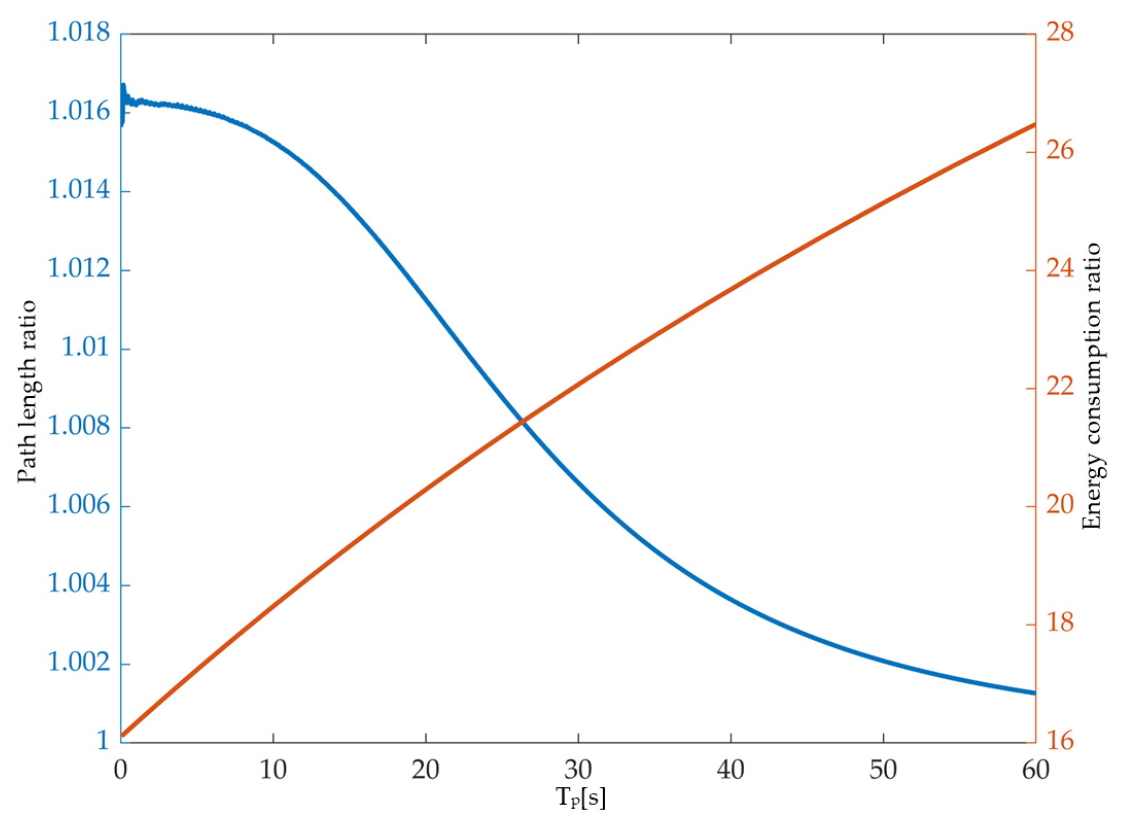
From the motion planning of SITMSRS and motion optimization model based on energy saving, it can be seen that Ndis is closely related to the simulation accuracy of a given motion trajectory. The ground motion simulation error of SIT is large when Ndis is small, which, obviously, does not meet the simulation requirements. This is because when the motion of SITS is determined, the fewer the number of discrete points, the greater the deviation of the motion trajectory between two adjacent discrete points, and the greater the error between the corresponding velocity and angular velocity and the ideal state. The trajectory simulation precision will continue to improve as Ndis continues to increase and it is paradoxical that the total number of paths will also increase exponentially leading to lower efficiency in solving the optimal trajectory.
Motion planning of the given trajectory of SITS can be adopted to select the optimized Ndis, the approach of polynomial fitting is used to carry out the continuity of the discrete path of SITMSRS. Optimal selection process of Ndis is depicted in Figure 6. Nd0 represents iteration initial value of Ndis.
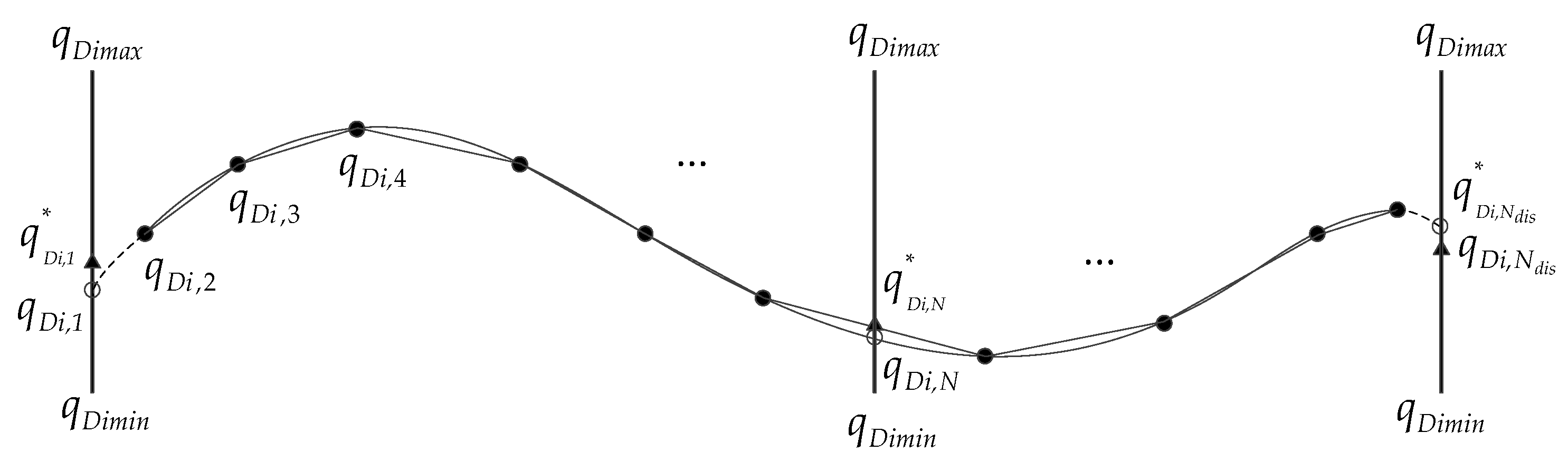
The optimization flow above can be applied to the case where there are multiple discontinuous singular positions of the path to be optimized of SITMSRS. Figure 7 elaborates the motion optimization approach in the case of non-continuous singular path points. Here, q D i , 1 * , q D i , N * , and q D i , N d i s * are true values of path initial singularity, singularity at discrete point N, and path terminal singularity, respectively.
Approximate solutions of joint angular displacements at finite intermittent singular points can be achieved by choosing the appropriate Ndis through the above approach, which reduces the complexity of path optimization at a certain level.

4.3. Solution to the Optimal Path with Discontinuous Singularity Configuration

4.3.1. Complete Path Solution Space Generation of Joints Power

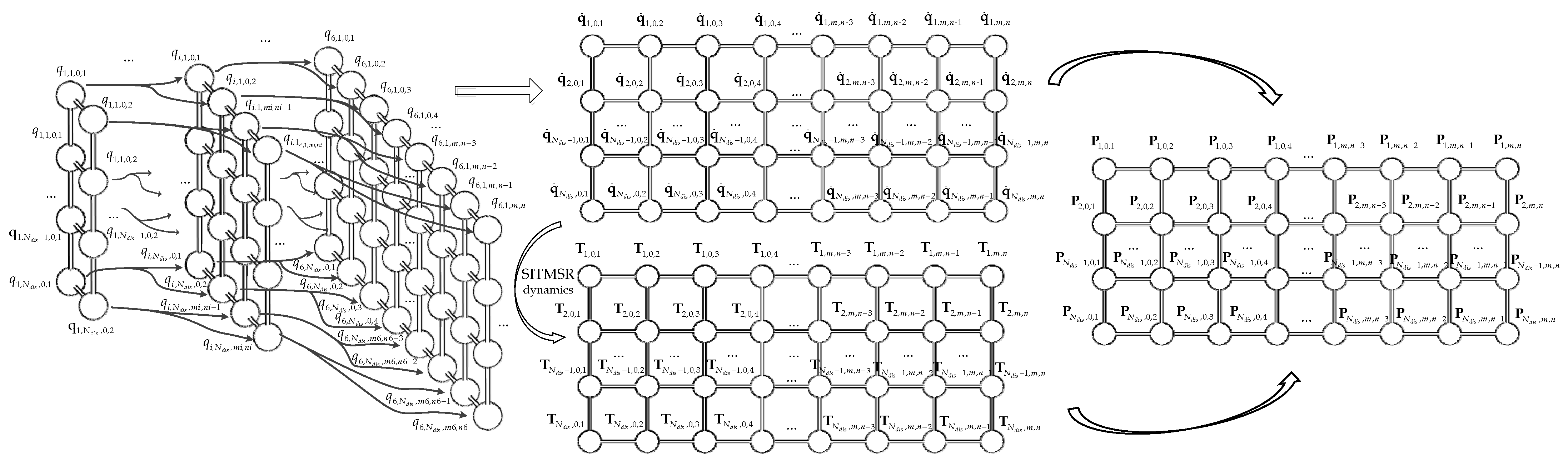
In the compound movement of each joint of SITMSR to simulate the planned motion of SIT, there are several sets of solutions at each discrete point to satisfy a given position and attitude. Complete energy consumption path solution space is needed to generate by expanding the solution of each joint at each discrete path point into a full solution matrix. Figure 8 illustrates the generation process of complete path solution space of joint power.
q i , N d i s , m i , n i and q N d i s , m , n in Figure 8 represent the (10mi+ni)-th angular displacement solution and solution vector when qi at path discrete point Ndis, respectively. T N d i s , m , n and P N d i s , m , n are the corresponding joint driving torque and joint energy consumption solution vectors, respectively. mi, ni, and P N d i s , m , n are calculated as follows:
m i = ( N i s o l n i ) / 10
n i = mod ( N i s o l , 10 )
m = max ( m i )
n = mod ( N s o l , 10 )
N s o l = max ( N i s o l )
P N d i s , m , n = ( P 1 , N d i s , m , n P 2 , N d i s , m , n P 3 , N d i s , m , n P 4 , N d i s , m , n P 5 , N d i s , m , n P 6 , N d i s , m , n ) T
where Nisol is the number of solutions of q i , j and Nsol is the maximum value of Nisol at all path discrete points of SITMSR.

4.3.2. Directed Motion Paths Construction of Energy Consumption

Constructing a networked directed non-circular motion paths of joints energy consumption of SITMSR, consisting of path nodes, directed paths, and path weights, is carried out to implement the path optimization of SITMSR on the basis of generating complete path solution space of joints power. The path node of energy consumption takes each vector of the path solution space as a node, and all nodes in the path are numbered in order. In addition, the start node and the end node are added to form a complete path to be optimized. The average of the product of the path discrete time and the sum of the energy consumption is used as the weight of the path between the two nodes except the start node and the end node. The nodes in the first row have one path weight to the initial node and Nsol path weights to other nodes. The node in row Ndis has one path weight to the destination node and Nsol path weights to other nodes. Aside from the first and last two rows, the number of input path weights and output path weights of other nodes are both Nsol. Figure 9 constructs the directed energy consumption path without continuous singularity of SITMSR.

4.3.3. Solution to Optimal Energy Consumption Path with Discontinuous Singularity

From the building of directed energy consumption path, solving the optimal path of SITMSR is searching the shortest path starting from the initial node to the end node, which meet the requirements of Equations (8) and (9). The node vectors and the corresponding weight vectors need to be established first, and then get the shortest path from the created directed motion paths through the Dijkstra algorithm. Other shortest path or second-shortest path can be achieved by repeatedly calling the Dijkstra algorithm on the basis of modifying the weight vector. The solution to the optimal path based on energy saving without continuous singularity is described as follows:
Step 1: Calculate the starting node vector S I n i from node (NdisNsol+1) to the Nsol nodes in the first row, end node vector t I n i , and corresponding path weight vector L I n i .
Step 2: Compute the starting node vector S I n i k between node k located from row one to row (Ndis − 1) and the next row of nodes, end node vector t I n i k , and weight vector L k . Here, k = 1 , 2 , , ( N d i s 1 ) N s o l .
The expression of S I n i k , t I n i k , and L k are given as follows:
S I n i k = k I 1 × N s o l
m 1 k = ( k 1 n k ) / N s o l + 1
n 1 k = mod ( k 1 , N s o l )
m 2 k = [ k ( m 1 k 1 ) N s o l n 2 k ] / 10
n 2 k = mod [ k ( m 1 k 1 ) N s o l , 10 ]
n k 1 = mod ( k , N s o l )
t I n i k = ( m 1 k N s o l + 1 , m 1 k N s o l + 2 , , ( m 1 k + 1 ) N s o l )
L k = t p 2 ( N d i s 1 ) ( | P m 1 k , m 2 k , n 2 k | I 1 × n + | ( P m 1 k + 1 , 0 , 1 , P m 1 k + 1 , 0 , 2 , , P m 1 k + 1 , m , n ) | )
In Equations (18)–(25), the definition of n 1 k is to obtain path discrete point sequence number m 1 k where the node k is located. n k 1 is introduced to get the row number and the column number of the solution vector where node k is located.
Step 3: Obtain the starting node vector S E n d from the Nsol nodes in row Ndis to node ( N d i s N s o l + 2 ) , end node vector t E n d , and corresponding path weight vector L E n d .
In Steps 1 and 3, node ( N d i s N s o l + 1 ) and node ( N d i s N s o l + 2 ) are artificially added nodes to construct the solution path to minimum energy consumption, which do not affect the solution of the optimal path. Consequently, the path weight between the initial node and the end node, and other directly connected nodes, can be set as a constant; here we take its value as 1. S I n i , t I n i , L I n i , S E n d , t E n d , and L E n d can be presented as follows:
S I n i = ( N d i s N s o l + 1 ) I 1 × N s o l
t I n i = ( 1 , 2 , , N s o l )
L I n i = L E n d = I 1 × N s o l
S E n d = [ ( N d i s 1 ) N s o l + 1 , ( N d i s 1 ) N s o l + 2 , , N d i s N s o l ]
t E n d = ( N d i s N s o l + 2 )
Step 4: Form the complete start node vector S I n t , end node vector t I n t , and weight vector L I n t of SITMSR motion path to be optimized.
Step 5: Use the Dijkstra algorithm to solve one shortest path π 1 from node ( N d i s N s o l + 1 ) to node ( N d i s N s o l + 2 ) , and acquire the node number vector O p t N o o p 1 , path weight vector L o p 1 , and path value f 2 o p 1 of π 1 .
Step 6: Traverse the path weights of other nodes except the node paths related to the initial node and the end node of π 1 in Step 5 one by one, and individually assign a new weight of + . Update the path weight vector L I n t before solving the new directional motion path and remove duplicate path solutions to achieve the vector of the node solution number, the path weight vector, and the path value of the other shortest paths.
Step 7: Reverse coding to acquire SITMSR joint angle matrix q N , m 2 k , n 2 k which corresponds to the node number vector O p t N o o p M in the shortest motion path π M ( M = 1 , 2 , ) . Determine the optimal energy consumption path by comparing the maximum joint jitter. Here it is assumed that the optimal path is π O p t , and the node number vector, the path weight vector, and the path value are O p t N o o p t , L o p t , and f 2 o p t , respectively.
The values of the objective functions can be determined through Step 7 by:
min f 2 = f 2 o p t 2
Step 8: Extract each path node except node ( N d i s N s o l + 1 ) and node ( N d i s N s o l + 2 ) of O p t N o o p t , and get the q i , j of SITMSR according to the directional motion path and the coding rules in the complete solution space and motion simulation errors by the first three constraints in Equation (9).

4.4. Solution to the Optimal Singular Path

Since the finite number of discontinuous singular points can be solved by trajectory planning, the main focus here is on the condition of the continuous singularity configuration. When SITMSR is in the singular motion path, theoretically, there are countless solutions because of the coupled motion of multi-axis motion. Singularity configuration makes it difficult to directly solve the optimal motion path based on energy saving by way of the directed node path. The reason is that when there is no singular position, the path weight between the nodes of the SITMSR path network is unique. However, there are countless path weights between the nodes at each discrete location in the singular path.
When solving the optimal energy consumption path of SITMSR with multipoint singular position and continuous singular position in given trajectory of SITS, the joint angular displacements of the singular position at the discrete point N can be set as unknown variables to be optimized. Assume that the joint angle of the coupled motion axis caused by the singularity configuration is q D i , N ( 2 D i 6 ) , and, thus, the total number of additional parameters to be optimized in the complete path solution space is N d i s D i . The constraints of q D i , N are:
q D i , N = Q 1 , N , m i , n i , Q 1 , N , m i , n i [ q D i m i n , q D i m a x ]
where Q 1 , N , m i , n i is the (10mi+ni)-th solution of q D i , N at path discrete point N.
It is hard to solve the above situation by directly using the path optimization method under the condition of non-continuous singularity position. An approximate method is to assume that the angular displacements of the coupled joints have motion constraints, and then decouple the joint motions at singular positions. The minimum energy consumption path is obtained by adjusting the coupling coefficient and using the solution algorithm for non-continuous singular configuration. The linear relationship of the coupled joints can be expressed as:
q D i , N = λ i q D 1 , N
where λ i is the coupling factors of q D i , N .
Another feasible method is to take the objective function, constraint function, and constraint function of the coupling joint as the fitness function of the intelligent optimization algorithm to solve the above problems. The problem with this method is that when Di and Ndis are small, the optimal motion path of SITMSR can be achieved. Nevertheless, the convergence process of the above optimization method is longer and the optimization fails in the case where Ndis takes a larger value. Therefore, it is necessary to improve the path optimization algorithm for the non-singular condition, so that it can handle path optimization at the SITMSR singularity configuration.
When generating the complete path solution space of energy consumption with singular positions, take the joint angle constraint relationship in Equation (32) of the coupled joint as a whole, and combine with the other uncoupled joint angle displacements to form the whole path solution space. When SITMSR is in a path with singularity, q N d i s , m , n is defined as:
q N d i s , m , n = [ q 1 , N d i s , m , n q 2 , N d i s , m , n Q 1 , N d i s , m , n 7 D i ] T
The optimal path of the uncoupled joints and the optimal path of the constraint relationship of the coupled joints π Q O p t can be acquired according to the first seven steps when optimizing with non-singular paths on the basis of generating the complete solution space of the singular path and the corresponding directional motion path on the basis of solving the optimal path of the coupling joints, which form π O p t together.
To solve the optimal motion path of each coupled joint angle, the decoupling mathematical optimization model needs to be additionally introduced for secondary optimization to gain the coupled joint angle displacements for any value of q D i , N to get the minimum value of objective function f2 under path constraints π Q O p t . It is an optimization problem with linear constraints, which can be expressed as:
min F D = t p N d i s 1 i = 1 N q N = 1 N d i s | P D i , N | ,     s . t . { q D i , N [ q D i m i n , q D i m a x ] q D i , N = Q 1 , N
where Q 1 , N is the value at the discrete point N of π Q O p t and P D i , N is the power of q D i , N .
The optimal path of each coupled joint under the singular path can be sought through applying the global optimization algorithm to decoupling the mathematical optimization model above. The optimal energy consumption trajectory of the uncoupled joint can be obtained according to Step 8 in the solution to the optimal path without singularity and the path fitting based on the polynomial difference.

5. Results

To verify the effectiveness of the proposed method, optimization solutions based on energy saving of SITMSR using KuKa KR60 programmed by Matlab introduced in previous sections are tested under different movements given in the SIT ground motion experiment. Three examples are shown in this section. The path in the first one is under the condition of discontinuous singularity configuration. Example 2 reveals the energy optimization results of coupled joints using three different solution methods under continuous singularity configuration of SITMSR. Example 3 shows the energy consumption of continuous singularity configuration and non-singularity configuration under the premise of given trajectory. The parameters and corresponding values required for examination are summarized in Table 1.

5.1. Example 1

The angular velocity of precession, nutation, and spin of SITS are φ ˙ I T 1 , θ ˙ I T 1 , and ψ ˙ I T 1 in this example, respectively. The initial value of nutation angle is −3°. In order to make full use of the robot’s reachable range of motion and to simulate the relative motion between the SIT and the aircraft operation in space as realistically as possible, the motion of OIT in SITS is set as spiral movement. Other forms of positional movement can also be set, which do not affect the verification of the proposed method. On average, the total time taken to complete the motion planning is 3.95 s in Example 1. Figure 10 shows the trajectory of SIT in the ground experiment in Example 1.
The above given trajectory is discretized by setting different values of Ndis, and the cubic polynomial is used to fit and discretize the joint paths of SITMSR. Figure 11a shows the relationship between velocity and angular velocity errors and Ndis of SITS in motion planning. Force and torque error measured by six-axis force/torque sensor between the given motion and the planned motion are given in Figure 11b.
It can be seen from the Figure 11 that when Ndis = 100, the velocity, angular velocity, force, and torque errors are 0.032 mm/s, 0.160 mm/s, 0.193 mm/s, 0.003°/s, 0.024°/s, 0.064°/s, 0.005 N, 0.026 N, 0.028 N, 4.755 × 10⁻⁴ N·m, 0.006 N·m, and 0.011 N·m, respectively, all of which meet the required motion planning accuracy.
The search algorithm based on the solution to the optimal path with discontinuous singularity configuration is used when Ndis = 100 to get O p t N o o p t and f 2 o p t of πOpt with minimum energy consumption. Here, the shortest path πSL is selected for comparison with πOpt. The path node number of πOpt and πSL and the comparison of path length with Ndis are shown in Figure 12a. The comparison of energy consumption with time are shown in Figure 12b.
As can be seen from the above curves, compared with path πSL, although the optimal path πOpt rotates 23.43% more in the joint angular displacement, its energy consumption is saved by 72.67%.
There are also differences in joints driving the torque of SITMSR on the above paths. Figure 13a,b, respectively, present the performance of joints driving the torque in the planned motion path of πOpt and πSL. The maximum joint driving the torque when the SITMSR moves along the planning path πOpt is only 63.84% of that along path πSL.
In terms of smoothness of motion, the jitter of the robot joints under the path πOpt and path πSL are shown in Figure 14a,b. The maximum jitter value of SITMSR when moving along path πSL is 0.034 rad/s3, which occurs at joint 4, while the maximum jitter value of path πOpt is 0.162 rad/s3, which also happens at joint 4. The joint jitter along the optimal path of energy consumption is, obviously, larger than that along the shortest path, which means that the joints are also subject to greater impact, but its value is within the range of the SITMSR.
The comparison results of path πOpt and path πSL in Example 1 are summarized in Table 2.

5.2. Example 2

In this example, the condition where the wrist joint of SITMSR is in continuous singularity configuration, that is, the rotation axis of robot joint four and joint six is collinear. Under the precondition that the end trajectory of SITS is given, the trajectory of other joints is determined, except for q4 and q6. Therefore, optimizing the joint space path of the coupling joint is focused to ensure optimal energy consumption. The precession angular velocity and nutation angular velocity of SITS are set as zeros and the angular velocity of spin of SITS is ψ ˙ I T 2 . The constraints of the angular displacement and the angular velocity of the coupled joints are shown in Figure 15a. The trajectory of the centroid of SITS is shown in Figure 15b.
The proposed algorithm (method 1) in the previous section is applied to optimize the energy consumption of the coupling joints in the case of continuous singularity of SITMSR. The friction torque during the motion of the coupled joint is considered, and it is assumed that it satisfies a linear relationship with the angular velocity, and the friction coefficients of q4 and q6 are C4 and C6, respectively. The convergence curve of FD with iteration is shown in Figure 16a. The average running time of motion planning based on energy saving using method 1 is 36.67 s. After the solution is completed, the trajectory of each coupled joint can be obtained, as shown in Figure 16b. It can be seen from the optimization results that when the iteration runs to Step 68, the energy consumption converges to 2.49 J, and the maximum residual error is 1.02 × 10⁻¹²°. The rotation angle of q4 is 76.89° more than that of q6.
In order to verify the effectiveness of the above solving of the algorithm, a directional path search algorithm based on the linear decoupling method is used to solve the above issue. The relationship between energy consumption and its ratio to method 1 and λ1 is shown in Figure 17a. The angular displacements of the coupled joints and energy consumption when λ1 = 1.17 are shown in Figure 17b.
In Figure 17, the energy consumption of the coupled joints decreases with the increase of λ1 until it reaches the minimum value of 3.47 J. Compared with method 1, the minimum relative increase energy consumption is 28.24%, and the value of λ1 reaches the maximum at this time. If λ1 continues to increase, it will cause the joint angular displacement to exceed the range of motion.
The genetic algorithm is adopted to solve the minimum energy consumption under the condition in Example 2. Set the initial population number of the genetic algorithm to 300, and the maximum generation to 800. Since the results of the genetic algorithm are different each time, the joint angular displacements take a set of solutions corresponding to the minimum energy consumption value. The convergence curve of energy consumption of SITMSR in the case of continuous singularity using genetic algorithm is shown in Figure 18a. The angular displacements of the coupled joint corresponding to the minimum energy consumption obtained by the genetic algorithm is shown in Figure 18b.
It can be seen from the Figure 18 that the minimum energy consumption of the genetic algorithm solution is 2.78 J, which is similar to method 1, which also verifies the effectiveness of the proposed solution method. The comparison of the results of the above three methods under the condition of continuous singularity configuration of SITMSR are summarized in Table 3.

5.3. Example 3

In this example, the given centroid trajectory of SITS is shown in Figure 18b, and its precession and nutation motion settings are the same as in Example 2, but the spin angular velocity is 0.5 times that in Example 2. The optimization method of continuous singularity of SITMSR is used to optimize the coupled joint motion, and then the directional path map of energy consumption is constructed for path optimization. Here, the non-singularity path πNs is compared with the path πOpt, which is also the energy-efficient path. The relationship between path length ratio and energy ratio of πNs and πOpt with time are shown in Figure 19.
Although the lengths of the two paths are approximately the same, the optimal path πOpt saves 6982.36 J compared to the path πNs. The comparison results of path πNs and path πOpt in Example 3 are shown in Table 4.

6. Conclusions

In this paper, a motion planning method of SITMSR based on energy saving and its corresponding joint trajectory solving algorithm are proposed. Simulations based on different given motions of SIT in the ground experiment are conducted to verify the effectiveness of presented approach. The above research mainly consists of three parts: first, the motion trajectory and accuracy requirements of SIT are mapped to the ground test system (SITMSRS); second, discrete optimization mathematical model and constraints of energy consumption of SITMSR are established; third, the Dijkstra algorithm and adding the global optimization algorithm are used to get the solutions of the SITMSR path with minimal energy consumption under the condition of discontinuous singularity configuration and continuous singularity configuration, and the trajectory of each joint is obtained through polynomial fitting and discretization of solved path.
The general form of SIT makes it difficult for ground simulation robots to avoid singular positions completely, which brings new challenges to motion planning based on energy optimization. The proposed method is based on the kinematics and dynamics of the robot, which helps to solve the problem of optimal energy consumption when manipulator exists singularity configuration under a given end trajectory. From the results in this paper, the robot consumes less energy in singularity configuration under the premise that the trajectory of the motion is satisfied. In addition, the motion planning method based on energy saving is also applicable to 7-DOF manipulators and robot systems with more DOF. The algorithm presented can obtain the global optimal solution. However, the dynamics of the robot becomes complicated with the increase of DOF, which will increase the computation amount of the proposed method and the cost of hardware implementation.
Future work will further improve the efficiency of the algorithm operation. The main work is speeding up the generation process of complete path solution space of joints power based on robot dynamics. The interface of cyber–human interaction will need to be designed and the motion planning method will need to be embedded in the real-time software of the ground semi-physical test system. High-performance computer hardware will be used to support the operation of the algorithm. In addition, joint stiffness should be considered when the proposed method is applied to a cooperative manipulator with 7-DOF or robots with more DOF. The evaluation will be carried out to quantify its impact on energy consumption in the process of robot motion planning.

Author Contributions

Conceptualization, X.B. and Z.X.; methodology, X.B. and X.L.; software, X.B. and M.L.; validation, Z.Z. (Zhang Zhang) and Z.Z. (Zhen Zhao); writing—review and editing, X.B. and M.Y.; supervision, Q.X. and X.L.; project administration, X.B. and Z.X. All authors have read and agreed to the published version of the manuscript.

Funding

This research is funded by China Manned Space Engineering Office, grant number 030501.

Institutional Review Board Statement

Not applicable.

Informed Consent Statement

Not applicable.

Data Availability Statement

The data presented in this study are available upon request from the first author. The data are not publicly available due to intellectual property protection.

Conflicts of Interest

The authors declare no conflict of interest.

References

  1. Takeichi, N.; Tachibana, N. A tethered plate satellite as a sweeper of small space debris. Acta Astronaut. 2021, 189, 429–436. [Google Scholar] [CrossRef]
  2. Sun, C.; Wan, W.; Deng, L. Adaptive space debris capture approach based on origami principle. Int. J. Adv. Robot. Syst. 2019, 16, 172988141988521. [Google Scholar] [CrossRef] [Green Version]
  3. Witze, A. The quest to conquer earth’s space junk problem. Nature 2018, 561, 24–26. [Google Scholar] [CrossRef]
  4. Shan, M.; Guo, J.; Gill, E. Review and comparison of active space debris capturing and removal methods. Prog. Aerosp. Sci. 2016, 80, 18–32. [Google Scholar] [CrossRef]
  5. Biesbroek, R.; Soares, T.; Husing, J.; Innocenti, L. The e.Deorbit cdf study: A design study for the safe removal of a large space debris. In Proceedings of the 6th European Conference on Space Debris, Darmstadt, Germany, 22–25 April 2013. [Google Scholar]
  6. Xu, W.; Liang, B.; Xu, Y.; Li, C.; Qiang, W. A ground experiment system of free-floating robot for capturing space target. J. Intell. Robot. Syst. 2007, 48, 187–208. [Google Scholar] [CrossRef]
  7. Zappulla, R.; Llop, J.V.; Park, H.; Zagaris, C.; Romano, M. Floating spacecraft simulator test bed for theexperimental testing of autonomous guidance, navigation, and control of spacecraft proximitymaneuvers and operations. In Proceedings of the AIAA/AAS Astrodynamics Specialist Conference, Long Beach, CA, USA, 13–16 September 2016. [Google Scholar]
  8. Yang, H.; Jin, M.; Xie, Z.; Sun, K.; Hong, L. Ground verification of space robot capturing the free-floating target based on visual servoing control with time delay. Ind. Robot. 2014, 41, 543–556. [Google Scholar] [CrossRef]
  9. Yang, H.; Xie, Z.; Sun, K.; Zhao, X.; Jin, M.; Li, C. Development of ground experiment system for space end-effector capturing the floating target in 3-dimensional space. Ind. Robot. Int. J. 2015, 42, 347–358. [Google Scholar] [CrossRef]
  10. Camposeco-Negrete, C.; Calderón-Nájera, J. Sustainable machining as a mean of reducing the environmental impacts related to the energy consumption of the machine tool: A case study of aisi 1045 steel machining. Int. J. Adv. Manuf. Technol. 2019, 102, 27–41. [Google Scholar] [CrossRef]
  11. Valero, F.; Mata, V.; Besa, A. Trajectory planning in workspaces with obstacles taking into account the dynamic robot behaviour. Mech. Mach. Theory 2006, 41, 525–536. [Google Scholar] [CrossRef]
  12. Garrido, J.; Yu, W.; Li, X. Robot trajectory generation using modified hidden markov model and lloyd’s algorithm in joint space. Eng. Appl. Artif. Intell. 2016, 53, 32–40. [Google Scholar] [CrossRef]
  13. Wang, H.A.; Hw, B.; Huang, J.A.; Zhao, B.A.; Quan, L.A. Smooth point-to-point trajectory planning for industrial robots with kinematical constraints based on high-order polynomial curve. Mech. Mach. Theory 2019, 139, 284–293. [Google Scholar] [CrossRef]
  14. Scalera, L.; Boscariol, P.; Carabin, G.; Vidoni, R.; Gasparetto, A. Enhancing energy efficiency of a 4-dof parallel robot through task-related analysis. Machines 2020, 8, 10. [Google Scholar] [CrossRef] [Green Version]
  15. Palmieri, G.; Scoccia, C. Motion planning and control of redundant manipulators for dynamical obstacle avoidance. Machines 2021, 9, 121. [Google Scholar] [CrossRef]
  16. Nd, A.; Me, B. Improved trajectory planning of an industrial parallel mechanism by a composite polynomial consisting of bézier curves and cubic polynomials—Sciencedirect. Mech. Mach. Theory 2019, 132, 248–263. [Google Scholar]
  17. Wang, Z.Q.; Liu, X.Q.; Wang, X.R.; Li, C.Y.; Yang, N.; Lin, T.S.; He, P. Robotic milling of complex nurbs surface with fixed cutter axis control method. Ind. Robot. Int. J. Robot. Res. Appl. 2021, 48, 413–422. [Google Scholar]
  18. Available online: https://www.sciencedirect.com/science/article/pii/S1877705816312279?via%3Dihub (accessed on 14 December 2021).
  19. Available online: https://ieeexplore.ieee.org/abstract/document/7294220 (accessed on 14 December 2021).
  20. Saeed, R.A.; Recupero, D.R.; Remagnino, P. The boundary node method for multi-robot multi-goal path planning problems. Expert Syst. 2021, 38, e12691. [Google Scholar] [CrossRef]
  21. Taghavifar, H.; Rakheja, S.; Reina, G. A novel optimal path-planning and following algorithm for wheeled robots on deformable terrains. J. Terramechanics 2020, 96, 147–157. [Google Scholar] [CrossRef]
  22. Hao, B.; Du, H.; Dai, X.; Liang, H.; Kung, H.-Y. Automatic recharging path planning for cleaning robots. Mob. Inf. Syst. 2021, 2021, 1–19. [Google Scholar] [CrossRef]
  23. Qadir, Z.; Ullah, F.; Munawar, H.S.; Al-Turjman, F. Addressing disasters in smart cities through uavs path planning and 5g communications: A systematic review. Comput. Commun. 2021, 168, 114–135. [Google Scholar] [CrossRef]
  24. Gough, E.; Conn, A.; Rossiter, J. Planning for a tight squeeze: Navigation of morphing soft robots in congested environments. IEEE Robot. Autom. Lett. 2021, 6, 4752–4757. [Google Scholar] [CrossRef]
  25. Lu, Y.A.; Tang, K.; Wang, C.Y. Collision-free and smooth joint motion planning for six-axis industrial robots by redundancy optimization. Robot. Comput. Integr. Manuf. 2021, 68, 102091. [Google Scholar] [CrossRef]
  26. Cheng, C.; Hao, X.; Li, J.; Zhang, Z.; Sun, G. Global dynamic path planning based on fusion of improved a* algorithm and dynamic window approach. Hsi-An Chiao Tung Ta Hsueh/J. Xi’an Jiaotong Univ. 2017, 51, 137–143. [Google Scholar]
  27. Energy Saving in Mechatronic Systems through Optimal Point-to-Point Trajectory Generation via Standard Primitives. Available online: https://linkspringer.fenshishang.com/chapter/10.1007/978-3-030-03320-0_3 (accessed on 14 December 2021).
  28. Mohammed, A.; Schmidt, B.; Wang, L.; Gao, L. Minimizing energy consumption for robot arm movement. Procedia CIRP 2014, 25, 400–405. [Google Scholar] [CrossRef] [Green Version]
  29. Luo, L.-P.; Yuan, C.; Yan, R.-J.; Yuan, Q.; Wu, J.; Shin, K.-S.; Han, C.-S. Trajectory planning for energy minimization of industry robotic manipulators using the lagrange interpolation method. Int. J. Precis. Eng. Manuf. 2015, 16, 911–917. [Google Scholar] [CrossRef]
  30. Carabin, G.; Scalera, L. On the trajectory planning for energy efficiency in industrial robotic systems. Robotics 2020, 9, 89. [Google Scholar] [CrossRef]
  31. Available online: https://ieeexplore.ieee.org/abstract/document/9246499 (accessed on 14 December 2021).
  32. Abbas, N.H.; Ali, F.M. Path planning of an autonomous mobile robot using enhanced bacterial foraging optimization algorithm. Al-Khwarizmi Eng. J. 2017, 12, 26–35. [Google Scholar] [CrossRef]
  33. Fang, H.C.; Ong, S.K.; Nee, A. Adaptive pass planning and optimization for robotic welding of complex joints. Adv. Manuf. 2017, 5, 93–104. [Google Scholar] [CrossRef]
  34. Guo-Chun, Z.; Ben-Xian, X.; Industrialamp. Research on robot path planning based on artificial bee colony algorithm. Autom. Instrum. 2018, 33, 43–47. [Google Scholar]
  35. Sathiya, V.; Chinnadurai, M. Evolutionary algorithms-based multi-objective optimal mobile robot trajectory planning. Robotica 2019, 37, 1363–1382. [Google Scholar] [CrossRef]
  36. Rout, A.; Bbvl, D.; Biswal, B.B. Optimal trajectory generation of an industrial welding robot with kinematic and dynamic constraints. Ind. Robot. Int. J. 2019, 47, 68–75. [Google Scholar] [CrossRef]
  37. Wang, T.; Xin, Z.; Miao, H.; Zhang, H.; Chen, Z.; Du, Y. Optimal trajectory planning of grinding robot based on improved whale optimization algorithm. Math. Probl. Eng. 2020, 2020, 1–8. [Google Scholar] [CrossRef]
  38. Available online: https://ieeexplore.ieee.org/abstract/document/6386343 (accessed on 14 December 2021).
  39. Rubio, F.; Llopis-Albert, C.; Valero, F.; Suñer, J.L. Industrial robot efficient trajectory generation without collision through the evolution of the optimal trajectory. Robot. Auton. Syst. 2016, 86, 106–112. [Google Scholar] [CrossRef] [Green Version]
  40. Nguyen-Huynh, T.C.; Sharf, I. Adaptive reactionless motion for space manipulator when capturing an unknown tumbling target. In Proceedings of the IEEE International Conference on Robotics and Automation (ICRA 2011), Shanghai, China, 9–13 May 2011. [Google Scholar]
  41. Yang, G.; Liu, Y.; Jin, M.; Liu, H. A robust and adaptive control method for flexible-joint manipulator capturing a tumbling satellite. IEEE Access 2019, 7, 159971–159985. [Google Scholar] [CrossRef]
  42. Wang, X.; Zhou, X.; Xia, Z.; Gu, X. A survey of welding robot intelligent path optimization. J. Manuf. Process. 2020, 43, 14–23. [Google Scholar] [CrossRef]
Figure 1. Motion simulation state of SIT in the ground experiment.
Machines 09 00368 g001
Figure 2. The composition of the designed SITMSRS.
Machines 09 00368 g002
Figure 3. The motion planning flowchart of the SITMSRS.
Machines 09 00368 g003
Figure 4. The definition of DH parameters and joint coordinate systems of the SITMSR.
Machines 09 00368 g004
Figure 5. The general forms of the SITMSR joint motion trajectories.
Machines 09 00368 g005
Figure 6. Optimal selection process of Ndis.
Machines 09 00368 g006
Figure 7. The motion optimization approach in the case of the non-continuous singular path points.
Machines 09 00368 g007
Figure 8. The generation process of complete path solution space of joints power.
Machines 09 00368 g008
Figure 9. Construction of directed energy consumption paths without continuous singularity of SITMSR.
Machines 09 00368 g009
Figure 10. Ground experiment motion trajectory of SIT in example 1: (a) the centroid velocity of SITS in XGS axis; and (b) the centroid velocity of SITS in YGS axis; and (c) the centroid velocity of SITS in ZGS axis; and (d) the angular velocity of SITS in XGS axis; and (e) the angular velocity of SITS in YGS axis; and (f) the angular velocity of SITS in ZGS axis.
Machines 09 00368 g010
Figure 11. Motion planning error of SITS: (a) the relationship between velocity and angular velocity errors and Ndis; and (b) force and torque error measured by six-axis force/torque sensor between the given motion and the planned motion.
Machines 09 00368 g011
Figure 12. Comparison between πOpt and πSL: (a) the path node number of πOpt and πSL and the comparison of path length with Ndis; and (b) the comparison of energy consumption with time between πOpt and πSL.
Machines 09 00368 g012
Figure 13. Joints driving the torque comparison between πOpt and πSL: (a) the performance of the joints driving the torque of SITMSR in the planned motion path of πOpt; and (b) the performance of the joints driving the torque of SITMSR in path πSL.
Machines 09 00368 g013
Figure 14. Comparison of joints jitter under πOpt and πSL: (a) the jitter of the SITMSR joints under the path πOpt; and (b) the jitter of the SITMSR joints under the path πSL.
Machines 09 00368 g014
Figure 15. Trajectory of SITS: (a) the constraints of angular displacement and angular velocity of the coupled joints; and (b) the trajectory of the centroid of SITS.
Machines 09 00368 g015
Figure 16. Results using proposed method: (a) the convergence curve of FD with iteration; and (b) the trajectory of each coupled joint of SITMSR.
Machines 09 00368 g016
Figure 17. Results using linear decoupling method: (a) the relationship between energy consumption and its ratio to method 1and λ1; and (b) the angular displacements of the coupled joints and energy consumption when λ1 = 1.17.
Machines 09 00368 g017
Figure 18. Results using genetic algorithm: (a) the convergence curve energy consumption in the case of continuous singularity; and (b) angular displacements of the coupled joint corresponding to the minimum energy consumption.
Machines 09 00368 g018
Figure 19. Construction of directed energy consumption paths without discontinuous singularity of SITMSR.
Machines 09 00368 g019
Table 1. The parameters and corresponding values required for examination.
a 1 [ m m ] a 2 [ m m ] a 3 [ m m ] d 1 [ m m ] d 4 [ m m ] α 1 [ ° ] α 3 [ ° ] α 4 [ ° ] α 5 [ ° ] γ ω [ ° / s ]
350850145815820−90−9090−900.1
γ v ( [ m m / s ] , [ ° / s ] ) G S I T S [ N ] I 7 [ k g m 2 ] N t r a j φ ˙ I T 1 [ ° / s ] θ ˙ I T 1 [ ° / s ]
(0.3, 0.1)271.26(1.17, 0.91, 1.39)10002 sin ( 1.05 t p )
ψ ˙ I T 1 [ ° / s ] ψ ˙ I T 2 [ ° / s ] γ M ( [ N ] , [ N / m ] ) C 4 [ ( N m s ) / r a d ] C 6 [ ( N m s ) / r a d ]
2(2 × 10⁻⁴) t P 3 (0.05, 0.015)0.40.2
Table 2. The comparison results of path πOpt and path πSL.
PathPath Length [°]Energy Consumption [J] | T q i , j | m a x [ N m ] | q i , j | m a x [ r a d / s 3 ]
πOpt813.65 (+23.43%)1179.24 (−72.67%)1456.40 (+36.1%)0.162 (+0.128)
πSL623.034315.392281.500.034
Table 3. The comparison of the results of the above three methods under the condition of continuous singularity configuration of SITMSR.
MethodEnergy Consumption [J]Relative Energy Consumption [%]
Global optimization algorithm2.49−28.24
Linear decoupling method3.47
Genetic algorithm2.78−19.88
Table 4. The comparison results of path πNs and path πOpt in Example 3.
PathPath Length [°]Energy Consumption [J]Relative Energy Consumption [%]
πOpt354.00 (−0.45)2740.72−62.23%
πNs354.457256.43
Publisher’s Note: MDPI stays neutral with regard to jurisdictional claims in published maps and institutional affiliations.

