Article

Influence of Sampling Frequency Ratio on Mode Mixing Alleviation Performance: A Comparative Study of Four Noise-Assisted Empirical Mode Decomposition Algorithms

1
Department of Traffic Engineering, Huaiyin Institute of Technology, Huai’an 223003, China
2
Laboratoire de Conception, Optimisation et Modélisation des Systèmes, Université de Lorraine, 57078 Metz, France
*
Author to whom correspondence should be addressed.
Machines 2021, 9(12), 315; https://doi.org/10.3390/machines9120315
Submission received: 2 November 2021 / Revised: 20 November 2021 / Accepted: 23 November 2021 / Published: 26 November 2021
(This article belongs to the Special Issue Advances in Tool Life Prediction in Machining)

Abstract

:
Four noise-assisted empirical mode decomposition (EMD) algorithms, i.e., ensemble EMD (EEMD), complementary ensemble EMD (CEEMD), complete ensemble EMD with adaptive noise (CEEMDAN), and improved complete ensemble EMD with adaptive noise (ICEEMDAN), are noticeable improvements to EMD, aimed at alleviating mode mixing. However, the sampling frequency ratio (SFR), i.e., the ratio between the sampling frequency and the maximum signal frequency, may significantly impact their mode mixing alleviation performance. Aimed at this issue, we investigated and compared the influence of the SFR on the mode mixing alleviation performance of these four noise-assisted EMD algorithms. The results show that for a given signal, (1) SFR has an aperiodic influence on the mode mixing alleviation performance of four noise-assisted EMD algorithms, (2) a careful selection of SFRs can significantly improve the mode mixing alleviation performance and avoid decomposition instability, and (3) ICEEMDAN has the best mode mixing alleviation performance at the optimal SFR among the four noise-assisted EMD algorithms. The applications include, for instance, tool wear monitoring in machining as well as fault diagnosis and prognosis of complex systems that rely on signal decomposition to extract the components corresponding to specific behaviors.

1. Introduction

Usually, wear monitoring and fault diagnosis of complex systems rely on decomposing signals to extract the components that correspond to specific behaviors, such as abnormal phenomena or failures. These abnormal phenomena or failures express particular frequencies that are different from the standard frequencies. Up to now, researchers have presented some signal decomposition algorithms, e.g., empirical mode decomposition (EMD) and noise-assisted EMD algorithms, for identifying abnormal phenomena or failures [1]. Although EMD can adaptively process non-linear and non-stationary signals, it suffers from mode mixing [2]. Four noise-assisted EMD algorithms, i.e., ensemble EMD (EEMD), complementary ensemble EMD (CEEMD), complete ensemble EMD with adaptive noise (CEEMDAN), and improved complete ensemble EMD with adaptive noise (ICEEMDAN), are noticeable improvements to EMD, aimed at alleviating mode mixing. However, the sampling frequency ratio (SFR), i.e., the ratio between the sampling frequency and the maximum signal frequency, may significantly affect the mode mixing alleviation performance of these four noise-assisted EMD algorithms. To design a tool wear monitoring or fault diagnosis method based on a noise-assisted EMD algorithm and choose an optimal SFR, one needs to analyze and compare the influence of SFR on the mode mixing alleviation performance of these four noise-assisted EMD algorithms.
The abovementioned four noise-assisted EMD algorithms have different properties in signal decomposition. EEMD relies on adding white noise with finite amplitude to the original signal [3]. To reduce the modes’ noise caused by adding white noise, EEMD defines the mean of corresponding intrinsic mode functions (IMFs) obtained in some trials as the final IMFs. With the help of adding white noise, EEMD alleviates the mode mixing significantly. However, EEMD also involves some issues: (1) optimal selection both of the noise amplitude and the number of ensemble trials; (2) the presence of residual noise in the reconstruction signal; (3) possible generation of different numbers of modes in different trials; (4) the presence of the residual noise in modes.
For the first issue, if the amplitude of the additive noise is too small to change the extrema distribution of the original signal, the mode mixing will not be addressed. However, a high amplitude noise increases the number of ensemble trials, and thus the computational cost increases. For this issue, Wu and Huang [3] suggested setting the noise’s amplitude value to 0.2 and the number of ensemble trials to a few hundred, in most cases.
To address the second issue of EEMD, Yeh et al. [4] proposed the CEEMD algorithm, which accurately removes the residual noise in the reconstruction signal and does not result in more computational costs than EEMD. Therefore, the authors recommended CEEMD as the standard form of EEMD [4].
To solve the second and the third issues mentioned above, Torres and Colominas et al. [5,6] introduced the CEEMDAN algorithm for complete signal decomposition. A particular noise is added to extracting modes with a unique residue. Although CEEMDAN overcomes the second and third issues of EEMD, it usually produces “spurious” modes (i.e., IMFs without the original signal information) at the early decomposition stage [7].
To address the last three issues of EEMD and improve CEEMDAN, Colominas et al. [7] suggested the ICEEMDAN algorithm. During the decomposing process of ICEEMDAN, IMFs of white noise extracted by EMD are added to the original signal or the unique residue at each decomposition stage. ICEEMDAN reduces the residual noise contained in modes and the final residue. It also avoids the presence of “spurious” modes at the early decomposition stage. Table 1 summarises the essential properties of the four noise-assisted EMD algorithms.
Some researchers have compared the decomposition performance of the four noise-assisted EMD algorithms mentioned above in different research fields, such as disease diagnosis, denoising and filtering, fault diagnosis, and forecasting. In [7], the authors investigated the residual noises in modes and the capability of recovering known components in EEMD, CEEMD, CEEMDAN, and ICEEMDAN using two artificial signals and three biomedical signals. The results showed that ICEEMDAN has the best decomposition performance. Seismic data were processed in [8], where the authors demonstrated that the ICEEMDAN-based approach is a more suitable filtering method than the CEEMDAN-based method for removing high-oscillating components. In the bearing fault diagnosis field, ICEEMDAN showed higher diagnosis ability than EEMD [9]. Ren et al. [10] compared some combinations of EMD-based (EMD, EEMD, CEEMD, and CEEMDAN) algorithms, the artificial neural network, and the support vector regression (SVM), for forecasting wind speed time series. CEEMDAN-SVM showed the best performance concerning the CPU time and the number of decomposed subseries. Liu et al. [1] tested and compared the decomposition accuracy of EMD, EEMD, CEEMD, and ICEEMDAN using an artificial signal. They found that ICEEMDAN yields fewer errors compared to the other algorithms. In addition, the authors concluded that a higher sampling frequency is welcome in the process both of EMD and EEMD. This conclusion is inaccurate because the higher sampling frequency may generate poor decomposition results for EEMD [11]. Sharma et al. [12] decomposed a speech signal using the abovementioned four noise-assisted EMD algorithms. They showed that there is no significant advantage of any method over the others. This conclusion may not be accurate, since the authors did not consider the influence of SFR on the mode mixing alleviation performance of the four noise-assisted EMD algorithms.
A study on the alleviating performance of the mode mixing caused by intermittent wave components has a significant practical interest. According to [13], one can treat the intermittent wave component as a special case of amplitude-modulation (AM) signal, with zero as minimum amplitude. In the EMD decomposition process, the intermittent wave component does not contribute to extrema when its amplitude is zero. Therefore, the intermittent wave component cannot be separated from the slow-oscillating wave. Wu and Huang [3] illustrated the intermittent wave component riding on a slow-oscillating wave to show the mode mixing problem. In the fields of natural science and engineering science, the intermittent wave component is a common phenomenon. Intermittent wave components are often produced by intermittent phenomena due to cutting tool wear in a milling process, bearing and gear faults in mechanical systems, or circuit faults in electrical systems [14,15]. In the milling process, the intermittent cutting process produces intermittent wave components. In [16,17,18,19], EEMD, CEEMD, CEEMDAN, and ICEEMDAN were used to decompose the machining signal and alleviate the mode mixing caused by intermittent wave components for monitoring the tool wear state. Nevertheless, these works do not consider the influence of SFR on the mode mixing alleviation performance of the four noise-assisted EMD algorithms.
SFR may affect the mode mixing alleviation performance of the four noise-assisted EMD algorithms significantly. In [20], we investigated the influence of SFR on the mode mixing alleviation performance of the ICEEMDAN algorithm. Under the condition of the particular SFR, the decomposition instability phenomenon is observed in ICEEMDAN. Chen et al. [11] investigated the influence of SFR on the decomposition performance of the EEMD using the gearbox vibration signal. They suggested diagnosing the bearing faults using an SFR between 10.3 and 11. Therefore, one can see that SFR may affect the mode mixing alleviation performance of the four noise-assisted EMD algorithms, especially for ICEEMDAN, due to the appearance of the decomposition instability phenomenon.
In practice, to apply the four noise-assisted EMD algorithms optimally, researchers or engineers should consider the mode mixing alleviation performance under different conditions of SFR. The four noise-assisted EMD algorithms have different mode mixing alleviation performance, and SFR may affect their mode mixing alleviation performance. Therefore, it is necessary to analyze and compare the mode mixing alleviation performance of the four noise-assisted EMD algorithms for their applications, such as designing a noise-assisted EMD algorithm-based tool wear monitoring method.
To the best of our knowledge, no existing works compare the mode mixing alleviation performance of the four noise-assisted EMD algorithms regarding decomposing the signal with intermittent wave components under the condition of different SFRs.
Aimed at this gap, we investigated and compared the influence of SFR on the mode mixing alleviation performance of four noise-assisted EMD algorithms. In the case study, the mode mixing phenomenon is caused by intermittent wave components. The results are helpful for researchers or engineers processing non-linear and non-stationary signals. The major contributions are (1) the benchmarking study of the SFR influence on the mode mixing alleviation performance of four noise-assisted EMD methods, and (2) the ICEEMDAN with the optimal SFR is suggested for alleviating mode mixing.
To compare the four noise-assisted EMD algorithms fairly, we had to set their parameters consistently. According to results in [3,4,5,7], we adopted the following setting for these algorithms. For EEMD, CEEMDAN, and ICEEMDAN, the amplitude of the white noise was set to 0.2, and the number of ensemble trials was 100. For CEEMD, the amplitude of the white noise was also set to 0.2. However, the number of ensemble trails was set to 50 because there are twice the decomposition procedures in each trial [4]. The number of iterations for the four algorithms was 10. Numerical simulations were conducted using Matlab 2016a.
The rest of this paper is organized as follows. Section 2 briefly introduces EMD, EEMD, CEEMD, CEEMDAN, and ICEEMDAN. Section 3 shows a metric for assessing the mode mixing alleviation performance. Section 4 is devoted to analyzing and comparing the influence of SFR on the mode mixing alleviation performance of the four noise-assisted EMD algorithms. The last section concludes this paper.

2. Materials and Methods

2.1. Notations

To describe EMD and the four noise-assisted EMD algorithms conveniently, we summarized the related parameters according to corresponding algorithms in Table 2.

2.2. EMD

The EMD algorithm decomposes the non-linear and non-stationary signal into a set of IMFs adaptively. However, the mode mixing phenomenon may appear in the decomposition process when the decomposed signal contains intermittent components [2].
EMD is a well-known signal processing method. Studies on this algorithm can be found in large amounts in the literature [2]. In addition, its Matlab code is available online. Thus, we will not illustrate the EMD algorithm in detail.
To illustrate the mode mixing phenomenon caused by intermittent components, we considered the first two components of the simulated signal used in [4]. Therefore, the simulated signal used in this paper, denoted x ( t ) , is composed of an intermittent signal x 1 ( t ) and a sinusoidal signal x 2 ( t ) . The intermittent component is a sinusoidal signal with amplitude α 1 and frequency f 1 , which appears at some durations. The sinusoidal component is a sinusoidal signal with amplitude α 2 and frequency f 2 . Two components and the signal x ( t ) are given as follows:
x 1 ( t ) = { α 1 sin ( 2 π f 1 ( t 1.88 ) ) 1.88 t 2.12 α 1 sin ( 2 π f 1 ( t 8.38 ) ) 8.38 t 8.62 α 1 sin ( 2 π f 1 ( t 11.88 ) ) 11.88 t 12.12 α 1 sin ( 2 π f 1 ( t 17.88 ) ) 17.88 t 18.12 0 o t h e r s
x 2 ( t ) = α 2 sin ( 2 π f 2 t + π 2 )
x ( t ) = x 1 ( t ) + x 2 ( t )
To introduce the algorithms conveniently, we consider the digitalized signal in the rest of the paper. Figure 1 shows the digital signal and its components, with a particular set of parameters. The amplitudes of the two components are 0.05 and 1. Thus, the amplitude ratio (AR), i.e., the ratio between amplitudes of intermittent and sinusoidal components, is 0.05. The frequencies of the two components are 85 Hz and 10 Hz. The sampling frequency is set to 200 Hz, and so the SFR equals 2.35. The abscissa represents the number of sampling points, k = t T , where T is the sampling period. The ordinate represents the digital signal values x ( k ) , x 1 ( k ) and x 2 ( k ) at each sampling point k.
Figure 2a shows the decomposition results of the signal x ( k ) using EMD. The components x 1 ( k ) and x 2 ( k ) contained in the original signal x ( k ) are decomposed into the first two IMFs (i.e., IMF1 and IMF2) with severe mode mixing. The real meaning of the individual IMF is unclear. Thus, we can find that the mode mixing reduces the decomposition performance of EMD significantly.

2.3. EEMD

Wu and Huang [3] developed the EEMD algorithm to address the mode mixing issue. This algorithm is a noise-assisted decomposition algorithm that adds white noise with finite amplitude to the original signal. The added white noise changes the extrema distribution of the original signal. Therefore, the intrinsic local oscillations are filtered to the proper scales, and thus the mode mixing is alleviated. However, the decomposition results are noisy due to the addition of white noise. Fortunately, the ensemble process can reduce the noise embedded in the decomposition results. The EEMD algorithm yields satisfactory results by conducting, using the algorithm in Appendix A, several successive decompositions of the original digital signal x ( k ) , which can be expressed as
x ( k ) = i = 1 n c i ( k ) + r n ( k )
where n is the number of IMFs, c i is the ith IMF, and r n ( k ) represents the final residual, also called the reconstruction error (see the detailed algorithm in Appendix A).
Figure 2b depicts the EEMD decomposition results of the signal x ( k ) . We can see that EEMD alleviates the mode mixing in the first two modes (IMF1 and IMF2) distinctly. However, for some signals containing large-amplitude intermittent components, EEMD cannot perfectly decompose them under the condition of a specific SFR. For instance, Figure 3a shows the decomposition results of EEMD for the signal x ( k ) with the AR of 0.3. The mode mixing occurs again in IMF1, IMF2, and IMF3 (see the green box).
The results illustrate that EEMD cannot alleviate the mode mixing at the SFR of 2.36 when the digital signal’s AR is relatively high. Section 3 will further discuss this issue. The reason may be that, at a specific SFR, the added white noise does not sufficiently change the extrema distribution of the signal with the relatively large AR. To decompose precisely the signal with large AR, one should use a suitable SFR or the white noise with large amplitude in the decomposition process using EEMD.

2.4. CEEMD

EEMD alleviates the mode mixing significantly. However, it involves the issue of the reconstruction error. Yeh et al. [4] developed the CEEMD algorithm to reduce this reconstruction error, which adds pairs of white noise (i.e., positive and negative white noise) to the original signal. Thus, two mixtures containing the original signal and white noise are composed as follows:
[ x m + ( k ) x m ( k ) ] = [ 1 1 1 1 ] [ x ( k ) β ω m ( k ) ] ,
where x m + ( k ) and x m ( k ) represent two mixed signals at the mth trial.
The decomposition procedure of CEEMD is similar to the one of EEMD. The final IMF c i ( k ) is obtained by calculating the mean of the ith IMF in M/2 trials:
c i ( k ) = 1 M m = 1 M / 2 ( c i + m ( k ) + c i m ( k ) ) ,
where c i + m ( k ) and c i m ( k ) denote the ith IMF decomposed at mth trial (m = 1, 2, 3, …, M/2), obtained from two mixed signals with positive and negative noises, respectively.
CEEMD removes the reconstruction error practically, while the computation effort is similar to EEMD. Therefore, the authors recommend it as the standard form of EEMD [4]. However, IMFs decomposed by CEEMD still contain some noises, and a different number of IMFs may occur at different trials [7].

2.5. CEEMDAN

Different numbers of IMFs may occur at different trials for EEMD or CEEMD. This issue will lead to challenging work for the final averaging of IMFs obtained in all trials [5,6]. To address this issue, Torres et al. [5] proposed an extension of the EEMD algorithm, called CEEMDAN. This algorithm obtains the first mode using the same procedure as EEMD. The other modes are obtained by combining a unique residue with particular noises produced by EMD. CEEMDAN allows for avoiding conflicts of the final averaging. Appendix B describes the CEEMDAN algorithm.
CEEMDAN solves the issue arising from the different numbers of IMFs at different trials. However, new issues arise in CEEMDAN. Some ‘spurious’ modes (see the dashed line red box in Figure 3c) appear earlier than ones containing signal information [7].

2.6. ICEEMDAN

To suppress the CEEMDAN issue mentioned above and the EEMD issues, Colominas et al. [7] proposed the improved CEEMDAN (ICEEMDAN), based on the work of [5]. ICEEMDAN uses particular noises, which are extracted from the white noise, at each decomposition stage (see the detailed algorithm in Appendix C).
Figure 3d displays the decomposition results of ICEEMDAN. Two components are decomposed into IMF1 and IMF2 accurately. ICEEMDAN obtains perfect decomposition results.

3. Metric

Four noise-assisted EMD algorithms were implemented to decompose the signals embedding the intermittent components with different magnitudes. We used the decomposition results to evaluate and compare the influence of SFR on the mode mixing alleviation performance of four noise-assisted EMD algorithms. To this end, we proposed using the relative root squared error (RRSE). RRSE is defined as follows:
RRSE = a ( k ) b ( k ) a ( k ) ,
where the reference a ( k ) corresponds to the intermittent signal x 1 ( k ) or the sinusoidal signal x 2 ( k ) according to the analyzed component, the obtained IMF yields the recovered signal b ( k ) , i.e., the closest IMF to the reference a ( k ) .
The RRSE is used to evaluate and compare the influence of SFR on the mode mixing alleviation performance of the four noise-assisted EMD algorithms. The RRSE measures the relative decomposition error of the extracted component. If RRSE is small or close to zero, the corresponding IMF is close to the original component, and the mode mixing alleviation performance is high, and vice versa.

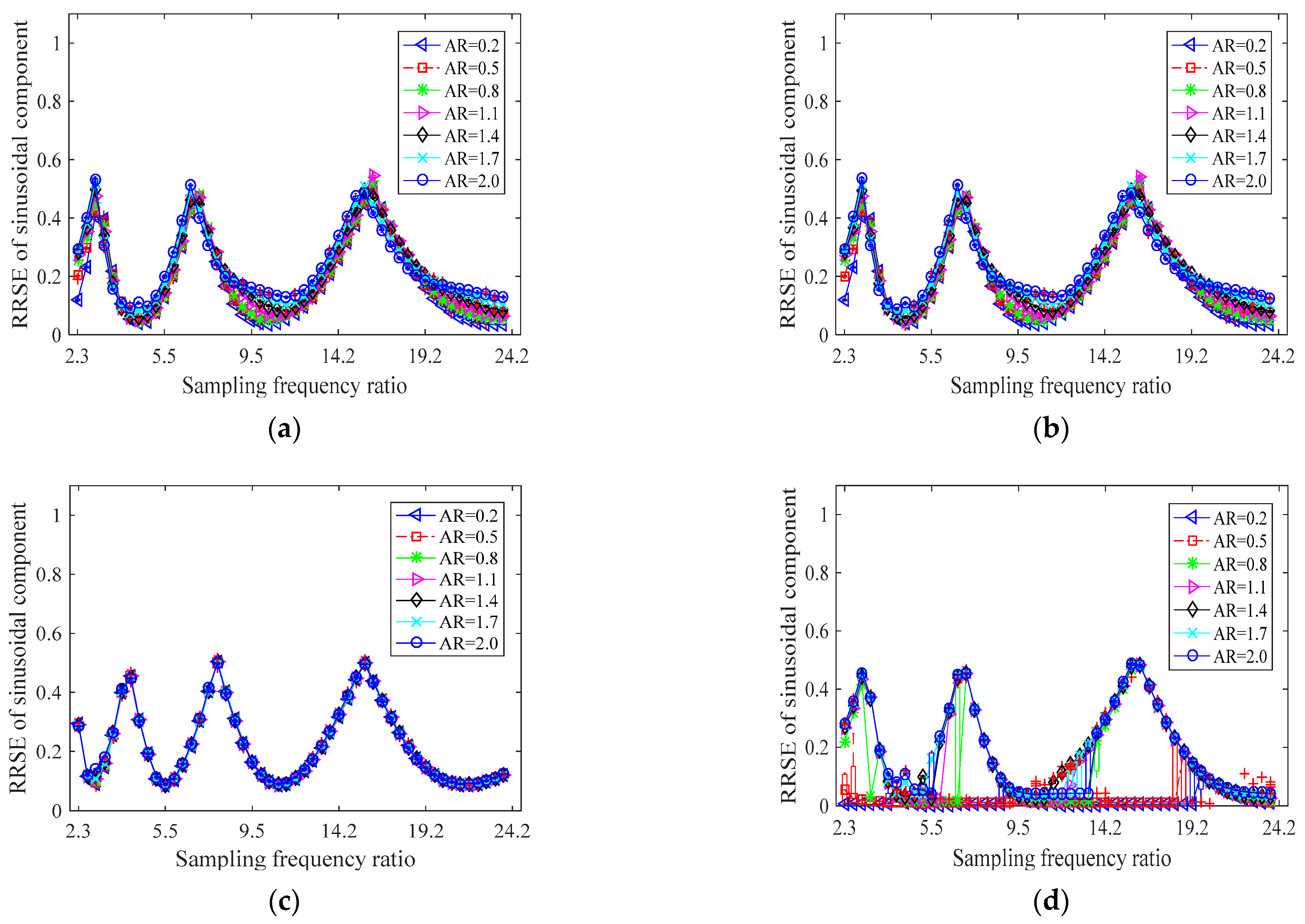
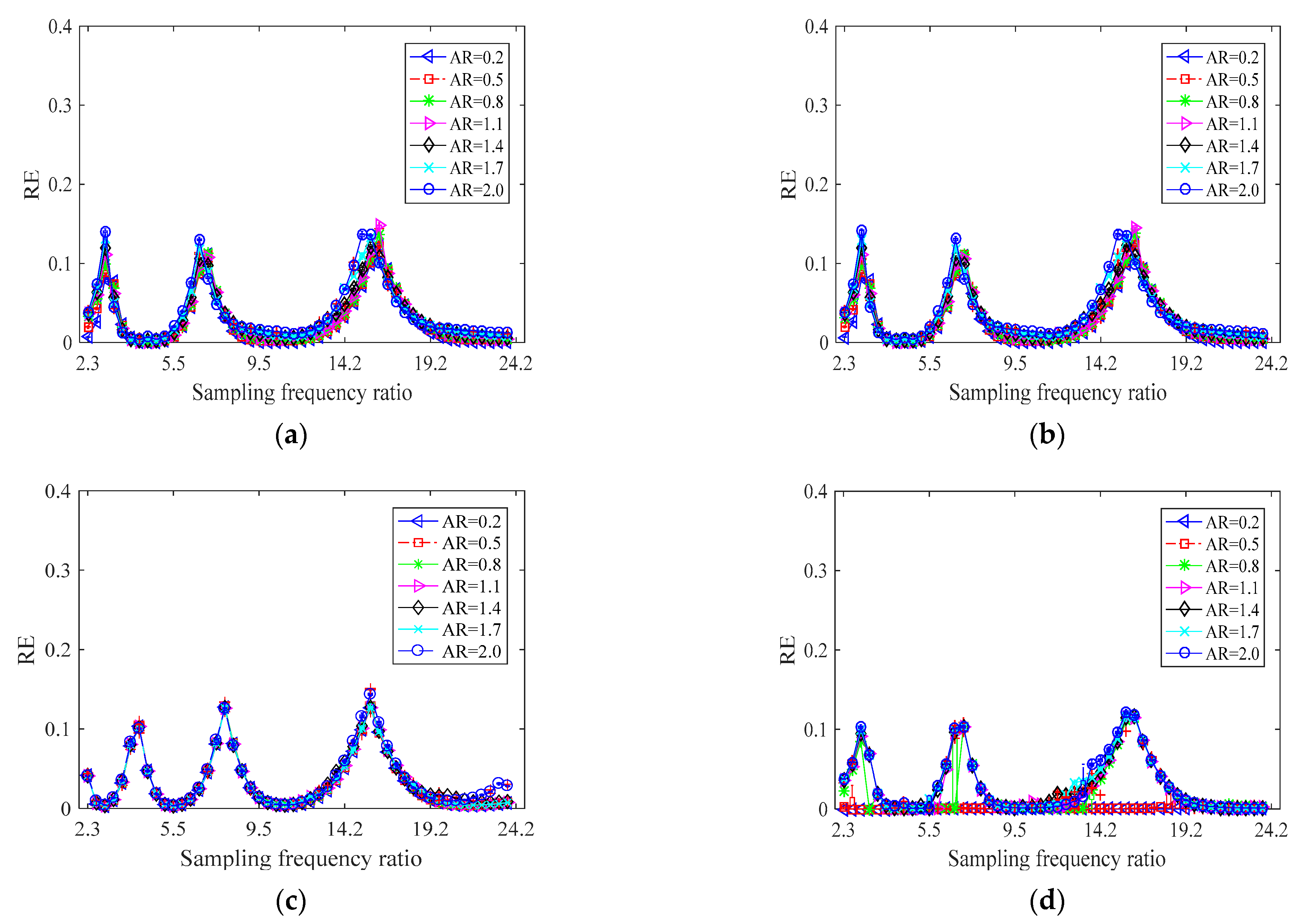
4. Comparative Results and Discussion

To illustrate and compare the influence of the SFR on the mode mixing alleviation performance of four noise-assisted EMD algorithms, we consider the benchmark signal given in Section 2.2. This kind of signal appears in practice frequently.
Numerical experiments were conducted considering an AR from 0.2 to 2.0, with the increasing step 0.3 and a series SFR ranking of 2.3 to 24.2 with variable steps. According to the Nyquist-Shannon sampling theorem, a signal can be reconstructed when the sampling frequency is more than twice the maximum signal frequency. Therefore, we set the minimum sampling frequency equal to 2.3 times the maximum signal frequency, i.e., the SFR equals 2.3. However, a high SFR will lead to a high computational cost. Thus, we considered the range of SFR from 2.3 to 24.2 in these comparative experiments. To check decomposition stability, we conducted every numerical experiment 20 times.
The following contents are illustrative of the influence of the SFR on the mode mixing alleviation performance of the four noise-assisted EMD algorithms.
Figure 4a–d displays the RRSE of the intermittent component, i.e., the first component embedded in the original signal, for the four noise-assisted EMD algorithms at different ARs and SFRs. The SFR influences the RRSE of the intermittent component dramatically. For different ARs, the influence of the SFR on RRSE of the four noise-assisted EMD algorithms is different. Even so, these RRSEs have similar fluctuations. They vary quasi-periodically with the increase of the SFR. Some RRSE values are very close to zero. This means that the extraction precision of the intermittent component is perfect under the condition of these SFRs. Therefore, an appropriate SFR can significantly improve the extraction precision of the intermittent component from a signal characterized by a given AR. In addition, the local minimum RRSE values increase slightly with the SFR.
The decomposition instability phenomenon appears in the four noise-assisted EMD algorithms at the AR of 0.5. The decomposition instability means that both good and poor decomposition results are obtained for the same setting. We also observed the decomposition instability phenomenon in CEEMD and ICEEMDAN at the AR of 0.8.
From the above results, we can see that increasing the SFR may not improve the mode mixing alleviation performance of the four noise-assisted EMD algorithms. This conclusion is different from that in [1]. For EEMD, a higher SFR may not be useful for decomposing the signal with an intermittent component. To extract a more accurate intermittent component stably, we should set an appropriate SFR value according to the AR value.
Figure 5a–d illustrates the RRSE of the sinusoidal component of the original signal for the four noise-assisted EMD algorithms. The results show that SFR also influences the extraction precision of the sinusoidal component at all ARs. The RRSE of the sinusoidal component varies quasi-periodically with the increase of the SFR for the four noise-assisted EMD algorithms. An appropriate SFR value can also significantly improve the extraction of the sinusoidal component from a signal characterized by a given AR. In other words, a reasonable SFR value significantly improves the mode mixing alleviation performance for the four noise-assisted EMD algorithms.
EEMD and CEEMD have similar extraction precision of the sinusoidal component. These two noise-assisted EMD algorithms have similar decomposition processes. EEMD uses the general white noise, while CEEMD adopts negative and positive white noise in couples. Although the used white noises are not the same, their statistical properties are the same. The AR also influences the extraction precision of the sinusoidal component in some ranges of SFR. The extraction precision of the sinusoidal component decreases with the increase of the AR.
For CEEMDAN, the AR does not affect the extraction precision of the sinusoidal component. However, for ICEEMDAN, the AR influences the extraction precision of the sinusoidal component significantly. The extraction precision of the sinusoidal component degrades with the increase of the AR. In some ranges of SFR, the RRSE of the sinusoidal component is close to zero. This means the sinusoidal component can be extracted perfectly. Nevertheless, these ranges decrease with the increase of AR. Decreasing these ranges of SFR implies that the selectable SFR range for obtaining optimal extraction results decreases. Among the four noise-assisted EMD algorithms, ICEEMDAN obtains the best extraction precision of the sinusoidal component by choosing the optimal SFR.
The decomposition instability is observed for several SFR values in the extraction process of the sinusoidal component by using EEMD, CEEMD, and ICEEMDAN. We did not find the decomposition instability phenomenon in the decomposition process of CEEMDAN. The decomposition instability is severe in ICEEMDAN. To obtain the optimal mode mixing alleviation performance, we should avoid the decomposition instability by choosing SFR, especially for ICEEMDAN.
In practice, it is not enough to select an appropriate SFR for some applications according to the mode mixing alleviation performance of the four noise-assisted EMD algorithms because their other decomposition performances are also critical. For instance, designing a fault diagnosis method based on a noise-assisted EMD algorithm needs to consider the decomposition performance thoroughly. Although the mode mixing alleviation performance reflects the decomposition performance, the other decomposition performances need to be analyzed further by using some indicators such as residual energy (RE) and successive IMF orthogonality (SIO) [11,21]. The RE is the energy of unexpected modes and indicates the leakage energy of decomposition. The SIO evaluates the orthogonality of noise-assisted EMD algorithms. Less RE and SIO imply better decomposition performance and vice versa.
Figure 6 and Figure 7 illustrate the RE and SIO of the four noise-assisted EMD methods, respectively. The results show that the SFR has a similar influence on the RE and SIO as the RRSE of the sinusoidal component. The RE and SIO also vary quasi-periodically with the increase of SFR for EEMD, CEEMD, and CEEMDAN. In addition, one can notice that the decomposing results of EEMD and CEEMD show similar trends as SFR.
For ICEEMDAN, the RE and SIO are very close to 0 when the AR is 0.2. It means that ICEEMDAN has the perfect decomposition results in all SFR ranges. When the AR increases up to 0.5 or 0.8, the decomposition performance degrades in some ranges of SFR, e.g., when SFR = 10.3 to 14. The decomposition performance decreases with the increase of AR. Nevertheless, under the condition of the worst decomposition performance of ICEEMDAN, it has similar results with the other three algorithms in these SFR ranges. In other words, ICEEMDAN can obtain the best decomposition performance among the four noise-assisted EMD algorithms by choosing an appropriate SFR.
ICEEMDAN produces a more severe decomposition instability phenomenon than the other three noise-assisted EMD algorithms. Table 3 displays the decomposition results of ICEEMDAN in 20 simulations with the same setting. For 12 simulations (results displayed with bold characters), the decomposition performance is excellent, while it is terrible for the other eight simulations. The noise used in ICEEMDAN is obtained from white noise through EMD decomposition. The randomness of the used noise can explain the decomposition instability. This noise may not be enough to change the extrema distribution of the original signal at some decomposition processes.
It is worth noting that Sharma et al. [12] compared the decomposition performance of the four noise-assisted EMD algorithms using speech signals. They selected a specific sampling frequency of 8k Hz and found no significant advantage of any algorithm over the others. Unlike the results in [12], we showed that the decomposition performance of the four noise-assisted EMD algorithms is not the same. ICEEMDAN has the best decomposition performance for the signal with intermittent components. According to the signal characteristics, there is a significant advantage of an appropriate choice of both the noise-assisted EMD algorithm and SFR.
To sum up, compared to the other three noise-assisted EMD algorithms, ICEEMDAN has the best mode mixing alleviation performance, even if decomposition instability might appear in some ranges of SFR. SFR dramatically affects the mode mixing alleviation performance of the four noise-assisted EMD algorithms. Thus, to alleviate the mode mixing caused by the intermittent component and obtain relatively high decomposition performance, we propose to use ICEEMDAN for signal decomposition and to choose an appropriate SFR for data acquisition based on the signal.
It should be noted that one should conduct the decomposition process several times to consider the decomposition instability.

5. Conclusions

The research work presented in this paper focused on benchmarking the mode mixing alleviation performance of four noise-assisted EMD decomposition algorithms of a specific signal containing intermittent and sinusoidal wave components. This class of signals frequently appears in electrical and mechanical processes such as machining. The SFR and simulation-based benchmarking results allowed deriving the following observations:
(1)
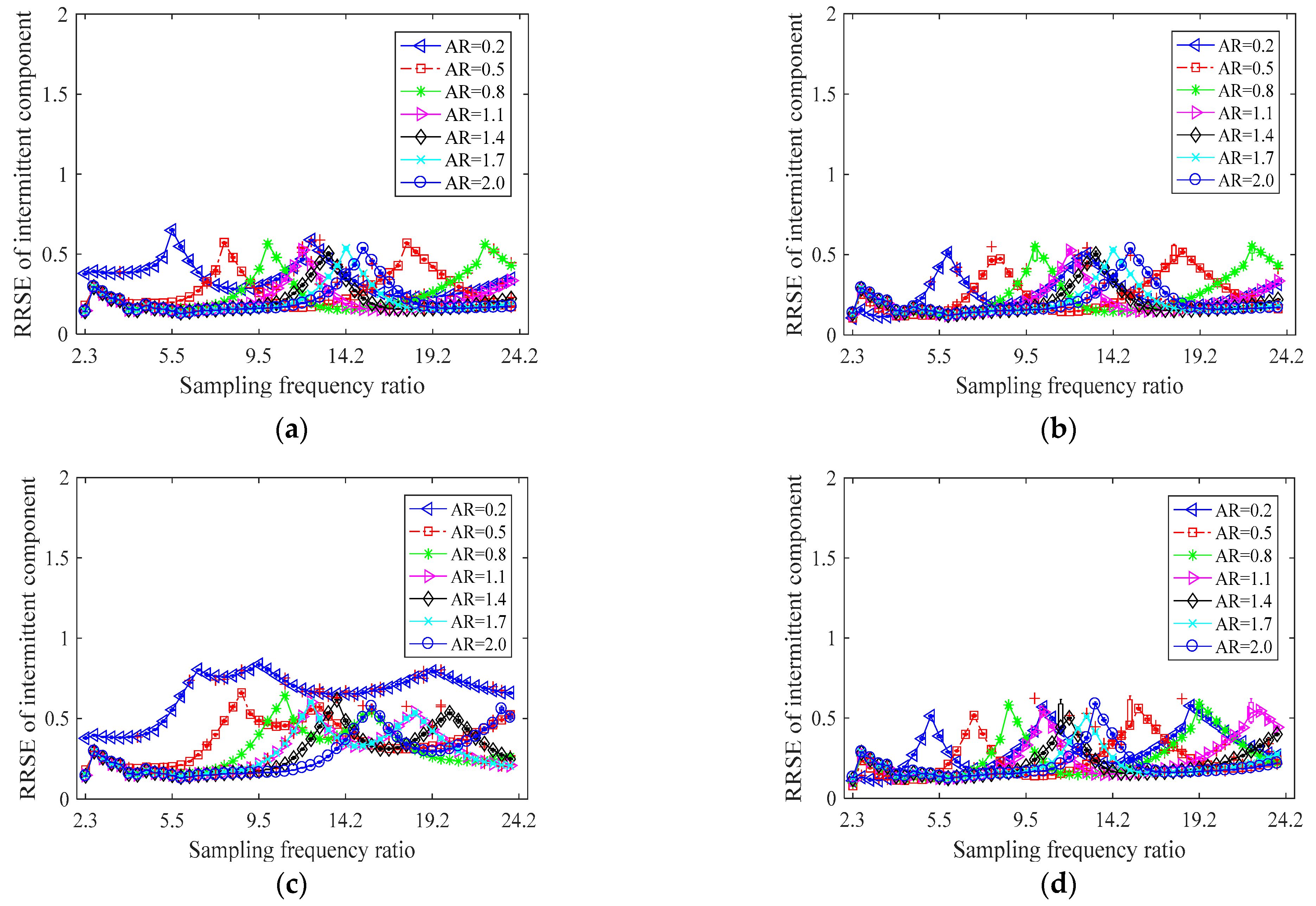
The SFR affects the mode mixing alleviation performance of the four noise-assisted EMD algorithms significantly.
(2)
The decomposition instability phenomenon appears in the four noise-assisted EMD algorithms, especially in ICEEMDAN.
(3)
ICEEMDAN has the best mode mixing alleviation performance for decomposing the signal with an intermittent component among the four noise-assisted EMD algorithms.
(4)
Selecting an appropriate SFR can improve the mode mixing alleviation performance of the four noise-assisted EMD algorithms.
An appropriate choice of the noise-assisted EMD algorithm and a careful selection of the SFR can significantly improve the decomposition of a given signal with the intermittent component. The applications include tool wear monitoring in machining systems, fault diagnosis and prognosis of complex mechanical and electrical systems, acoustic vibration signal analysis, speech signal analysis, etc., which rely on signal decomposition to extract the components corresponding to specific behaviors.
Selecting an appropriate SFR for the four noise-assisted EMD algorithms is necessary to decompose the signal processes from complex processes, such as milling and drilling tool wear, gearing and bearing faults, electrical circuits faults, etc. Moreover, selecting an appropriate SFR would strengthen the noise-assisted EMD algorithm-based fault detection and diagnosis methods. The next step in future investigations will focus on the noise-assisted EMD algorithm to monitor cutting tool wear and to detect chatter in the milling process. We believe that the optimal SFR selection is a promising research direction for improving the mode mixing alleviation performance of the four noise-assisted EMD algorithms for decomposing signals with an intermittent component.

Author Contributions

Conceptualization, Y.Z., K.H.A. and A.S.; methodology, Y.Z., K.H.A. and A.S.; numerical experiments, Y.Z.; validation, Y.Z., K.H.A. and A.S.; formal analysis, Y.Z., K.H.A. and A.S.; investigation, Y.Z., K.H.A. and A.S.; resources, Y.Z.; data curation, Y.Z. and Z.W.; writing—original draft preparation, Y.Z., K.H.A. and A.S.; writing—review and editing, Y.Z., K.H.A. and A.S.; visualization, Y.Z., K.H.A. and A.S.; supervision, K.H.A. and A.S. All authors have read and agreed to the published version of the manuscript.

Funding

This research received no external funding.

Institutional Review Board Statement

Not applicable.

Informed Consent Statement

Not applicable.

Data Availability Statement

Not applicable.

Conflicts of Interest

The authors declare no conflict of interest.

Abbreviations

ARAmplitude ratio
CEEMDComplementary ensemble empirical mode decomposition
CEEMDANComplete ensemble empirical mode decomposition with adaptive noise
EMDEmpirical mode decomposition
EEMDEnsemble empirical mode decomposition
ICEEMDANImproved complete ensemble empirical mode decomposition with adaptive noise
IMFIntrinsic mode function
REResidual energy
RRSERoot relative squared error
SFRSampling frequency ratio
SIOSuccessive IMF orthogonality
SVMSupport vector regression

Appendix A

The EEMD algorithm is briefly described as follows:
(1)
Initialize the ensemble number M , the amplitude β of the added white noise ω m ( k ) , and m = 1 ;
(2)
Perform the mth trial.
(a) Add a white noise signal ω m ( k ) to the original signal x ( k ) , and structure a new mixed-signal x m ( k ) , which will be decomposed at the mth trial:
x m ( k ) = x ( k ) + β ω m ( k ) ,
where ω m ( k ) represents the added white noise at the mth trial and β denotes the amplitude of the added white noise.
(b) Use EMD to decompose the new mixed signal x m ( k ) , and then obtain a set of IMFs and a residue, i.e., { c i m ( k ) } = { c 1 m ( k ) , c 2 m ( k ) , , c i m ( k ) , , c n m ( k ) } and r n m ( k ) ,
x m ( k ) = i = 1 n c i m ( k ) + r n m ( k ) ,
where c i m ( k ) represents the ith IMF at the mth trial and i = 1 , 2 , 3 , , n , n denotes the number of IMFs.
(c) Repeat steps (a) and (b) M times with different white noises for each trial to obtain M sets of IMFs ( { c i 1 ( k ) } , { c i 2 ( k ) } , …, { c i m ( k ) } , …, { c i M ( k ) } ) and a set of residues { r n m ( k ) } = { r n 1 ( k ) , r n 2 ( k ) , , r n m ( k ) , , r n M ( k ) } .
(3)
Calculate ensemble mean c i ( k ) and residual r i ( k ) as final results:
c i ( k ) = 1 M m = 1 M c i m ( k )   ( m = 1 , 2 , 3 , , M ;   i = 1 , 2 , 3 , , n ) ,
r n ( k ) = 1 M m = 1 M r n m ( k )   ( m = 1 , 2 , 3 , , M ) .

Appendix B

The CEEMDAN algorithm is described as follows, where the operator E i ( ) is a function to generate the ith IMF by using EMD.
(1)
Decompose the mixed signal x m ( k ) = x ( k ) + β 0 ω m ( k ) using EMD to obtain the first IMF c 1 m ( k ) ( m = 1, 2, 3,…, M) at the m th trial, and then calculate the mean of all first IMFs obtained at M trials:
c 1 ( k ) = 1 M m = 1 M c 1 m ( k ) .
(2)
Obtain the first residue r 1 ( k ) :
r 1 ( k ) = x ( k ) c 1 ( k ) .
(3)
Use EMD to decompose the mixed signal r 1 ( k ) + β 1 E 1 ( ω m ( k ) ) , m = 1 , 2 , 3 , , M , to get E 1 ( r 1 ( k ) + β 1 E 1 ( ω m ( k ) ) ) , and define the mean of these modes as the second IMF of CEEMDAN:
c 2 ( k ) = 1 M m = 1 M E 1 ( r 1 ( k ) + β 1 E 1 ( ω m ( k ) ) ) .
(4)
For subsequent stages ( i = 2 , 3 , 4 , ), compute the ith residue:
r i ( k ) = r i 1 ( k ) c i ( k ) .
Calculate E 1 ( r i ( k ) + β i E i ( ω m ( k ) ) ) at the m th trial, and define the mean of these modes as the (i + 1)th IMF of CEEMDAN:
c i + 1 ( k ) = 1 M m = 1 M E 1 ( r i ( k ) + β i E i ( ω m ( k ) ) ) .
(5)
Repeat (4) for the next i until the stop criterion is reached.

Appendix C

In ICEEMDAN, one defines the difference between the last residual r i 1 ( k ) and the current residual r i ( k ) as the ith IMF c i ( k ) :
c i ( k ) = r i 1 ( k ) r i ( k ) , i = 1 , 2 , 3 , n ,   with   r 0 = x ( k ) .
To describe the ICEEMDAN algorithm conveniently, the authors introduced a local mean operator L ¯ ( ) to generate the local mean of the signal. The operator E i ( ) is also used in this part. It can be noted that E 1 ( x ( k ) ) = x ( k ) L ¯ ( x ( k ) ) . The procedure of the ICEEMDAN algorithm is briefly described as follows:
(1)
Construct the mixed signal x m ( k ) by adding E 1 ( ω m ( k ) ) to the original signal x ( k ) :
x m ( k ) = x ( k ) + β 0 E 1 ( ω m ( k ) ) .
(2)
Calculate the local mean L ¯ ( x m ( k ) ) by using EMD, and obtain the first residual by an average of M trials:
r 1 ( k ) = 1 M m = 1 M L ¯ ( x m ( k ) ) ,
then calculate the first final IMF c 1 ( k ) = x ( k ) r 1 ( k ) .
(3)
Obtain the second IMF c 2 ( k ) = r 1 ( k ) r 2 ( k ) , where r 2 ( k ) = 1 M m = 1 M L ¯ ( r 1 ( k ) + β 1 E 2 ( ω m ( k ) ) ) ;
(4)
Similarly, for the ith IMF: c i ( k ) = r i 1 ( k ) r i ( k ) , where r i ( k ) = 1 M m = 1 M L ¯ ( r i 1 ( k ) + β i 1 E i ( ω m ( k ) ) ) .
(5)
Repeat step (4) for i + 1 until the stop criterion is reached.

References

  1. Liu, T.; Luo, Z.; Huang, J.; Yan, S. A comparative study of four kinds of adaptive decomposition algorithms and their applications. Sensors 2018, 18, 2120. [Google Scholar] [CrossRef] [PubMed] [Green Version]
  2. Huang, N.E.; Shen, Z.; Long, S.R.; Wu, M.C.; Shih, H.H.; Zheng, Q.; Yen, N.C.; Tung, C.C.; Liu, H.H. The empirical mode decomposition and the Hilbert spectrum for nonlinear and non-stationary time series analysis. Proc. R. Soc. A Math. Phys. Eng. Sci. 1998, 454, 903–995. [Google Scholar] [CrossRef]
  3. Wu, Z.; Huang, N.E. Ensemble empirical mode decomposition: A noise-assisted data analysis method. Adv. Adapt. Data Anal. 2009, 1, 1–41. [Google Scholar] [CrossRef]
  4. Yeh, J.; Shieh, J.; Huang, N.E. Complementary ensemble empirical mode decomposition: A novel noise enhanced data analysis method. Adv. Adapt. Data Anal. 2010, 2, 135–156. [Google Scholar] [CrossRef]
  5. Torres, M.E.; Colominas, M.A.; Schlotthauer, G.; Flandrin, P. A complete ensemble empirical mode decomposition with adaptive noise. In Proceedings of the 2011 IEEE International Conference on Acoustics, Speech and Signal Processing (ICASSP), Prague, Czech Republic, 22–27 May 2011; pp. 4144–4147. [Google Scholar]
  6. Colominas, M.A.; Schlotthauer, G.; Torres, M.E.; Flandrin, P. Noise-assisted EMD methods in action. Adv. Adapt. Data Anal. 2012, 4, 1250025. [Google Scholar] [CrossRef] [Green Version]
  7. Colominas, M.A.; Schlotthauer, G.; Torres, M.E. Improved complete ensemble EMD: A suitable tool for biomedical signal processing. Biomed. Signal Process. Control 2014, 14, 19–29. [Google Scholar] [CrossRef]
  8. Chen, W.; Chen, Y.; Liu, W. Ground roll attenuation using improved complete ensemble empirical mode decomposition. J. Seism. Explor. 2016, 25, 485–495. [Google Scholar]
  9. Lei, Y.; Liu, Z.; Ouazri, J.; Lin, J. A fault diagnosis method of rolling element bearings based on CEEMDAN. Proc. Inst. Mech. Eng. Part C J. Mech. Eng. Sci. 2017, 231, 1804–1815. [Google Scholar] [CrossRef]
  10. Ren, Y.; Suganthan, P.N.; Srikanth, N. A comparative study of empirical mode decomposition-based short-term wind speed forecasting methods. IEEE Trans. Sustain. Energy 2015, 6, 236–244. [Google Scholar] [CrossRef]
  11. Chen, H.; Chen, P.; Chen, W.; Cai, L.; Shen, J.; Wu, J.; Wu, M. Study on effects of sampling frequency on performance of EEMD. China Mech. Eng. 2016, 27, 2472–2476. [Google Scholar]
  12. Sharma, R.; Vignolo, L.; Schlotthauer, G.; Colominas, M.A.; Rufiner, H.L.; Prasanna, S.R.M. Empirical mode decomposition for adaptive AM-FM analysis of Speech: A Review. Speech Commun. 2017, 88, 39–64. [Google Scholar] [CrossRef]
  13. Shen, W.C.; Chen, Y.H.; Wu, A.Y.A. Low-complexity sinusoidal-assisted EMD (SAEMD) algorithms for solving mode-mixing problems in HHT. Digit. Signal Process. A Rev. J. 2014, 24, 170–186. [Google Scholar] [CrossRef]
  14. Xue, X.; Zhou, J.; Xu, Y.; Zhu, W.; Li, C. An adaptively fast ensemble empirical mode decomposition method and its applications to rolling element bearing fault diagnosis. Mech. Syst. Signal Process. 2015, 62, 444–459. [Google Scholar] [CrossRef]
  15. Zhao, L.; Yu, W.; Yan, R. Gearbox fault diagnosis using complementary ensemble empirical mode decomposition and permutation entropy. Shock Vib. 2016, 2016, 1–8. [Google Scholar] [CrossRef] [Green Version]
  16. Nouioua, M.; Bouhalais, M.L. Vibration-based tool wear monitoring using artificial neural networks fed by spectral centroid indicator and RMS of CEEMDAN modes. Int. J. Adv. Manuf. Technol. 2021, 115, 3149–3161. [Google Scholar] [CrossRef]
  17. Bouhalais, M.L.; Nouioua, M. The analysis of tool vibration signals by spectral kurtosis and ICEEMDAN modes energy for insert wear monitoring in turning operation. Int. J. Adv. Manuf. Technol. 2021, 115, 2989–3001. [Google Scholar] [CrossRef]
  18. Tao, R.; Zhang, Y.; Wang, L.; Zhao, X. Research of tool state recognition based on CEEMD-WPT. In Proceedings of the International Conference on Cloud Computing and Security, Haikou, China, 8–10 June 2018; Springer International Publishing: Berlin/Heidelberg, Germany, 2018; Volume 2, pp. 334–343. [Google Scholar]
  19. Xu, C.; Chai, Y.; Li, H.; Shi, Z. Estimation the wear state of milling tools using a combined ensemble empirical mode decomposition and support vector machine method. J. Adv. Mech. Des. Syst. Manuf. 2018, 12, 1–18. [Google Scholar] [CrossRef] [Green Version]
  20. Zhao, Y.; Adjallah, K.H.; Sava, A. Influence study of the intermittent wave amplitude vs. the sampling frequency ratio on ICEEMDAN mode mixing alleviation performance. In Proceedings of the International Conference on Digital Signal Processing, DSP, Shanghai, China, 19–21 November 2018; pp. 1–5. [Google Scholar]
  21. Stevenson, N.; Mesbah, M.; Boashash, B. A sampling limit for the empirical mode decomposition. In Proceedings of the 8th International Symposium on Signal Processing and Its Applications Process, Sydney, Australia, 28–31 August 2005; Volume 2, pp. 647–650. [Google Scholar] [CrossRef]
Figure 1. Original digital signals x ( k ) , x 1 ( k ) and x 2 ( k ) .
Machines 09 00315 g001
Figure 2. Decomposition results of (a) EMD and (b) EEMD (AR = 0.05, SFR = 2.35).
Machines 09 00315 g002
Figure 3. Decomposition results of (a) EEMD, (b) CEEMD, (c) CEEMDAN, and (d) ICEEMDAN (AR = 0.3, SFR = 2.35).
Machines 09 00315 g003
Figure 4. RRSE of the intermittent component for four noise-assisted EMD algorithms: (a) EEMD; (b) CEEMD; (c) CEEMDAN; (d) ICEEMDAN.
Machines 09 00315 g004
Figure 5. RRSE of the sinusoidal component for the four noise-assisted EMD algorithms: (a) EEMD; (b) CEEMD; (c) CEEMDAN; (d) ICEEMDAN.
Machines 09 00315 g005
Figure 6. RE of the sinusoidal component in the original signal for the four noise-assisted EMD algorithms: (a) EEMD; (b) CEEMD; (c) CEEMDAN; (d) ICEEMDAN.
Machines 09 00315 g006
Figure 7. SIO of the sinusoidal component in the original signal for the four noise-assisted EMD algorithms: (a) EEMD; (b) CEEMD; (c) CEEMDAN; (d) ICEEMDAN.
Machines 09 00315 g007
Table 1. Properties of the four noise-assisted EMD algorithms.
EEMDCEEMDCEEMDANICEEMDAN
Does it require optimal selections of the noise amplitude and the number of ensemble trials?YesYesYesYes
Does it contain the residual noise in the reconstructed signal?YesNoNoNo
Can it generate a different number of modes from one trial to another?YesYesNoNo
Does it contain residual noises in final modes?YesYesYesLess
Table 2. Parameters used in EMD and the four noise-assisted EMD algorithms.
SymbolsDecomposition AlgorithmsNotes
kEEMD, CEEMD, CEEMDAN, and ICEEMDAN k th sample point
n EEMD, CEEMD, CEEMDAN, and ICEEMDANNumber of IMFs
c i ( k ) EEMD, CEEMD, CEEMDAN, and ICEEMDANFinal ith IMF
r i ( k ) EEMD, CEEMD, CEEMDAN, and ICEEMDANFinal ith residual
M EEMD, CEEMD, CEEMDAN and ICEEMDANEnsemble number
ω m ( k ) EEMD, CEEMD, CEEMDAN, and ICEEMDANWhite noise added in the mth trial
β EEMD and CEEMD Noise amplitude
β 0 and β i CEEMDAN and ICEEMDANNoise amplitude
c i m ( k ) EEMD, CEEMDAN, and ICEEMDANith IMF in the mth trial
r i m ( k ) EEMD, CEEMDAN, and ICEEMDANith residual in the mth trial
x m + ( k ) CEEMDmth mixed-signal with positive noises
x m ( k ) CEEMDmth mixed-signal with negative noises
c i + m ( k ) CEEMDith IMF in the mth trial with positive noises
c i m ( k ) CEEMDith IMF in the mth trial with negative noises
Table 3. Decomposing results of ICEEMDAN (SFR = 21.7, AR = 0.5).
RRSE of x2(k)RESIO
10.20810.02160.0789
20.20020.02000.0768
30.01290.00010.0006
40.22120.02450.0828
50.22330.02490.0827
60.01320.00010.0006
70.21270.02260.0801
80.01270.00010.0006
90.01290.00010.0005
100.20390.02080.0777
110.23140.02680.0853
120.01290.00010.0005
130.01300.00010.0006
140.01280.00010.0006
150.01310.00010.0006
160.22300.02490.0826
170.01270.00010.0006
180.01290.00010.0005
190.01320.00010.0006
200.01300.00010.0006
Publisher’s Note: MDPI stays neutral with regard to jurisdictional claims in published maps and institutional affiliations.

