Sliding Mode Control of Electro-Hydraulic Servo System Based on Optimization of Quantum Particle Swarm Algorithm

Abstract

This paper investigates a sliding mode controller based on quantum particle swarm optimization algorithm (QPSO) to solve the nonlinearity of electro-hydraulic servo systems, external disturbance problems, and jitter of sliding mode controller. The electro-hydraulic servo system state space equations are established, constructing the sliding surface according to the tracking error and obtaining the output of the sliding mode controller. The ITAE metric is used as an adaptation function of the QPSO algorithm to evaluate the parameters in the sliding mode controller, which has good engineering utility and parameter selectivity. The QPSO algorithm is used to increase the randomicity of the search and to expand the search space, which can effectively prevent falling into a local optimum solution. Finally, a comparative simulation is presented to illustrate global search performance of QPSO algorithm and the effectiveness and applicability of the proposed control method.

1. Introduction

Electro-hydraulic servo systems are widely used in hydraulic robots [1], vehicle suspension systems [2], machine tool tables [3], ship’s rudders, aerospace [4], and various other applications [5] due to their high control accuracy, fast response time, high output power, and other characteristics. The electro-hydraulic servo system is a typical nonlinear system, which contains many nonlinear characteristics and modeling uncertainties. There is room to improve the control accuracy of PID controller [6,7] for nonlinear systems and the parameters are complicated to adjust. With the continuous development of the control discipline, many methods have emerged that can provide effective control of nonlinear systems, such as $H\infty$ control [8], adaptive control [9], and adaptive robust control [10].

In recent years, many studies have been proposed to address the problems of poor tracking effect, low control accuracy, and influence of nonlinear terms in electro-hydraulic servo systems. An adaptive error symbolic integral robust control method [11] was proposed to eliminate the effect of model uncertainty on the system. The value of the integral robust gain can be adjusted online, and thus the system can achieve asymptotic stabilization of the method without requiring an exact bound on the model uncertainty. A self-turbulent adaptive control scheme based on full-state feedback was proposed in [12] to solve the motion control problem of a hydraulic servo system with parameter uncertainty and uncertain nonlinearity. The control method combines adaptive and extended state observer, the adaptive control deals with the parameter uncertainty problem, and the extended observer estimates the remaining uncertainty. In [13], the adaptive inverse sliding mode controller has been investigated for interference immunity and control accuracy in electro-hydraulic servo systems. Adaptive control method is used to estimate the uncertainties of the system, such as modeling errors and applied disturbances. The inverse sliding mode controller improves the accuracy of system. In [14], RBF-based (Radial Basis Function) radial basis control model and adaptive sliding mode algorithm are proposed to improve the robustness. This design can resolve the uncertainty of model parameters and external disturbances due to nonlinearity.

Sliding mode control is a nonlinear variable structure control strategy, so this controller is often used to solve the nonlinearity of a electro-hydraulic servo system. In [15], the sliding mode controller was proposed to solve the nonlinearities with a friction model in electro-hydraulic servo system. An adaptive fuzzy sliding mode control method was proposed in [16] to ensure asymptotic reference signal tracking of bounded system signals. A fuzzy self-tuning mechanism is introduced to adapt the parameters of the sliding controller, which reduces the chattering problem. The slipform observer has been investigated in [17] for the matching and mismatching model uncertainty of electro-hydraulic position servo systems. This design has a strong robustness and good tracking effect.

It is worth noting that the above-mentioned studies mainly focus on the optimization of the jitter problem of the sliding mode controller. However, the parameters in the controller are also an important factor in determining whether the controller will have good control accuracy. The Particle Swarm Optimization algorithm (PSO) is proposed in [18] to solve the problem of complex parameter adjustment of sliding mode controller. The tracking error is selected as the fitness function, and the algorithm is optimized to effectively shorten the time to reach the sliding surface, which improves the dynamic characteristics of the sliding phase. In [19], the improved algorithm based on the Corsi variance and adaptive speed update strategy is used to optimize the parameters of the sliding mode controller. However, optimization algorithms such as PSO algorithm and genetic algorithm can theoretically optimize the parameters and improve the system operation results, but they usually fall into local optimal solutions, thus making the optimization effect useless to reach the best. The QPSO algorithm is a new algorithm proposed based on the improvement of the PSO algorithm [20]. Compared with the PSO algorithm and other algorithms that have been improved, QPSO algorithm requires only the shrinkage—expansion factor. QPSO algorithm improves the update formula of the algorithm so that the search area of the particle increases.

Based on the above discussion, in this paper we propose a control strategy based on the QPSO algorithm to optimize the parameters of the sliding mode controller. Compared with the PSO algorithm, the QPSO algorithm requires only one parameter and improves the position update formula. The improvement is to cancel the relationship between the position update and the current position. Thus, particles can appear anywhere in the search area, which effectively extends the search range and prevents the algorithm from falling into a local optimum, increasing the global search performance of the algorithm. The QPSO algorithm combined with the ITAE metrics of high engineering practicality can effectively obtain the appropriate system parameters. The use of QPSO algorithm in the control of electro-hydraulic servo system by sliding mode controller can effectively improve the accuracy and performance of the system. Finally, a simulation example is performed to illustrate effective design of this paper.

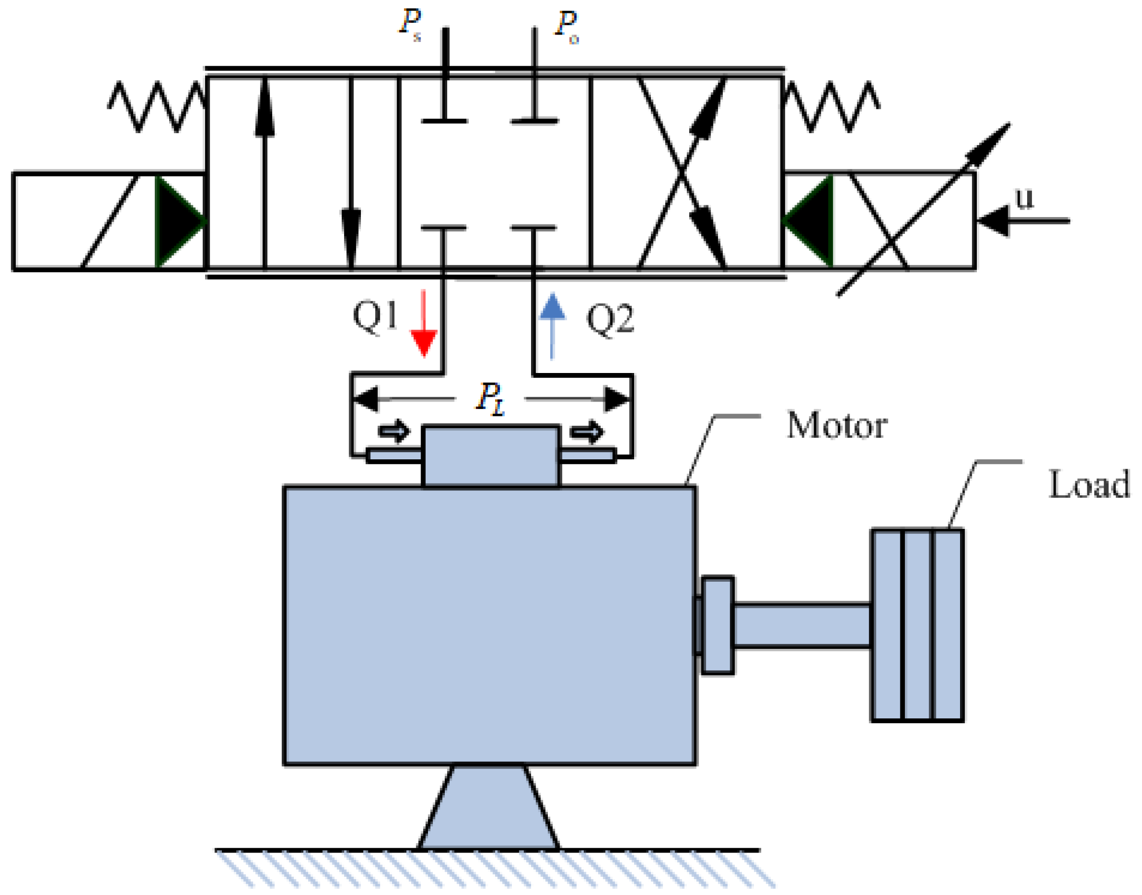
2. Mathematical Model and Problem Description

The system model of the valve-controlled motor is built according to the actual needs. The flow into and out of the motor is controlled by electro-hydraulic servo valves, and the motor can track the given signal. The model is shown in Figure 1.

The structure of the electro-hydraulic position servo system is shown in Figure 1. According to Newton’s second law, the force balance equation of the load can be obtained as:

$$D_m{P}_L=J\ddot{\theta }+B\dot{\theta }+F$$

(1)

where J is the rotational inertia of the motor, $D_m$ is the displacement of the hydraulic motor, $\theta$ is the angle of rotation of the valve motor, $P_L=P_1-P_2$ is the hydraulic motor load pressure, $P_1$ and $P_2$ are the hydraulic motor two cavity pressure, B is the coefficient of viscous friction, and F is the load force.

The hydrodynamic model of the servo valve is nonlinear. There is a mathematical relationship between the output of the load flow and the spool displacement can be expressed as [21]

$$Q_L=C_d\omega x_v\sqrt{\frac{P_S-P_{L}sign\left(x_v\right)}{\rho }}$$

(2)

where $Q_L$ is the output fluid, $C_d$ is the servo valve orifice flow coefficient, $\omega$ is the servo valve throttle area gradient, $x_v$ is the displacement of the servo valve spool, $P_S$ is the pressure of the fluid, and $\rho$ is the density of the fluid.

The continuity equation between the load flow and the hydraulic oscillating motor flow is

$$Q_L=D_m\dot{\theta }+C_t{P}_L+\frac{V}{4{\beta }_e}{\dot{P}}_L-Q\left(t\right)$$

(3)

where $C_t$ is the total leakage coefficient of the hydraulic motor, $V$ is the total volume of the two chambers connected to the main pipe, ${\beta }_e$ is the effective volume elastic modulus, and $Q\left(t\right)$ is the time-varying uncertain flow in the servo system.

The servo valve in this paper operates at a much higher frequency than the hydraulic oscillating motor. To simplify the connection between the motor and the servo valve, the dynamics of the servo valve can be simplified to a proportional relationship [22].

$$x_v=k_i{u}_t$$

(4)

where $k_i$ is dynamic proportional coefficient of the servo valve, $u_t$ is the control voltage.

Then Equation (2) can be expressed as

$$Q_L=K_t{u}_t\sqrt{P_S-P_{L}sign\left(u_t\right)}$$

(5)

where $K_t=C_d\omega k_i\sqrt{1/\rho }$.

To simplify controller design, the system state variable is chosen as: $X={\left[\begin{array}{ccc}{x}_1& x_2& x_3\end{array}\right]}^T$. According to Equations (1)–(5), the state space expression of the electro-hydraulic servo system is

$$\dot{X}=\left[\begin{array}{c}\dot{x_1}\\ \dot{x_2}\\ \dot{x_3}\end{array}\right]=\left[\begin{array}{c}{x}_2\\ f_1(x_3)+f_2(x_2)+d(t)\\ f_3(u_t,x_3)u_t+f_4(x_2,x_3)+q(t)\end{array}\right]$$

(6)

$$y=\left[1 0 0\right]x$$

(7)

where $f_1\left(x_3\right)=\frac{D_m}{J}{x}_3$,$f_2\left(x_2\right)=-\frac{B}{J}{x}_2$, $d\left(t\right)=-\frac{F}{J}$,$f_3\left(u_t,x_3\right)=\frac{4{\beta }_e{K}_t}{V}\sqrt{P_s-x_3\mathrm{sign}\left(u_t\right)}$, $f_4\left(x_2,x_3\right)=-\frac{4{\beta }_e}{V}\left(D_m{x}_2+C_t{x}_3\right)$, $q\left(t\right)=\frac{4{\beta }_{e}Q\left(t\right)}{V}$.

In order to make the derivation and design of the system convenient, the following assumptions are made:

• The pressure in each chamber of the hydraulic rotary motor is equal everywhere.
• The total amount of liquid leakage is negligible that is $Q\left(t\right)$ = 0.
• Ignoring the non-linear interference such as friction and the influence of fluid quality.

3. Sliding Mode Controller Design

The design of the slide controller can be divided into two steps, including the design of the slide surface and the design of the control law.

3.1. Design of Slide Surface

Defining the electro-hydraulic position servo system position tracking error $e$, velocity tracking error $\dot{e}$, acceleration tracking error $\ddot{e}$, acceleration derivative tracking error $\stackrel{⃛}{e}$, ${\theta }_d$ is the given signal, according to the Equations (6) and (7) can be expanded as

$$e=\theta -{\theta }_d=x_1-{\theta }_d$$

(8)

$$\dot{e}=\dot{\theta }-\dot{{\theta }_d}=x_2-\dot{{\theta }_d}$$

(9)

$$\ddot{e}=\ddot{\theta }-\ddot{{\theta }_d}=\frac{1}{J}\left[D_m{x}_3-B{x}_2-F\right]-\ddot{{\theta }_d}$$

(10)

$$\stackrel{⃛}{e}=\stackrel{⃛}{\theta }-\stackrel{⃛}{{\theta }_d}$$

(11)

$$\stackrel{⃛}{e}=\frac{1}{J}\left[\frac{4D_m{\beta }_e{k}_t{u}_t}{V}\sqrt{P_S-x_{3}sign\left(u_t\right)}+\left(B^2-\frac{D_m^2{\beta }_e}{V}\right)x_2-\left(\frac{4D_m{\beta }_e{c}_t}{V}+B{D}_m\right)x_3+\frac{B}{J}F\right]-\stackrel{⃛}{{\theta }_d}$$

(12)

Designing the sliding mode surface of the controller is $s$:

$$s=c_{1}e+c_2\dot{e}+\ddot{e}$$

(13)

where $c_1>0$, $c_2>0$, and the derivative of Equation (13) can be obtained:

$$\dot{s}=c_1\dot{e}+c_2\ddot{e}+\stackrel{⃛}{e}$$

(14)

Simplifying and combining Equations (8)–(14) will obtain:

$$\dot{s}=A_1{x}_2+A_2{x}_3-c_1{\dot{\theta }}_d-c_2{\stackrel{\dot{}\dot{}}{\theta }}_d-{\stackrel{\dot{}\dot{}\dot{}}{\theta }}_d+A_3\sqrt{P_S-x_{3}sign(u_t)}{u}_t+(\frac{B}{J^2}-\frac{c_2}{J})F$$

(15)

where $A_1=\left(c_1-\frac{c_{2}B}{J}-\frac{4{\beta }_e{D}_m{}^2}{JV}+\frac{B^2}{J^2}\right)$, $A_2=\left(\frac{c_2{D}_m}{J}-\frac{4{\beta }_e{D}_m{C}_t}{JV}-\frac{B{D}_m}{J^2}\right)$, $A_3=\frac{4{\beta }_e{D}_m{K}_t}{JV}$.

The exponential convergence law [23] is used as the convergence law for designing the sliding mode controller as:

$$\dot{s}=-\beta s-\eta sign\left(s\right)$$

(16)

where $\beta$ and $\eta$ are the controller discontinuity term gain, and $\beta$> 0, $\eta$> 0.

According to Equations (15) and (16), the controller output $u_t$ can be designed as:

$$u_t=\frac{A_4[-\beta s-\eta sign(s)+c_1{\dot{\theta }}_d+c_2{\stackrel{\dot{}\dot{}}{\theta }}_d+{\stackrel{\dot{}\dot{}\dot{}}{\theta }}_d+(\frac{c_2}{J}-\frac{B}{J^2})F+A_5{x}_2+A_6{x}_3]}{\sqrt{P_S-x_{3}sign(u_t)}}$$

(17)

where $A_4=\frac{JV}{4{\beta }_e{D}_m{K}_t}$,$A_5=\left(-c_1+\frac{c_{2}B}{J}+\frac{4{\beta }_e{D}_m{}^2}{JV}-\frac{B^2}{J^2}\right)$,$A_6=\left(-\frac{c_2{D}_m}{J}+\frac{4{\beta }_e{D}_m{C}_t}{JV}+\frac{B{D}_m}{J^2}\right)$.

Based on this controller, the sliding surface of the system can be made to converge to 0, which is the steady state.

3.2. System Stability Analysis of Sliding Mode Control

According to the stability analysis of the system in control theory, the Lyapunov function is defined as:

$$L=\frac{1}{2}{s}^2$$

(18)

Derivation of Equation (18) and substitution of Equation (15) can be obtained:

$$\dot{L}=s, \dot{s}=s\left(-\beta s-\eta sign\left(s\right)\right)=-\beta s^2-\eta \left|s\right|\le 0$$

(19)

The above equations show that the Lyapunov function L is positive definite and its derivative is negative definite, thus the system will reach a steady state. This means that the sliding mode surface $s$ will be stable in finite time, and thus the system can be proved to be asymptotically stable.

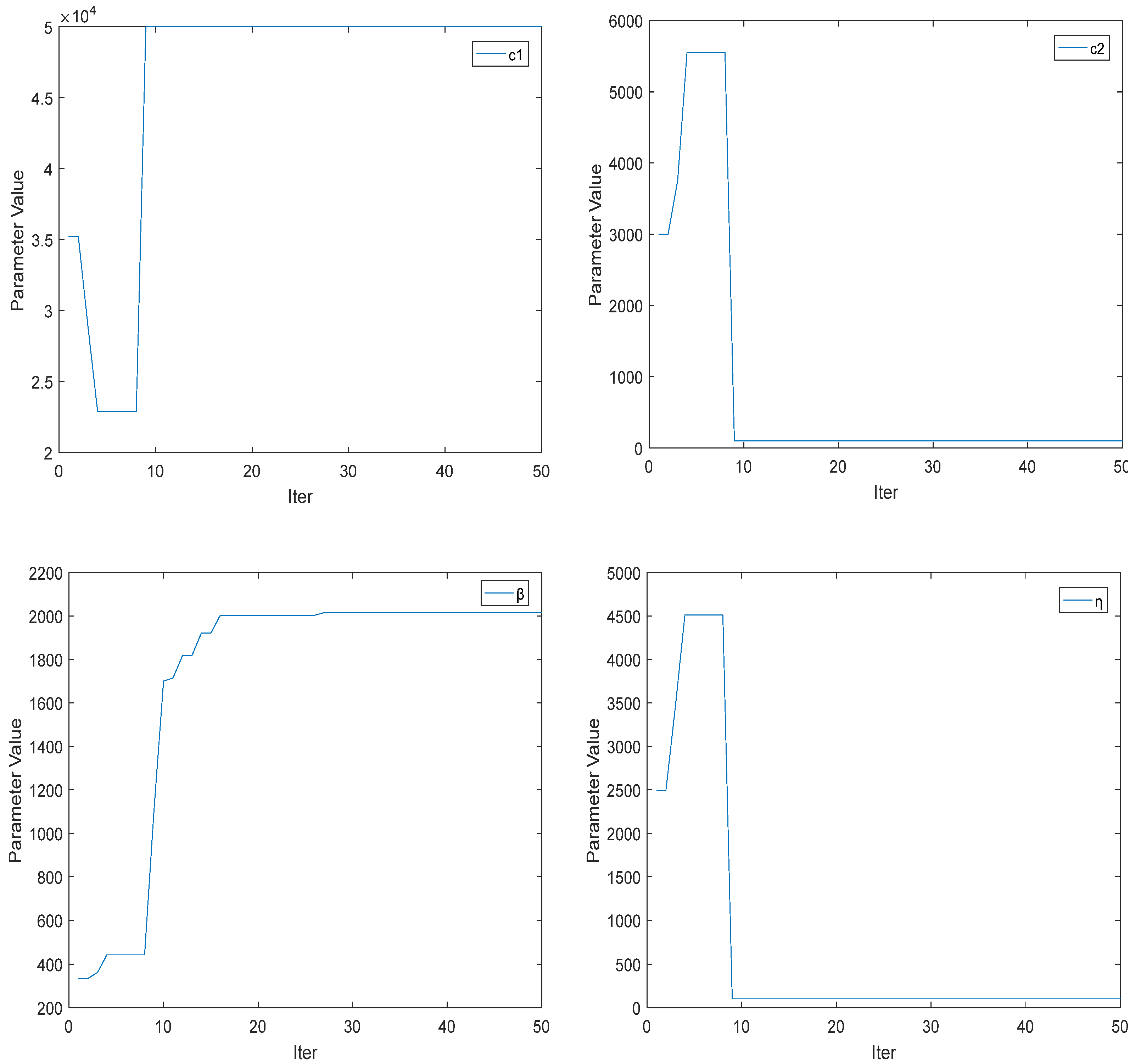
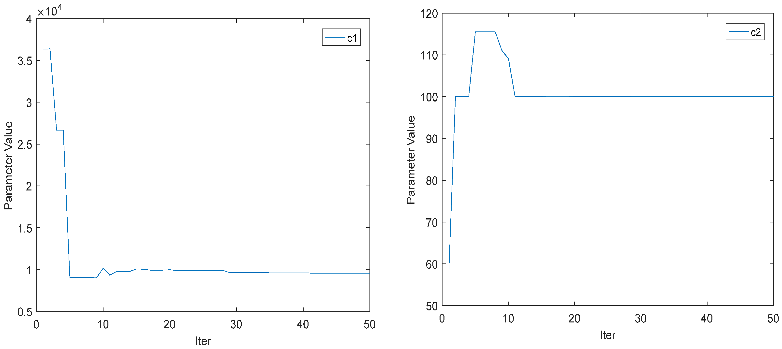
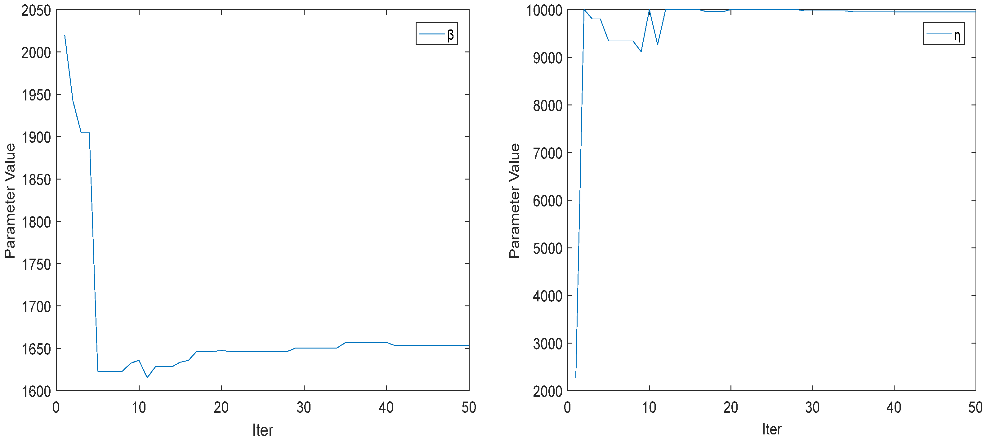
4. Quantum Particle Swarm Algorithm to Optimize Parameters

Although the sliding mode controller has good control performance for electro-hydraulic servo system, if the selected parameters are not suitable it will lead to failure to track, large tracking error, jitter, etc. Therefore, in this paper the optimization algorithm is chosen to optimize the parameters of the controller.

The QPSO algorithm removes the relationship between the update of the particle position and the previous position of the particle. This relationship will lead to a limited search space and trap in a locally optimal solution. Removing these restrictions will increase the particle search space and improve randomness, as the particle can appear at any position in the search interval as far as possible. The adaptation value of this random point will be compared with the current best adaptation value to make a choice, and finally the algorithm gets the global optimal solution through continuous iterations. There is only one parameter to choose in the algorithm which also makes it easier to implement.

The QPSO algorithm has the above effect, so QPSO algorithm is used in this paper to optimize the parameters of the system.

4.1. Evolution Equation of Particle Swarm Algorithm

The PSO algorithm performs a parameter search mainly by updating its own velocity and position. The particle searches for the local optimal solution and continuously updates the global optimal solution to obtain the optimal fitness value in each iteration.

Velocity update formula:

$$ve{l}_n=ve{l}_n+r_1\times rand()\times (pbes{t}_n-x_n)+r_2\times rand()\times (gbes{t}_n-x_n)$$

(20)

Position update formula:

$$x_n=x_n+ve{l}_n$$

(21)

where $ve{l}_n$ is the velocity of the particle, $\mathit{rand}()$ is a random number between (0, 1), $x_n$ is the position of the particle, $\mathit{pbest}$ and $\mathit{gbest}$ are the best position of individual and the best position of the group respectively, and $r_1$ and $r_2$ are the learning coefficient; usually taking two can obtain better results.

4.2. Flow of Quantum Particle Swarm Algorithm

Supposing a particle swarm containing M particles is searched in an N-dimensional target space, and M potential problems form the population:

$$X\left(t\right)=[X_1\left(t\right), X_2\left(t\right), \dots X_M\left(t\right)]$$

(22)

Then the position of the i-th particle is $X_i\left(t\right)=\left[X_{i,1}\left(t\right),X_{i,2}\left(t\right),\cdots ,X_{i,N}\left(t\right)\right],i=1,2,\cdots M$ at time t.

Using $P_i\left(t\right)=\left[P_{i,1}\left(t\right),P_{i,2}\left(t\right),\cdots ,P_{i,N}\left(t\right)\right]$ to indicate the best position of individual, $G_i\left(t\right)=\left[G_{i,1}\left(t\right),G_{i,2}\left(t\right),\cdots ,G_{i,N}\left(t\right)\right]$ indicates the best position of the group.

The individual best position of particle i depends on the objective function. The individual best position of particle i:

$$P_i\left(t\right)=\{\begin{array}{c}{X}_i\left(t\right) if f\left[X_i\left(t\right)\right]<f\left[P_i\left(t-1\right)\right]\\ P_i\left(t-1\right) if f\left[X_i\left(t\right)\left]\ge f\right[P_i\left(t-1\right)\right]\end{array}$$

(23)

The global best position of the population is determined by Equations (22) and (23):

$$g=\arg \underset{1\le i\le M}{\min }\left\{f\left[P_i\left(t\right)\right]\right\}$$

(24)

$$G\left(t\right)=P_g\left(t\right)$$

(25)

Evolutionary equations for the quantum particle swarm algorithm:

$$X_j\left(t+1\right)=P_j\left(t\right)+\alpha \left|C_j\left(t\right)-X_j\left(t\right)\right|\ln \frac{1}{u}$$

(26)

$$P_{i,j}=g{P}_{i,j}+\left(1-g\right)G_j$$

(27)

$$C_j\left(t\right)=\frac{1}{M}{\displaystyle \sum }_{i=1}^M{P}_{i,j}\left(t\right)$$

(28)

where $g$ and u are random numbers within [0,1], which are used to represent the average distribution law.

From Equations (26)–(28), we can get a randomness in the position update of the QPSO algorithm, which can make the particles perform global search in the whole search range. Compared with the evolutionary equations of PSO algorithm, QPSO algorithm can perform a better global search to avoid getting trapped in local optimal solutions.

The steps of the quantum particle swarm algorithm are as follows:

• Setting the initial data, including population size, maximum number of iterations, dimension, parameter search range, range of scaling factors, etc.
• Calculating the average best position of the particle population according to Equation (28).
• Performing steps 4–7 for each particle.
• Calculating the adaptation value of the current position of particle i and update the individual best position of the particle according to Equation (23).
• Comparing the individual best position of particle i $P_i\left(t\right)$ with the adaptation value of the global best position G(t−1). If $f\left[P_i\left(t\right)\right]<f\left[G\left(t-1\right)\right]$, it is set $G\left(t\right)=P_i\left(t\right)$, otherwise $G\left(t\right)=G\left(t-1\right)$.
• Calculating the position of a random point according to Equation (27) for each dimension of particle i.
• Updating the new position of the particle according to Equation (26).

The only parameter that needs to be set during the search of the quantum particle swarm algorithm is the contraction-expansion factor in Equation (26), which is taken as

$$\alpha ={\alpha }_{\min }+({\alpha }_{\max }-{\alpha }_{\min })\frac{i_{\max }-i}{i_{\max }}$$

(29)

where ${\alpha }_{\max }=1,{\alpha }_{\min }=0$.

The shrink-expansion coefficient $\alpha$ can affects the speed of search. At the beginning of the algorithm, a faster searching speed is needed to approach the global optimum, so a larger value of $\alpha$ is needed at this time. After the algorithm obtains the global optimum, it is necessary to strengthen the local search ability so that it can further improve the effect of the parameters, so the searching speed can be reduced at this time. In choosing the method of linear decrease of Equation (29) to search, the value of $\alpha$ from large to small is suitable for the search of the algorithm.

The QPSO algorithm performs a global search in the initial stage and local search in the later stage under the influence of the contraction-expansion factor. This ensures that the algorithm has the advantage of searching both the global and local search.

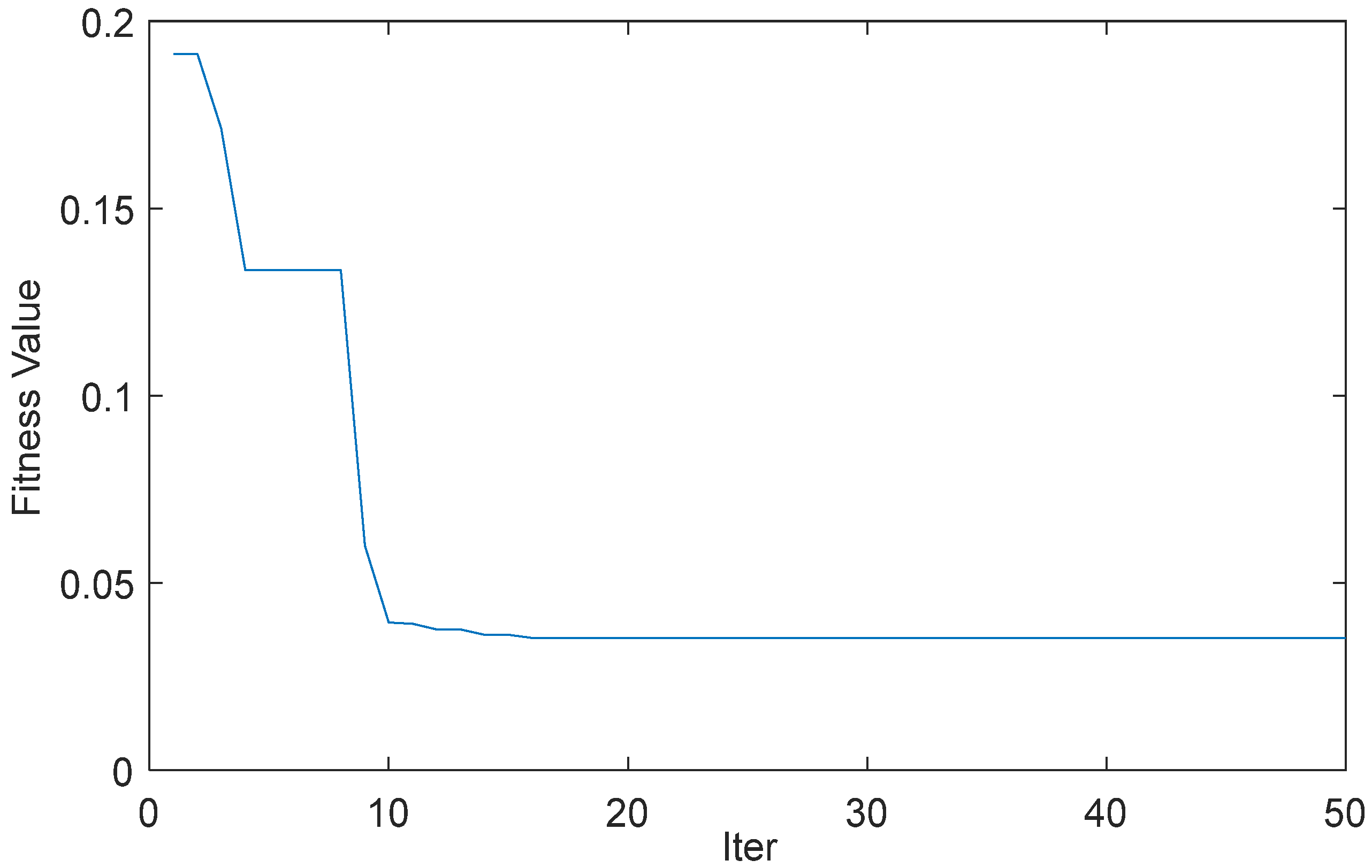
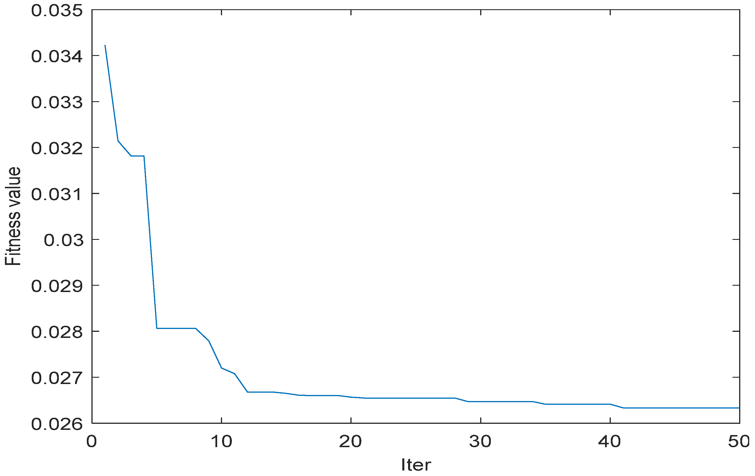
4.3. Fitness Function

The fitness function is an important indicator for the algorithm to evaluate the superiority of the parameters, so a suitable function should be selected for evaluation. The fitness function chosen in this paper is the ITAE indicator:

The fitness function Z chosen in this paper is the ITAE indicator:

$$Z={\displaystyle \int }t\left|e\left(t\right)dt\right|$$

(30)

where $e\left(t\right)$ is the tracking error of the system.

This indicator can reflects the overall error accumulation of the system in operation, and effectively screens out parameters in the experiment. The cumulative error in the whole period of time and the error of each time are significantly reduced when fitness value is smaller, so the system can get better tracking performance. The index is effective in considering the system stability and performance, it is a kind of control system performance evaluation index with good engineering practicality and selectivity. The transient response oscillations of the system evaluated by this index will be reduced, and the indicator has good selectivity for parameters.

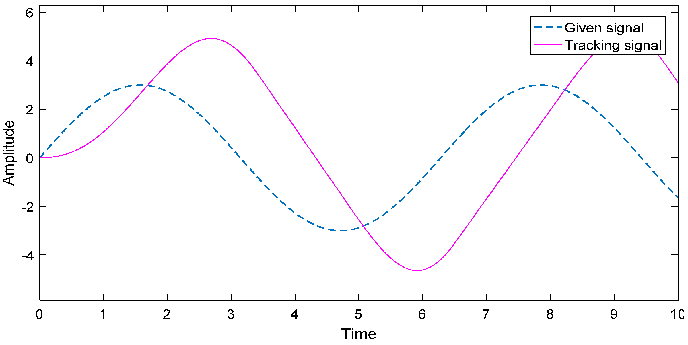
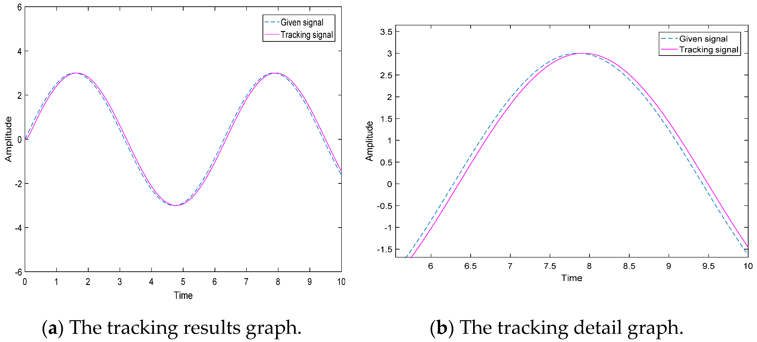
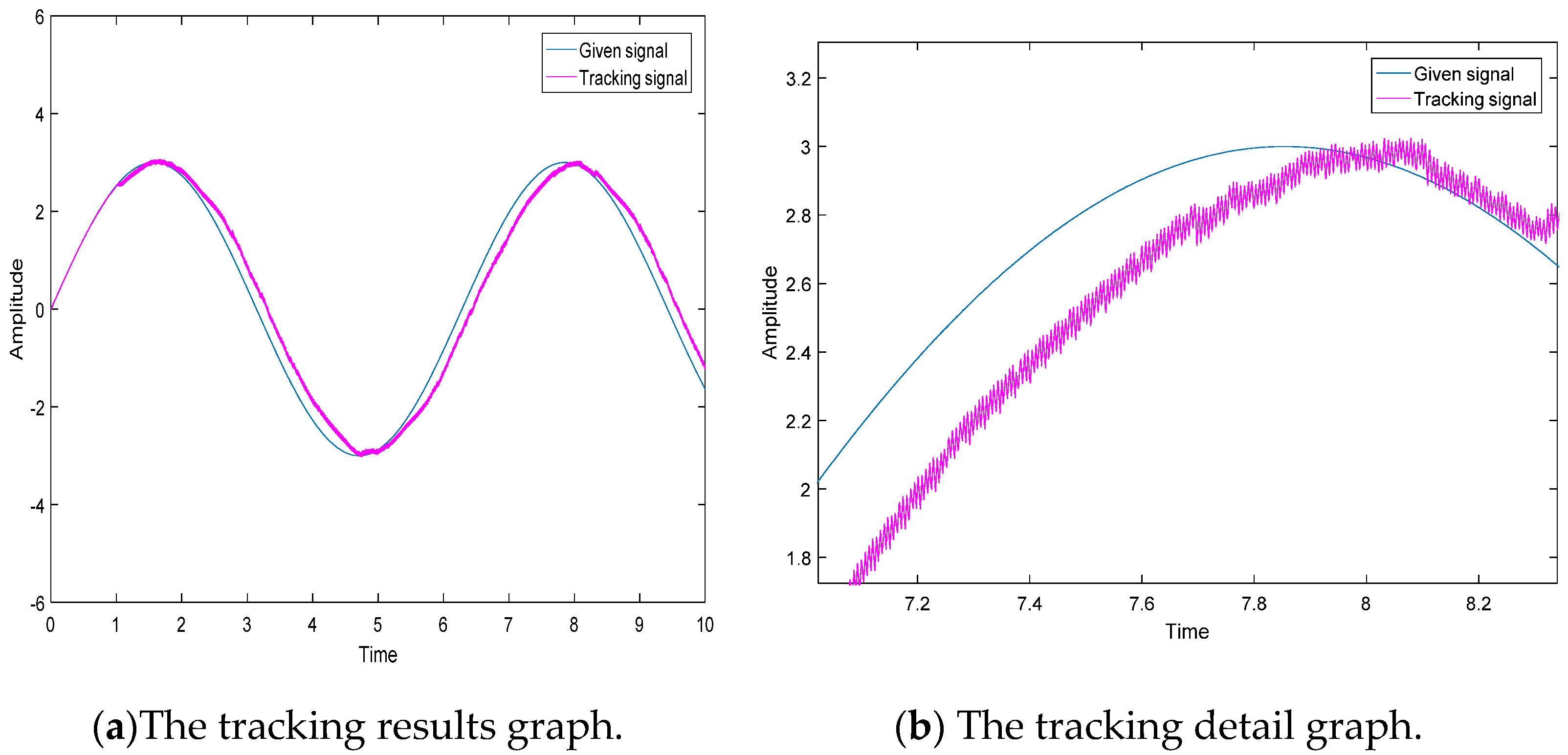
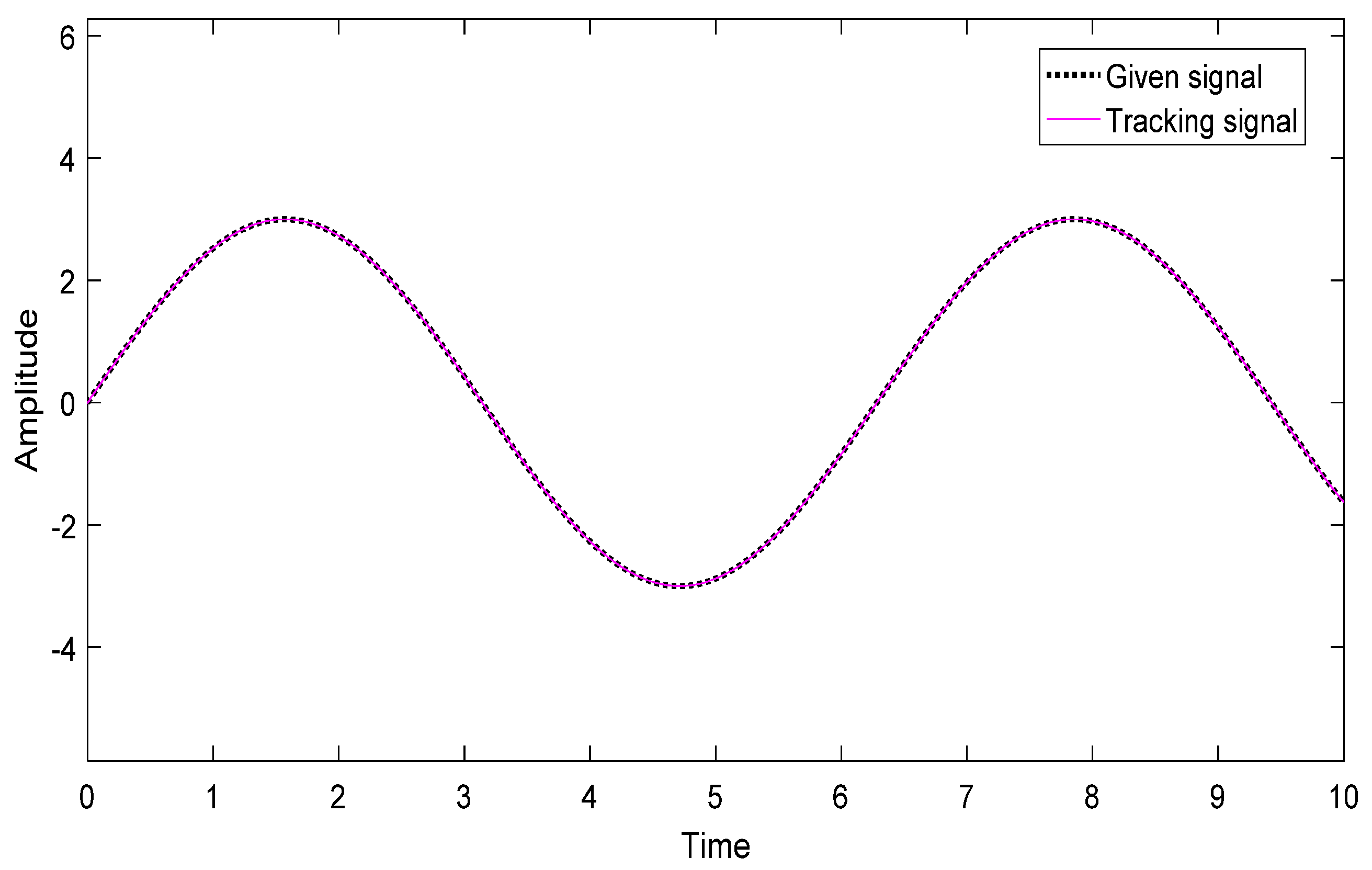
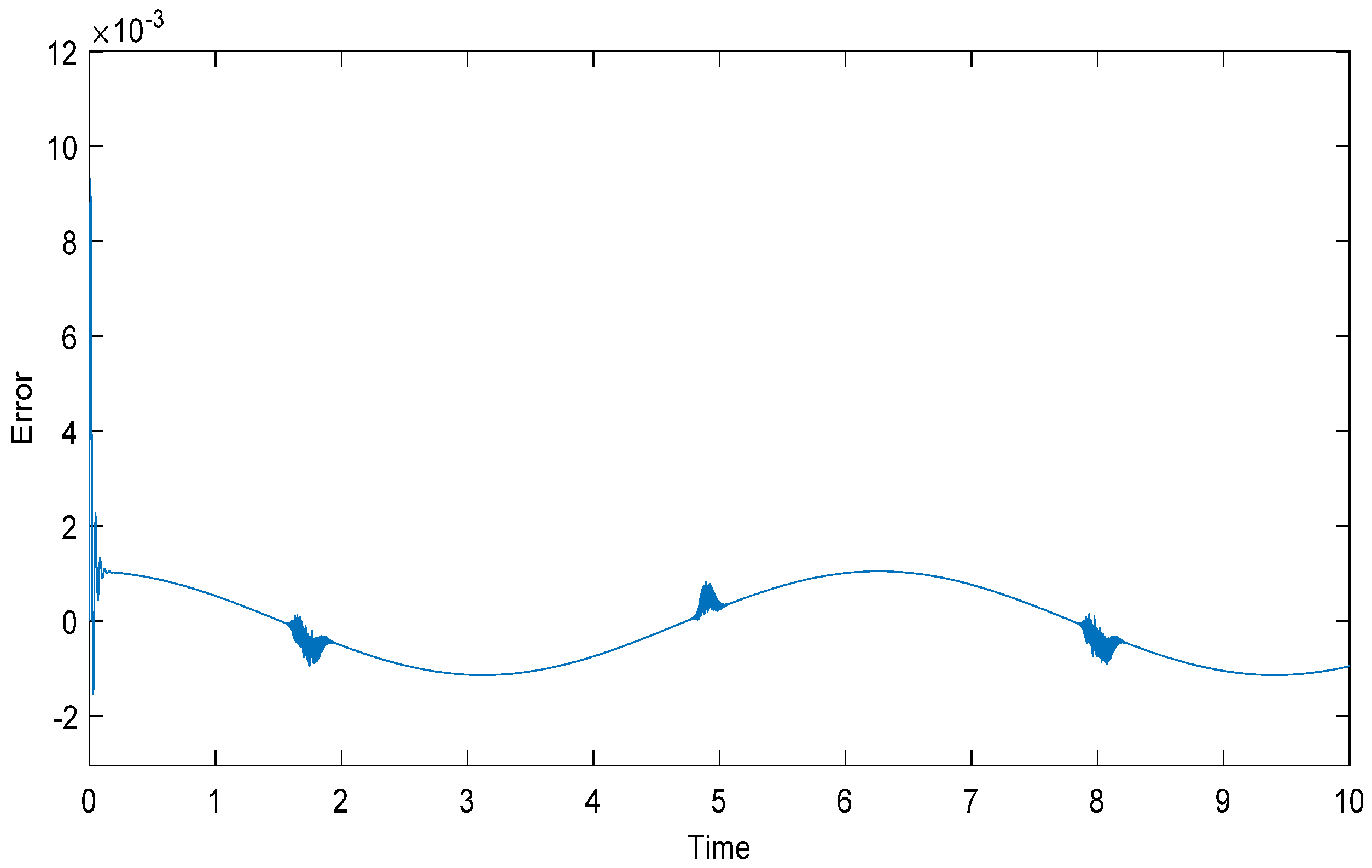
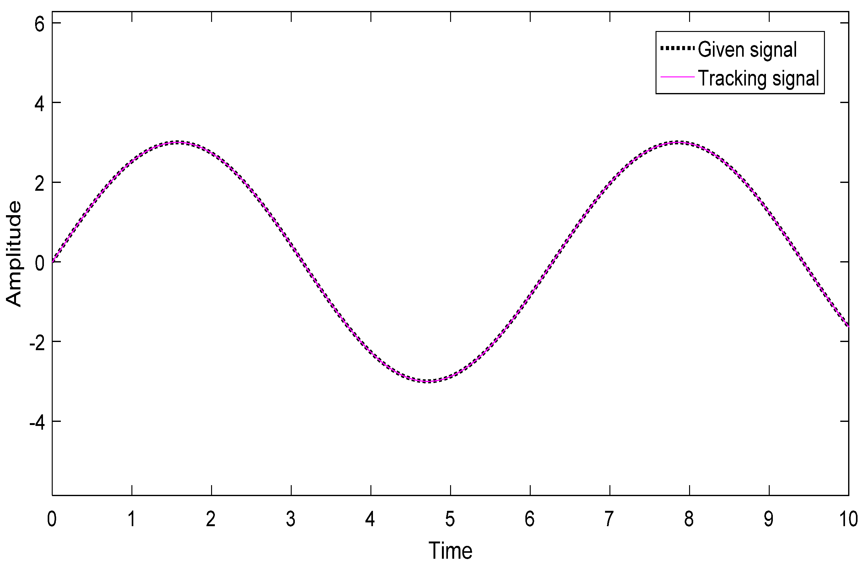
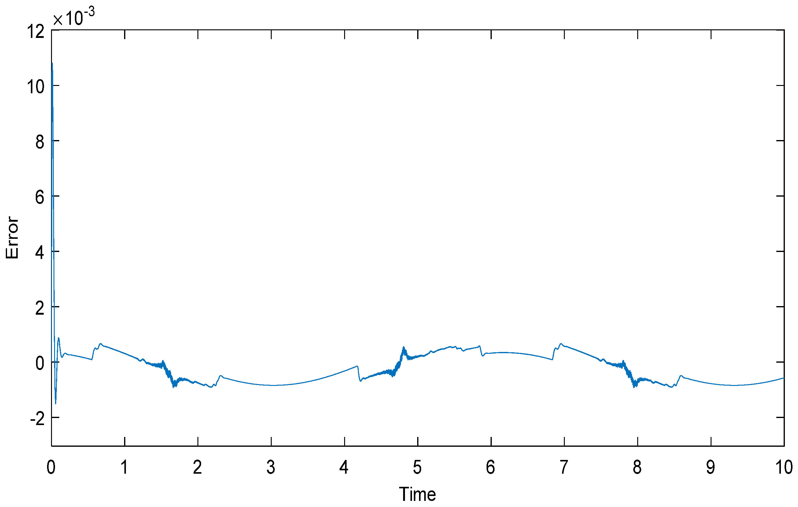
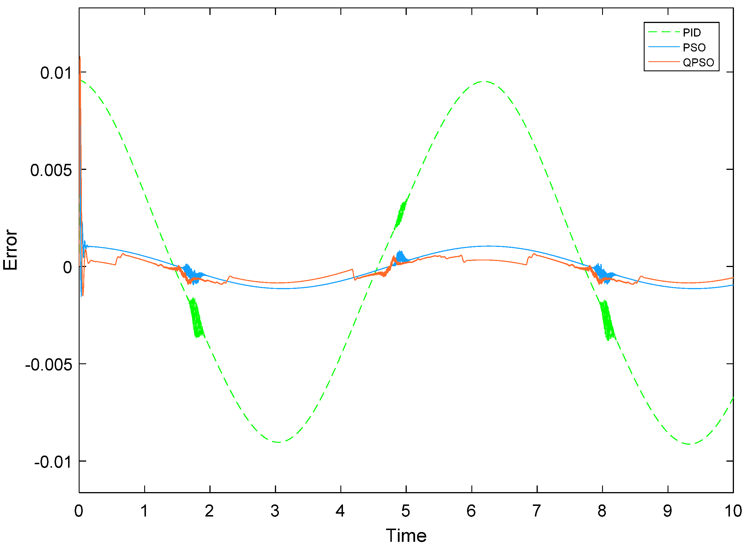
5. Simulation Analysis

To verify the proposed control strategy, the system simulation model is built in Matlab/Simulink, the simulation step is set to 0.001 s, and the load force F is set to 10 N. Due to the actual engineering of the electro-hydraulic servo system structures are easy to damage when subjected to excessive voltage and current, control torque, so the output of controller in the simulation is limited to between $\left(-10,+10\right)$. The data for the electro-hydraulic servo system parameters are shown in

Table 1. System Parameters.

System Parameters	Value
Dm	$8.7\times {10}^{-5}{ \mathrm{m}}^3/\mathrm{rad}$
J	$0.25 \mathrm{kg}·{\mathrm{m}}^2$
B	$40 (\mathrm{N}·\mathrm{m}·\mathrm{s})/\mathrm{rad}$
Vt	$1.4\times {10}^{-4}{ \mathrm{m}}^3$
Kt	$2.16\times {10}^{-8}{ \mathrm{m}}^3/\left(\mathrm{s}·\mathrm{V}·{\mathrm{Pa}}^{1/2}\right)$
βe	$7\times {10}^8 \mathrm{Pa}$
Ct	$1\times {10}^{-2} \left({\mathrm{m}}^3/\mathrm{s}\right)/\mathrm{Pa}$

.

The parameters of the hydraulic system are as follows:

In order to verify the effectiveness of the design for the electro-hydraulic servo system, three working conditions are investigated for comparative simulation experiments. Selecting the given signal as ${\theta }_d=sin\left(t\right)$, the amplitude is $\pm 3$ rad/s.

5.1. Working Condition I

Selecting the controller parameters as $c_1$ = 100, $c_2$ = 10, $\beta$ = 10, $\eta$ = 10.

Figure 2 shows the inability to track a given signal when the parameters are not properly selected, the error between the amplitude of the output curve, and the given signal is large. The sliding mode controller is unable to control the system, and the maximum error reaches 3.62 rad/s.

Selecting the controller parameters as $c_1$ = 15,000, $c_2$ = 10, $\beta$ = 10, $\eta$ = 10.

From Figure 3, it can be observed that the tracking accuracy may not be accurate enough when the parameters are not selected properly, and the phase of the tracking curve lags behind the given curve. The tracking error is between ±0.21 rad/s, which is poor tracking for systems that require high precision control.

Selecting the controller parameters as $c_1$ = 13,000, $c_2$ = 400, $\beta$ = 2600, $\eta$ = 20,000.

From Figure 4, it can be obtained that the jitter may occur when the parameters are not selected properly. The output curve has obvious jitter phenomenon, which may make the system unstable and lead to damage of the machine. The tracking error is between ±0.128 rad/s, and the curve has a jitter amplitude of 0.1 rad/s.

From the above situation, it can be deduced that the sliding mode controller may produce several situations before the parameters are properly selected: it cannot track the upper signal, the tracking error is large, and the tracking curve and the jitter of the controller output are problems. It shows that the selection of parameters has a large impact on the control performance.

5.2. Working Condition II

It can be seen from Working condition I that the control effect of the sliding mode controller without parameter optimization is not satisfactory. Thus, the PSO algorithm is added to optimize the parameters of the sliding mode controller in this case.

Taking a population size of 20, a maximum number of iterations of 50, and a dimension of 4, the upper and lower limits of $\left[c_1,c_2,\beta ,\eta \right]$ are taken as $\left[50,000, 10,000, 20,000, 10,000\right]$ and $\left[100,100,100,100\right]$.

From Figure 5, it can be obtained that the controller parameters take the values $c_1$ = 50,000, $c_2$ = 100, $\beta$ = 1827.8, $\eta$ = 100 after the optimization of the PSO algorithm. It can be seen that the parameters fall into the local optimal solution after the tenth iteration and it is difficult to jump out of the local optimal solution resulting in the optimal parameters not being updated.

From Figure 6, it can be seen that the fitness value curve gradually falls into the local optimal solution after the 10th iteration. The optimal fitness value is not effectively reduced due to the fact that the subsequent local search capability is not strong, which is detrimental to the search for parameters.

From Figure 6, Figure 7 and Figure 8, it can be found that the sliding mode controller can track the given signal after optimizing the parameters by PSO algorithm. The problems of not being able to track the upper signal, large tracking error, tracking curve, and jitter of the controller output that appear in working condition I have been greatly improved. However, there are still problems in the details of optimization. After the 10th iteration of the PSO algorithm, the algorithm falls into a local optimum solution and the fitness value hardly improves. This problem indicates that the particle finds a locally optimal solution and then starts a region search near that solution, thus the particle misses other better solutions.

5.3. Working Condition III

From Case 2, it can be seen that the sliding mode controller can better achieve the position tracking of the given signal after the optimization of the parameters by the PSO algorithm. However, the PSO algorithm is easy to fall into the local optimal solution control and the control accuracy needs to be further improved, so the QPSO algorithm is used to optimize the parameters of the sliding mode controller in Case 3.

Taking a population size of 20, a maximum number of iterations of 50, and a dimension of 4, the upper and lower limits of $\left[c_1,c_2,\beta ,\eta \right]$ are taken as $\left[50,000, 10,000, 20,000, 10,000\right]$ and $\left[100,100,100,100\right]$.

From Figure 9, it can be obtained that the controller parameters take the values of $c_1$ = 9590.215, $c_2$ = 100.04, $\beta$ = 1653.069, $\eta$ = 9950.2 after the optimization of the QPSO algorithm. It can be seen that after the global search in the first stage, the QPSO algorithm has better performance in the later stages of the search.

The algorithm continuously performs a global search and updates the global optimal solution several times in the first stage of the search, while the QPSO algorithm finds the parameters that better fit the system near the optimal solution at a later stage of the algorithm. Comparing with Figure 6, the optimal adaptation degree is improved by 25%, which illustrates that the PSO algorithm falls into the local optimal solution.

From Figure 10, Figure 11 and Figure 12,compared with the traditional sliding mode control, the complex operation of manually adjusting the system parameters can be omitted and the jitter problem of the system and controller output can be effectively eliminated. Compared with the parameters optimized by the particle swarm algorithm, the QPSO algorithm can go beyond the local optimal solution to obtain the global optimal solution, and the optimized parameters can achieve better performance of the system.

Because the electro-hydraulic servo system is a high-precision system, the evaluation function selected in this paper is the ITAE metric, so the selection for the parameters is based on the magnitude of the error and the accumulated value of the error. The final results show that the accuracy of the system has been greatly improved and the jitter of the system based on the QPSO algorithm still exists, but it has been improved compared to the jitter in Figure 4.

In Figure 13, the tracking error after the system is controlled by the PID controller is added for comparison. The values of the PID controller parameters are $\mathrm{P}=800, \mathrm{I}=100, \mathrm{D}=0$.

From Figure 13 and

Table 2. Data Analysis.

Fitness Value	Average Value	Standard Deviation	Optimum Value
PSO algorithm	0.0548	0.0445	0.0353
QPSO algorithm	0.0271	0.0017	0.0263

, it can be concluded that the error range of the system after being controlled by the PID controller is $-9.5\times {10}^{-3}~9.5\times {10}^{-3}$, and the tracking error range of the system after the optimization of the PSO algorithm is $-1.14\times {10}^{-3}~1.05\times {10}^{-3}$. The tracking error range of the system after optimization by the QPSO algorithm is $-9.22\times {10}^{-4}~6.63\times {10}^{-4}$ and the margin of error is reduced $36.8\%$ compared to PSO algorithm. The fitness value reduced by $25\%$ reflects a reduction in the overall error accumulation, a more stable system, a faster rate of reaching stability, and a significant increase in tracking accuracy.

According to the above three working conditions, it can be observed that compared with the traditional sliding mode control and PSO algorithm optimized sliding mode control, the sliding mode controller optimized by QPSO algorithm has a greater improvement in all aspects of control performance, which reflects that the method has a better control effect for the system under the operation with load force.

6. Conclusions

In this paper, the sliding mode controller based on QPSO algorithm for parameter optimization was proposed to address the nonlinear problem of electro-hydraulic servo systems, external disturbance, and the problem of controller parameter selection. The sliding mode controller with strong robustness can track a given signal, and then QPSO algorithm based on ITAE metric is used to optimize the parameters of the sliding mode controller. This design expands the search space of parameters, diminishes the effect of jitter, and achieves the global optimal solution; thus, the control performance of electro-hydraulic servo system is improved. The experiments show that compared with the PSO algorithm, the fitness value is reduced by 25% and the tracking accuracy of the system is improved by 36.8% after optimization by QPSO algorithm. The algorithm not only eliminates the complexity of manually adjusting parameters but also effectively performs a global search; finally the electro-hydraulic servo system achieves improved tracking performance under load forces.

References

1. Huang, Y.; Pool, D.M.; Stroosma, O.; Chu, Q. Long-stroke hydraulic robot motion control with incremental nonlinear dynamic inversion. IEEE/ASME Trans. Mechatron. 2019, 24, 304–314. [Google Scholar]
2. Sun, W.; Pan, H.; Gao, H. Filter-based adaptive vibration control for active vehicle suspensions with electrohydraulic actuators. IEEE Trans. Veh. Technol. 2015, 65, 4619–4626. [Google Scholar]
3. Iwasaki, M.; Seki, K.; Maeda, Y. High-precision motion control techniques: A promising approach to improving motion performance. IEEE Ind. Electron. Mag. 2012, 6, 32–40. [Google Scholar]
4. Tang, W.; Xu, G.; Zhang, S.; Jin, S.; Wang, R. Digital Twin-Driven Mating Performance Analysis for Precision Spool Valve. Machines 2021, 9, 157. [Google Scholar]
5. Nguyen, M.H.; Dao, H.V.; Ahn, K.K. Active Disturbance Rejection Control for Position Tracking of Electro-Hydraulic Servo Systems under Modeling Uncertainty and External Load. Actuators 2021, 10, 20. [Google Scholar]
6. Feng, H.; Ma, W.; Yin, C.; Cao, D. Trajectory control of electro-hydraulic position servo system using improved PSO-PID controller. Autom. Constr. 2021, 127, 103722. [Google Scholar]
7. Yu, L.-K.; Zheng, J.-M.; Yuan, Q.-L.; Xiao, J.-M.; Li, Y. Fuzzy PID control for direct drive electro-hydraulic position servo system. In Proceedings of the 2011 International conference on consumer electronics, communications and networks (CECNet), Xianning, China, 16–18 April 2011; IEEE: Piscataway, NJ, USA, 2011; pp. 370–373. [Google Scholar]
8. Milić, V.; Šitum, Ž.; Essert, M. Robust H∞ position control synthesis of an electro-hydraulic servo system. ISA Trans. 2010, 49, 535–542. [Google Scholar]
9. Aela, A.; Mohamed, A.; Kenne, J.P.; Angue Mintsa, H. A novel adaptive and nonlinear electrohydraulic active suspension control system with zero dynamic tire liftoff. Machines 2020, 8, 38. [Google Scholar]
10. Feng, L.; Yan, H. Nonlinear adaptive robust control of the electro-hydraulic servo system. Appl. Sci. 2020, 10, 4494. [Google Scholar]
11. Yue, X.; Yao, J.-Y. Adaptive Integral Robust Control of Electro-hydraulic Load Simulator. Chin. Hydraul. Pneum. 2016, 12, 25. [Google Scholar]
12. Yao, J.; Deng, W. Active disturbance rejection adaptive control of hydraulic servo systems. IEEE Trans. Ind. Electron. 2017, 64, 8023–8032. [Google Scholar]
13. Liu, X.; Huang, R.-N.; Gao, Y.-J. Adaptive Inversion Sliding Mode Control for Electro-hydraulic Servo Motion System. Chin. Hydraul. Pneum. 2019, 7, 14. [Google Scholar]
14. Li, W.-D.; Shi, G.-L. RBF Neural Network Sliding Mode Control for Electro Hydraulic Servo System. Chin. Hydraul. Pneum. 2019, 2, 109. [Google Scholar]
15. Ghazali, R.; Sam, Y.M.; Rahmat, M.F.; Hashim, A. Position tracking control of an electro-hydraulic servo system using sliding mode control. In Proceedings of the 2010 IEEE Student Conference on Research and Development (SCOReD), Kuala Lumpur, Malaysia, 13–14 December 2010; IEEE: Piscataway, NJ, USA, 2010; pp. 240–245. [Google Scholar]
16. Cerman, O.; Hušek, P. Adaptive fuzzy sliding mode control for electro-hydraulic servo mechanism. Expert Syst. Appl. 2012, 39, 10269–10277. [Google Scholar]
17. Liu, L.; Yao, J.Y.; Hu, J.; Ma, D.; Deng, W. Tracking Control for Electro-hydraulic Positioning Servo System Based on Disturbance Observer. Acta Armamentarii 2015, 11, 2053–2061. [Google Scholar]
18. Ming, S. Sliding Mode Control Parameters Tuning Based on Particle Swarm Optimization. Mech. Eng. Autom. 2019, 1, 173–175. [Google Scholar]
19. Cai, G.; Liu, X.; Luo, X.; Chen, H. Sliding Mode Control of Electro-hydraulic Position Servo System Optimized by Improved PSO Algorithm. Mech. Sci. Technol. Aerosp. Eng. 2019, 8, 1223–1230. [Google Scholar]
20. Sun, J.; Lai, C.; Wu, X. Particle Swarm Optimisation: Classical and Quantum Perspectives; Taylor and Francis: Milton Park, UK, 2012; pp. 3–9. [Google Scholar]
21. Shen, W.; Huang, H.; Wang, J. Robust backstepping sliding mode controller investigation for a port plate position servo system based on an extended states observer. Asian J. Control 2019, 21, 302–311. [Google Scholar]
22. Shen, W.; Shen, C. An extended state observer-based control design for electro-hydraulic position servomechanism. Control Eng. Pract. 2021, 109, 104730. [Google Scholar]
23. Jin, B.; Xiong, S.; Cheng, H. Chattering inhibition of variable rate reaching law sliding mode control for electro-hydraulic position servo system. Chin. J. Mech. Eng. 2013, 49, 163–169. [Google Scholar]
Figure 1. The electro-hydraulic servo system model.
Machines 09 00283 g001
Figure 2. Untraceable graph.
Machines 09 00283 g002
Figure 3. Low tracking accuracy graph.
Machines 09 00283 g003
Figure 4. Obvious jitter graph.
Machines 09 00283 g004
Figure 5. The parameter iteration diagram.
Machines 09 00283 g005
Figure 6. The iterative graph of fitness values.
Machines 09 00283 g006
Figure 7. The tracking results graph.
Machines 09 00283 g007
Figure 8. The tracking error value graph.
Machines 09 00283 g008
Figure 9. The parameter iteration diagram.
Machines 09 00283 g009aMachines 09 00283 g009b
Figure 10. The iterative graph of fitness values.
Machines 09 00283 g010
Figure 11. The tracking results graph.
Machines 09 00283 g011
Figure 12. The tracking error value graph.
Machines 09 00283 g012
Figure 13. The tracking error value graph.
Machines 09 00283 g013